HAL Id: hal-02399534
https://hal.archives-ouvertes.fr/hal-02399534
Submitted on 6 May 2021
HAL is a multi-disciplinary open access
archive for the deposit and dissemination of
sci-entific research documents, whether they are
pub-lished or not. The documents may come from
teaching and research institutions in France or
abroad, or from public or private research centers.
L’archive ouverte pluridisciplinaire HAL, est
destinée au dépôt et à la diffusion de documents
scientifiques de niveau recherche, publiés ou non,
émanant des établissements d’enseignement et de
recherche français ou étrangers, des laboratoires
publics ou privés.
Investigating the Role of the Relative Humidity in the
Co-Occurrence of Temperature and Heat Stress
Extremes in CMIP5 Projections
Audrey Brouillet, Sylvie Joussaume
To cite this version:
Audrey Brouillet, Sylvie Joussaume. Investigating the Role of the Relative Humidity in the
Co-Occurrence of Temperature and Heat Stress Extremes in CMIP5 Projections. Geophysical Research
Letters, American Geophysical Union, 2019, 46 (20), pp.11435-11443. �10.1029/2019GL084156�.
�hal-02399534�
Extremes in CMIP5 Projections
Audrey Brouillet1 and Sylvie Joussaume11Laboratoire des Sciences du Climat et de l'Environnement (LSCE-IPSL), CEA/CNRS/UVSQ, Gif-sur-Yvette, France
Abstract
Heat stress is expected to intensify, since temperatures are projected to increase during the 21st century. We investigate the assumed co-occurrence of annual extremes of temperature and one heat stress metric and assess the effect of relative humidity variations on the heat stress changes. We show in CMIP5 simulations that both extremes tend to co-occur in Europe and northern America, when the conditions are the hottest and the driest. However, extreme seasons occur later for heat stress than temperature by up to 2 months within the tropics. By 2100, models project a drying that hampers the increase in heat stress extremes. Within northeastern Africa, the slight projected wettening enhances the warming effect on the heat stress changes and induces the maximum heat stress intensification. Models are generally able to represent the phasing of both extremes compared to observations, with large uncertainties over regions experiencing the greatest future heat stress intensification.Plain Language Summary
Temperature and heat stress extremes are projected to intensify in the future. However, the occurrence and the changes in heat stress extremes also depend on humidity variations. We show that both extremes tend to co-occur during the year in mid-latitudes, but extremes of heat stress tend to occur later than temperature extremes in the tropics, when the relative humidity is annually higher. We also show in future climate simulations that the global projected drying that strengthens the increase in temperature extremes weakens the intensification of heat stress extremes. Nevertheless, this does not prevent risk for health, particularly in tropical areas.1. Introduction
Global mean temperatures are very likely to continue rising during the 21st century (Collins et al., 2013). As global climate is expected to warm in the future, the ensuing heat stress, the well-established combined effect of temperature and humidity on human health, is projected to increase. This heat stress is projected to intensify health risks for population and to decrease labor capacity, particularly over tropical and subtropical areas (Dunne et al., 2013; Zhao et al., 2015). Moreover, the preferential warming of the hot tail of temperature distributions tends to increase the magnitude, frequency, and duration of extremes (Alexander et al., 2006; Meehl, 2004). In previous studies, it was shown that the greatest increase of temperature extremes over land is due to the largest associated drying in midcontinental areas such as Europe, northern America, and Amazonia (Donat et al., 2018; Fischer & Schar, 2010). However, the near-surface relative humidity (RH) and its annual and interannual variations are often overlooked when studying the evolution of the heat stress (Diffenbaugh et al., 2007; Fischer & Knutti, 2013). Yet the impacts of hot extremes on physiology and health can be exacerbated by elevated ambient humidity (Chen et al., 2018; Mora et al., 2017), and a stronger interest in the contribution of the projected changes in humidity is needed.
In this paper, we investigate the potential co-occurrence of extremes of temperature and extremes of the simplified Wet-Bulb Globe Temperature, a commonly used heat stress indicator (Australian Bureau of Mete-orology, 2010; Yaglou & Minard, 1957). We compare their projected changes during the 21st century in order to assess how they are spatially and temporally related. We also analyze the effect of RH variations on the heat stress changes and assess whether the changes in humidity enhance or hamper the global warming effect on the changes in heat stress extremes.
Key Points:
• Temperature and heat stress extremes tend to co-occur in mid-latitudes but are time-lagged in the tropics due to relative humidity • The projected drying (wettening)
weakens (strengthens) the heat stress intensification in midcontinental regions (northeastern Africa) • Despite this weakening effect, future
heat stress is projected to reach the most dangerous health thresholds in the tropics Supporting Information: • Supporting Infomation SI Correspondence to: A. Brouillet, audrey.brouillet@lsce.ipsl.fr Citation:
Brouillet, A., & Joussaume, S. (2019). Investigating the role of the relative humidity in the co-occurrence of temperature and heat stress extremes in CMIP5 projections. Geophysical
Research Letters, 46,
https://doi.org/10.1029/2019GL084156
Received 18 JUN 2019 Accepted 16 SEP 2019
Accepted article online 15 OCT 2019
©2019. The Authors.
This is an open access article under the terms of the Creative Commons Attribution-NonCommercial-NoDerivs License, which permits use and distribution in any medium, provided the original work is properly cited, the use is non-commercial and no modifications or adaptations are made.
11,435–11,443.
Geophysical Research Letters
10.1029/2019GL084156
2. Data and Methods
2.1. Simulated and Observed Data
We analyze data of near-surface air temperature (T), RH, and associated simplified Wet-Bulb Globe Temperature (W) from 1979 to 2100. W is calculated using the simplified equation:
W =0.567 × T + 0.393 × VP + 3.94
with W in no unit or units of W, T the near-surface air temperature (in◦C), and VP the air vapor pressure (in hPa). VP and RH are calculated from daily data of specific humidity (q), sea-level pressure (slp), and T (see Methods in the Supporting Information). Twenty CMIP5 (Taylor et al., 2012) general circulation models (GCMs) provide daily q, slp, and T between 1979 and 2100. We selected one GCM per modelling group among these 20 models and retained 12 GCMs for our multimodel analysis (Table S1). Some models provide several realizations. For these models, each realization is weighted by the total number of realizations available for the model, in order to equally represent all GCMs in multimodel mean values (Chavaillaz et al., 2016). We chose the RCP8.5 scenario since it provides clearer signals as a response to the largest projected warming. We also compare simulations over the historical period with the WATCH-Forcing-Data-ERA-Interim (WFDEI) observations (Weedon et al., 2014). This data set presents an observation-based estimate of the daily data we use from 1979 to 2014, and the historical period is thus defined between 1979 and 2005 in this study. WFDEI and CMIP5 simulations are bilinearly interpolated onto the CCSM4 1.25◦x0.9375◦spatial grid to compute the multimodel means and investigate the comparison with observations and the intermodel comparison.
2.2. Annual Extremes and Related Variables
Heat stress indicators are usually discussed by comparing their values to absolute danger thresholds defined in health studies (Kjellstrom et al., 2009). However, this approach can be limited by model biases (Zhao et al., 2015), population acclimatization (Bowler, 2005), and heat stress index choices (Buzan et al., 2015). Here we do not analyze the frequency of occurrence of the different classes but focus on projected anomalies of extreme values of W. For each model, the annual extremes are calculated as the average of daily values of T and W above the annual 99th percentile, for each year from 1979 to 2100 (hereafter T99 and W99). Temperature and RH during days of W99 are extracted (TW99and RHW99), in order to assess their contribu-tion to annual W99 occurrence and evolucontribu-tion. Mean changes between the historical (1979–2005) and future (2074–2100) periods are calculated as𝛥T99, 𝛥W99, 𝛥TW99, and𝛥RHW99. Note that we find similar but weaker
signals when using the annual 95th or 98th percentiles in the definition of extremes (not shown here).
3. Results
3.1. Future Projected Changes in Extremes
The multimodel mean𝛥T99 over land between historical and future in Figure 1a exhibits the largest warm-ing (≥ +6.7-8.3 K) in midcontinental regions such as Europe, the Amazon basin, and northern America, consistent with previous papers (Fischer & Knutti, 2013; Zhao et al., 2015). When comparing𝛥T99 to the multimodel changes in annual mean temperature (Figure 1c), the greatest differences between extreme and mean changes are located over midcontinental areas. In these regions, T99 increases by 2–3 K more than the annual mean. This regional amplification of𝛥T99 compared to the annual mean changes can be explained by the enhancing effect of the drying during the hottest days of the year. The soil-moisture deficit during summer leads to a reduction in cooling evapotranspiration that amplifies the increase in temper-ature extremes (Donat et al., 2018; Fischer & Schar, 2010; Hirschi et al., 2011). Note that the magnitude of the differences may be biased by using the annual mean rather than the mean over the hottest season. As an example, in northern high-latitudes, the stronger projected warming during winter induces the neg-ative values exhibited in Figure 1c. For latitudes above 60◦N, the annual mean temperature increases more than annual extremes over land. This is due to a stronger projected warming during winter (Screen & Simmonds, 2010). In this paper, we do not focus on high-latitudes, since the values of temperature and heat stress extremes remain too low to refer as a severe source of risk for human health (Kjellstrom et al., 2009). Figure 1b shows different spatial patterns of𝛥W99 compared to 𝛥T99. The greatest intensification of heat stress extremes over land is located within northern Siberia, northern Sahelian Africa, Arabia, Amazonia, and eastern China, with an increase higher than +5.7 units of W (consistent with Zhao et al., 2015). The global maximum𝛥W99 located over Amazonia and Siberia are associated to a maximum 𝛥T99 (Figures 1a
Figure 1. Multimodel ensemble mean change between 1979–2005 and 2074–2100 periods of daily values above the annual 99th percentile for the RCP8.5 scenario for (a) temperature (𝛥T99), and (b) heat stress (𝛥W99). (c) Difference between𝛥T99 and the multimodel annual mean temperature. (d) Same as (c) but for the heat stress. Stippling indicates where the multimodel ensemble mean change is twice greater than the intermodel spread (calculated as the standard deviation of the 12 general circulation models historical means) in (a) and (b), and once greater than the intermodel spread in (c) and (d).
and 1b). However, the high values of𝛥W99 in Sahelian Africa and Arabia do not spatially correspond to high
𝛥T99 values, while global maximum 𝛥T99 located in Europe does not coincide with the strongest 𝛥W99.
Moreover, the greatest difference between𝛥W99 and annual mean changes is not necessarily associated to the greatest𝛥W99 (Figure 1d), contrary to temperatures. We thus choose to focus on three regions to highlight three different types of changes during the 21st century when comparing heat stress to temperature (see boxes in Figure 2b). First, Europe does not show a severe multimodel W99 increase but exhibits an important difference with respect to the annual mean W changes (≥ +1.25 units) and shows the maximum
𝛥T99 over land, particularly in the south. Second, the Sahelian Africa to Arabia region (hereafter the SAA
region) shows both the largest𝛥W99 and the greatest difference with the mean W changes (+1.75 units) but is not a particular𝛥T99 hot spot. Finally, the Amazon basin shows one of the strongest intensification in W99, a small difference with the mean increase (≤ +0.8 units) and a severe 𝛥T99. These different behaviors highlight that the largest𝛥W99 is not linearly linked with the maximum 𝛥T99 and suggest a strong spatial and temporal effect of RH changes.
3.2. Contribution of T and RH to𝜟W99
In order to assess the three above-mentioned behaviors, the relative contribution of T and RH to𝛥W99 is analyzed. The global patterns of changes of TW99and RHW99occurring in W99 conditions are displayed in
Figure 2.
In Europe, TW99strongly increases between historical and future periods (𝛥TW99 ≥ +7 K) but does not
lead to the maximum𝛥W99 over land (≤ 4.9 units of W). This first can be explained by the relatively low historical TW99in this region. Indeed, for the same warming, W99 increases more at higher temperature and
humidity conditions due to the Clausius-Clapeyron effect (Fischer et al., 2012). Therefore, despite having the global largest projected𝛥TW99(Figure 2a), the lower historical TW99temperature in Europe compared to the
tropics induces a relatively moderate𝛥W99. The second explanation is that models project a future drying during days of W99, with a multimodel𝛥RHW99of −13% (Figure 2b). Although this drying enhances the
Geophysical Research Letters
10.1029/2019GL084156
Figure 2. Multimodel ensemble mean change of (a) temperature (𝛥TW99, in K), and (b) relative humidity (𝛥RHW99, in absolute %) during W99 conditions.
Stippling indicates where the multimodel mean change is twice greater than the intermodel spread. Boxes in (b) indicate regions used for further analysis in Figures 3 and 4.
T99 warming, it attenuates the W99 intensification. As previously studied, this drying is due to a decrease of soil evaporation and a corresponding decrease of the latent heat flux during summer that further increases temperature during the warmest days of the year (Donat et al., 2018; Vogel et al., 2017).
In Amazonia,𝛥TW99does not exceed +5.5 K, and𝛥RHW99decreases by more than 8% (Figure 2b). During
the historical period, TW99are relatively high and the region remains humid in the future even with dryer
conditions during W99. As a consequence, the Amazon basin is projected to experience one of the global maximum W99 intensifications (𝛥W99 = +5.5 units of W), despite a strong associated drying.
Within the SAA area,𝛥TW99does not exceed +4.5 K, but RHW99is projected to slightly increase by 1% to 3% in this specific region (Figure 2b). The global maximum𝛥W99 over the SAA region shown here is due to the slight projected increase in RH that enhances the warming effect on𝛥W99. The multimodel mean patterns show a small spatial shift between𝛥RHW99and𝛥W99 in the SAA region (Figures 1b and 2b). However, the model per model analysis exhibits a good accordance between regional patterns of global maximum𝛥W99 and positive𝛥RHW99(Figures S1 and S2). The positive correlation between evolutions of W99 and RHW99 within the SAA region from 1979 to 2100 is also robust model per model (Figure S3).
Here we confirm the nonlinearity expected between𝛥W99 and 𝛥T99 (Davies-Jones, 2008; Matthews et al., 2017), and we show the important role played by RH variations, particularly within regions with the largest
𝛥W99. Moreover, TW99is not projected to increase as much as the annual T99 over land between 60◦S and
60◦N (Figures 1a and 2a). This suggests that TW99and the associated W99 may not necessarily co-occur
with T99 during the year.
3.3. Historical and Future Seasonal Cycles of W, T, and RH
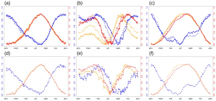
We study the potential phasing between annual T99 and W99 by analyzing the seasonal cycles of W, T, RH, and their future changes for Europe, Amazonia, and the SAA region. This analysis quantifies how seasons of highest T and highest W are phased, which only provides an estimation of the mean phasing between T99 and W99. In order to compare their seasonality and their changes, W, T, and RH are normalized between 0 and 1, subtracting the annual mean from each daily value and dividing it by the difference between annual maximum and minimum (the real values described in this section refer to Table S2). Such analyses require a model per model approach, and mean cycles over both historical and future periods for each model are cal-culated. We describe the CCSM4 seasonal cycles in the main paper (Figures 3a to 3c), since this GCM exhibits the best agreement with observations among CMIP5 models for temperature and precipitation (Knutti et al., 2013). Cycles for all of the 12 models are displayed in Figures S4, S5, and S6. Historical cycles computed using the WFDEI data set are also displayed in Figures 3d to 3f.
Figure 3. Mean seasonal cycles of W (red), T (orange), and RH (blue) over the 1979–2005 period (dashed lines) and the 2074–2100 period (solid lines) for the CCSM4 model within (a) Europe, (b) Amazonia, and (c) the Sahel to Arabia region. (d–f) Same as (a–c) but for WATCH-Forcing-Data-ERA-Interim
observations (1979–2005). Annual cycles are unitless and normalized between 0 and 1, subtracting the annual mean from each daily value and dividing it by the difference between annual maximum and minimum. Real values of W, T, and RH are displayed in Table S2.
In Europe, W, T, and RH are seasonally well correlated in both observations and GCMs (Figures 3a, 3d, and S4). The annual highest W occurs between June and August, when T is the highest (mean annual maximum = 21 K for CCSM4 in Table S2) and RH the lowest (≤ 64%), since high T drives the annual extremes of W in this region (Buzan et al., 2015). We show that highest values of T and W co-occur during summer in this region (as for northern America, not shown here). Models represent the historical mean seasonal cycles well compared to the WFDEI data set in both magnitude and phasing, except for CanESM2, IPSL-CM5A-MR, and MRI-ESM1 that simulate the annual minimum RH earlier by 1 month compared to observations (Figure S4). In the future, T increases and the associated summer RH between historical and future drops by 9%. As a consequence, this drying dampens the warming effect on the associated W99 intensification. Previous papers have shown that a larger land-ocean contrast in the lower tropospheric summer warming, as well as a faster and earlier decline of soil-moisture due to the precipitation decrease during spring, primarily drive the projected summer RH decrease in Europe (Donat et al., 2018).
Figures 3b and 3e show the seasonal cycles for the Amazon basin for CCSM4 and WFDEI and exhibit more complex cycles of W, T, and RH. During the historical period, annual highest W can occur during March-to-May and October-to-December (OND) seasons but do not co-occur with annual maximum T. The March-to-May intense W is due to both high T and high RH values, while the OND high W season is associ-ated with hotter but dryer conditions (Table S2). The seasonal cycles simulassoci-ated by the models are time-lagged compared to the observations. The spread among models is also bigger than for Europe. CCSM4 robustly represents the seasonal cycles despite dry and cold biases (Table S2). In the future, temperature increases with a preferential warming during the July-to-October (JASO) dry season. This preferential warming leads to the future occurrence of highest W values only during the OND season. However, the associated drying by −11% hampers the effect of the greater OND warming on the W increase and dampens the annual high-est W intensification in this region. This effect is illustrated by a lower increase in the seasonal variability of W compared to the variability of T (Figure 3b). No study assesses the RH variability over the Amazon basin. This variability is explained here through the analysis of precipitation variability, since the RH and precipi-tation annual cycles are seasonally well correlated in both WFDEI and GCMs (not shown here). Moreover, in the future, CMIP5 models project a negative annual mean𝛥RH, which is associated with a decrease in annual mean precipitation, soil-moisture, evaporation, and river runoff (Collins et al., 2013; Kirtman et al., 2013). Therefore, the projected greater reduction of rainfall during the JASO dry season compared to annual mean (Marengo et al., 2012) may explain the decrease of RHW99and RHT99(Table S2). It was shown in recent
decades that the warmer than average tropical Atlantic sea surface temperatures lock the Intertropical Con-vergence Zone more to the north during JASO and cause the observed drying over Amazonia (Gloor et al.,
Geophysical Research Letters
10.1029/2019GL084156
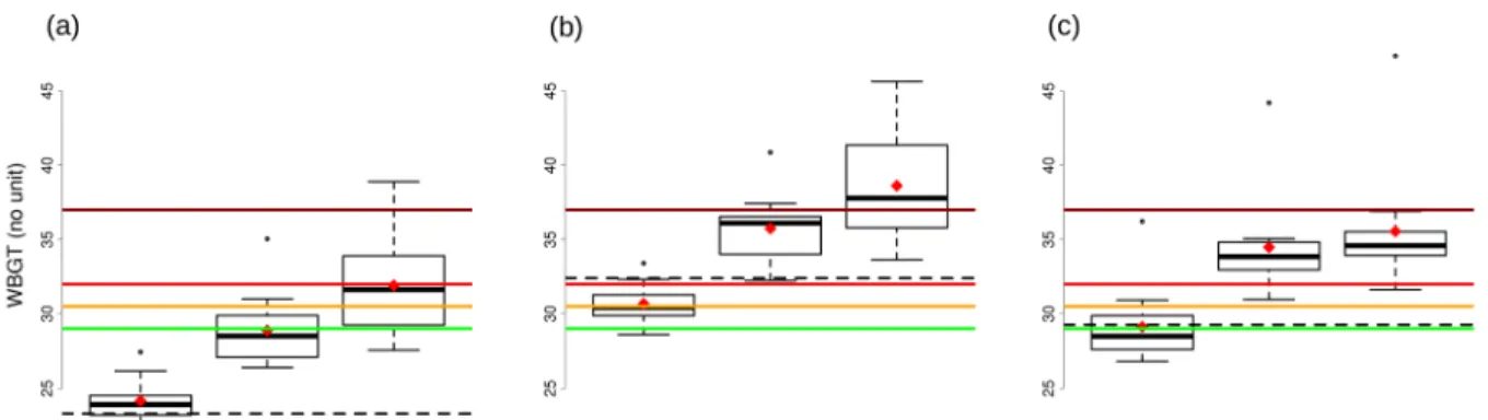
Figure 4. Boxplots of the 12 general circulation models regional mean W99 in unit of W, for (a) Europe, (b) Amazonia, and (c) the SAA region. In each panel: (left boxplot) historical W99, (middle boxplot) future projected W99, (right boxplot) theoretical future W99theo. The solid thick black lines in each boxplot represent the multimodel medians, and the red diamonds represent the multimodel means. The black dashed line in each panel corresponds to the historical WATCH-Forcing-Data-ERA-Interim mean W99. Colored lines show the risk levels of W defined in Kjellstrom et al. (2009) for a medium physical activity: 29 units of W (green line), 30.5 (orange), 32 (red), and 37 (dark red).
2015; Marengo & Espinoza, 2016; Yoon & Zeng, 2010). In the future, models simulate an accelerated sea sur-face temperatures warming over much of the tropical Atlantic, suggesting a more pronounced northward Intertropical Convergence Zone shift during JASO (Good et al., 2008). Despite large uncertainties among models, this is consistent with the projected decrease in rainfall and RH.
Within the SAA region, the season of intense W occurs in August, when the summer values of T start to decrease and the annual lowest RH starts to increase (Figures 3c and 3f). This induces a delay between annual maximum T and W from 2 weeks to 2 months depending on the models (Figure S6). Models represent T and W seasonal variabilities well but agree less for the RH cycle compared to observations, with only 5/12 models showing the annual RH bump between July and September exhibited in WFDEI (Figure 3f). At the end of the 21st century, there is no significant change in the seasonal cycle of T, and the region seems to warm homogeneously throughout the year (similar values as in Figure 1c). Nevertheless, Figure 3d shows a late summer RH increase in the future, which is consistent with the slight positive𝛥RHW99of +1–3% (Figure 2b).
In this region, the projected increase of RH enhances the warming effect on𝛥W99 and leads to the global maximum projected𝛥W99 over land. This late-summer RH increase enhancement in the future can be explained by a reinforcement of the mean moisture transports over Sahel from Atlantic and Mediterranean sources, associated with rainfall surpluses in the eastern part of the desert (Biasutti, 2013; Monerie et al., 2012). This strengthening can be favored by different mechanisms such as a greater surface warming over the continent, a northward migration, and a more intense circulation of the West African Monsoon that induces a spring drying and a fall wettening in the future (Fontaine et al., 2011; Monerie et al., 2013).
3.4. Quantification of the Effect of RH Variations on𝜟W99
To quantify the dampening/enhancing effect of𝛥RH on 𝛥W99, we compute a theoretical future mean heat stress extreme (W99theo) in a world experiencing the same global warming but no change in RH. W99theo is calculated by combining annual RHW99averaged over the 1979–2005 period and annual TW99averaged over 2074–2100. Since models locate different magnitudes of the positive/negative𝛥RHW99at different grid cells, W99theo is calculated model per model. Figure 4 displays for Europe, Amazonia, and the SAA regions the multimodel boxplots of the regional mean historical W99 values (left boxplot of each panel), the projected future W99 (middle boxplot), and the theoretical projected W99theo (right boxplot). Values for each model are shown in Figure S8.
In Europe, due to the hampering effect of the projected drying,𝛥W99 is modulated by −5.1 to +1.06 units of W depending on the model, with a multimodel median of −2.72 units (Figures 4a and S7a). We show that historical mean W99 values from the models are good compared to WFDEI observations, with a mul-timodel mean overestimation smaller than +1 unit of W. Within the Amazon basin, Figure 4b shows a dampening effect by −6.02 to −0.11 units with a multimodel median of −2.32. In this region, the models underestimate the historical W99 by −1.66 units (Figure S7b). Within the SAA region, the projected increase of W99 is modulated by −3.15 to +0.45 units of W (median = −0.66) compared to a world with no change in RH (Figures 4c and S7c). For this region, models slightly underestimate historical W99 by −0.67 units. The spread among models results from very different locations and magnitudes of the positive𝛥RHW99in
the SAA region (Figure S2), questioning whether GCMs are representing the same mechanism. As a con-sequence, some models show a negative or a slight difference between𝛥W99 and 𝛥W99theo in the SAA region due to the selected box for the regional mean (Figure S7c). However, the positive difference between
𝛥W99 and 𝛥W99theo is robust model per model and located between the Sahel, northern Africa, and
Ara-bia (Figure S8). These patterns show an enhancing effect per grid cells of 0 to +2.5 units of W due to the associated positive𝛥RHW99.
In health studies, four danger classes of heat stress were defined considering medium physical activity as 29–30.5 units of W (light danger class), 30.5–32 (moderate danger), 32–37 (strong danger), and≥37 (extreme danger) (Kjellstrom et al., 2009; Parsons, 2006). In Europe, considering these health recommendations, the green threshold is projected to be reached in 50% of the models in the future and the orange threshold in 25% (Figure 4g). Without any projected future drying (𝛥W99theo), the green danger class is reached in 70% of the GCMs, the orange class in 60%, and the red class in 50% of the models. The effect of RH variations on𝛥W99 thus plays an important role in Europe. Within the Amazon basin, future W99 reaches the most dangerous heat stress danger threshold in 30% and W99theo in 60% of the models (Figure 4h). W99 values cross the red danger class in 100% of the models even with the dampening effect of the𝛥RHW99decrease.
Moreover, in this region, the models underestimate the historical values of W99 compared to observations, which implies that projections are even worse when applying bias corrections (Dunne et al., 2013; Zhao et al., 2015). Therefore, the drying hampering effect shown can be neglected in Amazonia, since future W99 is projected to pose severe dangerous heat stress conditions for population (Kjellstrom et al., 2016). In the SAA region, future values of W99 reach the red class with or without any change in RH, and 80% of the models show an amplification effect smaller than one unit of W (Figure 4i). The global mean projected drying over land does not affect this hotspot. Indeed, the slight RHW99 increase induces the most severe global intensification of W99 by up to +6 units of W, which corresponds to an intensification stronger than the four danger classes defined for health recommendations (Figure 4).
4. Summary and Discussion
According to 12 CMIP5 models, extremes of temperature (T99) and extremes of simplified Wet-Bulb Globe Temperature (W99) tend to co-occur in mid-latitudes and to be time-lagged in the tropics due to the RH. In tropical areas, mean seasonal cycles show that extreme seasons of W occur later than extreme seasons of T by up to 2 months, when the yearly maximum temperature decreases but the RH increases. Consequently, the future changes in the corresponding W99 are not linearly correlated to the changes in T99, as suggested in Matthews et al. (2017). Significant RH changes are also projected during W99 conditions in the future and modulate the global warming effect on𝛥W99 in all regions. The global maximum W99 intensification over land is located within the Sahel to Arabia region, where the slight positive RH changes enhances𝛥W99, and within the Amazon basin, where the drying effect hampers the W99 intensification.
Nevertheless, robustness in the𝛥RH projections during W99 among models is limited. The significance is better over drying areas (Figure S2), consistent with seasonal and annual mean changes in RH (not shown here). These uncertainties may be explained by the relative contribution of processes driving the changes in variability such as enhanced land-atmosphere coupling, reduction in cloudiness, and atmospheric circula-tion changes that strongly differ among CMIP5 models (Deser et al., 2012; Flato et al., 2013). In particular, the SAA region emphasized in this paper would deserve a further investigation to understand the multimodel differences.
The multimodel analysis conducted here shows a good representation of historical mean values and seasonal variabilities of W, T, and RH compared to the WFDEI observations. However, model biases in extremes are well known compared to observations and reanalyses (Dunne et al., 2013; Fischer & Knutti, 2013; Zhao et al., 2015), and bias corrections would be necessary to quantify the𝛥RH impact on human health and labor productivity. When using the simplified W, we also neglect the solar radiation and wind components in assessing the changes in heat stress extremes (Grundstein & Cooper, 2018). This approximation may impact the implications of the changes on the labor productivity and health (Kjellstrom et al., 2009).
These results, not diminishing the severe conclusions of the projected increase in temperature, confirm the importance of studying humidity variations. They highlight the need to fill the lack of high-quality observations that still limits confidence for both observed and projected changes (Chen et al., 2018). They also exhibit the need to better represent the hydrological cycle and atmospheric circulation in GCMs.
Geophysical Research Letters
10.1029/2019GL084156
Land-atmosphere feedbacks play an important role in the assessment of climate impacts on population (Seneviratne et al., 2018). They induce moisture fluxes between soil and atmosphere, modulating the occur-rence of heat extremes in the mid-latitudes, where they particularly determine the onset of heat waves through larger-scale circulation patterns (Horton et al., 2016; Seneviratne et al., 2006). Atmospheric circula-tion also needs to be better constrained in GCMs, since climate extremes in tropical regions such as droughts can directly be linked with moisture transport from ocean and circulation strengthening (Barichivich et al., 2018).Following the time lag emphasized in the tropics, temperature and heat stress extremes should be analyzed as consecutive events during the year in order to improve the assessment of the future climate change-driven impacts on population (Leonard et al., 2014; Mora et al., 2018; Zscheischler et al., 2018).
References
Alexander, L. V., Zhang, X., Peterson, T. C., Caesar, J., Gleason, B., Klein Tank, A. M. G., et al. (2006). Global observed changes in daily climate extremes of temperature and precipitation. Journal of Geophysical Research, 111, D05109. https://doi.org/10.1029/2005JD006290 Australian Bureau of Meteorology (2010). The wet bulb globe temperature (wbgt). Retrieved from http://bom.gov.au/info/thermalstress Barichivich, J., Gloor, E., Peylin, P., Brienen, R. J. W., Schöngart, J., Espinoza, J. C., & Pattnayak, K. C. (2018). Recent intensification of
Amazon flooding extremes driven by strengthened Walker circulation. Science Advances, 4(9), eaat8785. https://doi.org/10.1126/sciadv. aat8785
Biasutti, M. (2013). Forced Sahel rainfall trends in the CMIP 5 archive. Journal of Geophysical Research: Atmospheres, 118, 1613–1623. https://doi.org/10.1002/jgrd.50206
Bowler, K. (2005). Acclimation, heat shock and hardening. Journal of Thermal Biology, 30(2), 125–130. https://doi.org/10.1016/j.jtherbio. 2004.09.001
Buzan, J. R., Oleson, K., & Huber, M. (2015). Implementation and comparison of a suite of heat stress metrics within the Community Land Model version 4.5. Geoscientific Model Development, 8(2), 151–170. https://doi.org/10.5194/gmd-8-151-2015
Chavaillaz, Y., Joussaume, S., Bony, S., & Braconnot, P. (2016). Spatial stabilization and intensification of moistening and drying rate patterns under future climate change. Climate Dynamics, 47(3-4), 951–965. https://doi.org/10.1007/s00382-015-2882-9
Chen, Y., Moufouma-Okia, W., Masson-Delmotte, V. Ã., Zhai, P., & Pirani, A. (2018). Recent progress and emerging topics on weather and climate extremes since the fifth assessment report of the intergovernmental panel on climate change. Annual Review of Environment
and Resources, 43(1), 35–59. https://doi.org/10.1146/annurev-environ-102017-030052
Collins, M., Knutti, R., Arblaster, J., Dufresne, J.-L., Fichefet, T., Friedlingstein, P., et al. (2013). Long-term climate change: Projections, commitments and irreversibility. In T. F. Stocker, D. Qin, G.-K. Plattner, M. Tignor, S. K. Allen, J. Boschung, A. Nauels, Y. Xia, V. Bex, & P. M. Midgley (Eds.), Climate change 2013: The physical science basis. contribution of working group i to the fifth assessment report
of the intergovernmental panel on climate change(pp. 1029–1136). Cambridge, United Kingdom and New York, NY, USA: Cambridge University Press. https://doi.org/10.1017/CBO9781107415324.024
Davies-Jones, R. (2008). An efficient and accurate method for computing the Wet-Bulb temperature along pseudoadiabats. Monthly Weather
Review, 136(7), 2764–2785. https://doi.org/10.1175/2007MWR2224.1
Deser, C., Phillips, A., Bourdette, V., & Teng, H. (2012). Uncertainty in climate change projections: The role of internal variability. Climate
Dynamics, 38(3-4), 527–546. https://doi.org/10.1007/s00382-010-0977-x
Diffenbaugh, N. S., Pal, J. S., Giorgi, F., & Gao, X. (2007). Heat stress intensification in the Mediterranean climate change hotspot.
Geophysical Research Letters, 34, L11706. https://doi.org/10.1029/2007GL030000
Donat, M. G., Pitman, A. J., & Angélil, O. (2018). Understanding and reducing future uncertainty in midlatitude daily heat extremes via land surface feedback constraints. Geophysical Research Letters, 45, 10,627–10,636. https://doi.org/10.1029/2018GL079128
Dunne, J. P., Stouffer, R. J., & John, J. G. (2013). Reductions in labour capacity from heat stress under climate warming. Nature Climate
Change, 3(6), 563–566. https://doi.org/10.1038/nclimate1827
Fischer, E. M., & Knutti, R. (2013). Robust projections of combined humidity and temperature extremes. Nature Climate Change, 3(2), 126–130. https://doi.org/10.1038/nclimate1682
Fischer, E. M., Oleson, K. W., & Lawrence, D. M. (2012). Contrasting urban and rural heat stress responses to climate change. Geophysical
Research Letters, 39, L03705. https://doi.org/10.1029/2011GL050576
Fischer, E. M., & Schar, C. (2010). Consistent geographical patterns of changes in high-impact European heatwaves. Nature Geoscience,
3(6), 398–403. https://doi.org/10.1038/ngeo866
Flato, G., Marotzke, J., Abiodun, B., Braconnot, P., Chou, S. C., Collins, W., et al. (2013). Evaluation of climate models. In T. F. Stocker, D. Qin, G.-K. Plattner, M. Tignor, S. K. Allen, J. Boschung, A. Nauels, Y. Xia, V. Bex, & P. M. Midgley (Eds.), Climate change 2013: The
physical science basis. contribution of working group i to the fifth assessment report of the intergovernmental panel on climate change(pp. 741–8). Cambridge, United Kingdom and New York, NY, USA: Cambridge University Press. https://doi.org/10.1017/ CBO9781107415324.020
Fontaine, B., Roucou, P., & Monerie, P.-A. (2011). Changes in the African monsoon region at medium-term time horizon using 12 AR4 coupled models under the A1b emissions scenario. Atmospheric Science Letters, 12(1), 83–88. https://doi.org/10.1002/asl.321 Gloor, M., Barichivich, J., Ziv, G., Brienen, R., Schöngart, J., Peylin, P., et al. (2015). Recent Amazon climate as background for possible
ongoing and future changes of Amazon humid forests: Amazon climate and tropical forests. Global Biogeochemical Cycles, 29, 1384–1399. https://doi.org/10.1002/2014GB005080
Good, P., Lowe, J. A., Collins, M., & Moufouma-Okia, W. (2008). An objective tropical Atlantic sea surface temperature gradient index for studies of south Amazon dry-season climate variability and change. Philosophical Transactions of the Royal Society B: Biological Sciences,
363(1498), 1761–1766. https://doi.org/10.1098/rstb.2007.0024
Grundstein, A., & Cooper, E. (2018). Assessment of the Australian Bureau of Meteorology wet bulb globe temperature model using weather station data. International Journal of Biometeorology, 62(12), 2205–2213. https://doi.org/10.1007/s00484-018-1624-1
Hirschi, M., Seneviratne, S. I., Alexandrov, V., Boberg, F., Boroneant, C., Christensen, O. B., et al. (2011). Observational evidence for soil-moisture impact on hot extremes in southeastern Europe. Nature Geoscience, 4(1), 17–21. https://doi.org/10.1038/ngeo1032
Acknowledgments
CMIP5 data used in this paper are freely available at https://esgf-node. llnl.gov/projects/cmip5/. We acknowledge the World Climate Research Programme's Working Group on Coupled Modelling, which is in charge of the fifth Coupled Model Intercomparison Project, and we thank the climate modelling groups for producing and making available their model output. To analyze the CMIP5 data, this study benefited from the IPSL Prodiguer-Ciclad facility which is supported by CNRS, UPMC, Labex L-IPSL which is funded by the ANR (Grant ANR-10-LABX-0018) and by the European FP7 IS-ENES2 project (Grant 312979). We warmly acknowledge P. Braconnot, N. De Noblet, and R. Vautard at LSCE-IPSL for their comments and useful advices on our study. We thank C. Iles for her professional english revision. We thank the two anonymous reviewers for their helpful suggestions and comments.
Horton, R. M., Mankin, J. S., Lesk, C., Coffel, E., & Raymond, C. (2016). A review of recent advances in research on extreme heat events.
Current Climate Change Reports, 2, 242–259. https://doi.org/10.1007/s40641-016-0042-x
Kirtman, B., Power, S. B., Adedoyin, J. A., Boer, G. J., Bojariu, R., Camilloni, I., et al. (2013). Near-term climate change: Projections and predictability. In T. F. Stocker, D. Qin, G.-K. Plattner, M. Tignor, S. K. Allen, J. Boschung, A. Nauels, Y. Xia, V. Bex, & P. M. Midgley (Eds.),
Climate change 2013: The physical science basis. Contribution of working group i to the fifth assessment report of the intergovernmental panel on climate change(pp. 9531028). Cambridge, United Kingdom and New York, NY, USA: Cambridge University Press. https://doi. org/10.1017/CBO9781107415324.023
Kjellstrom, T., Briggs, D., Freyberg, C., Lemke, B., Otto, M., & Hyatt, O. (2016). Heat, human performance, and occupational health: A key issue for the assessment of global climate change impacts. Annual Review of Public Health, 37(1), 97–112. https://doi.org/10.1146/ annurev-publhealth-032315-021740
Kjellstrom, T., Holmer, I., & Lemke, B. (2009). Workplace heat stress, health and productivity – an increasing hallenge for low and middle-income countries during climate change. Global Health Action, 2(1), 2047. https://doi.org/10.3402/gha.v2i0.2047
Knutti, R., Masson, D., & Gettelman, A. (2013). Climate model genealogy: Generation CMIP 5 and how we got there. Geophysical Research
Letters, 40, 1194–1199. https://doi.org/10.1002/grl.50256
Leonard, M., Westra, S., Phatak, A., Lambert, M., van den Hurk, B., McInnes, K., et al. (2014). A compound event framework for understanding extreme impacts: A compound event framework. Wiley Interdisciplinary Reviews: Climate Change, 5(1), 113–128. https:// doi.org/10.1002/wcc.252
Marengo, J. A., Chou, S. C., Kay, G., Alves, L. M., Pesquero, J. F., Soares, W. R., et al. (2012). Development of regional future climate change scenarios in South America using the Eta CPTEC/HadCM3 climate change projections: Climatology and regional analyses for the Amazon, So Francisco and the Paran River basins. Climate Dynamics, 38(9-10), 1829–1848. https://doi.org/10.1007/s00382-011-1155-5 Marengo, J. A., & Espinoza, J. C. (2016). Extreme seasonal droughts and floods in Amazonia: Causes, trends and impacts: Extremes in
amazonia. International Journal of Climatology, 36(3), 1033–1050. https://doi.org/10.1002/joc.4420
Matthews, TomK. R., Wilby, R. L., & Murphy, C. (2017). Communicating the deadly consequences of global warming for human heat stress. Proceedings of the National Academy of Sciences, 114(15), 3861–3866. https://doi.org/10.1073/pnas.1617526114
Meehl, G. A. (2004). More intense, more frequent, and longer lasting heat waves in the 21st century. Science, 305(5686), 994–997. https:// doi.org/10.1126/science.1098704
Monerie, P.-A., Fontaine, B., & Roucou, P. (2012). Expected future changes in the African monsoon between 2030 and 2070 using some CMIP 3 and CMIP 5 models under a medium-low RCP scenario. Journal of Geophysical Research, 117, D16111. https://doi.org/10.1029/ 2012JD017510
Monerie, P.-A., Roucou, P., & Fontaine, B. (2013). Mid–century effects of climate change on African monsoon dynamics using the A1b emission scenario. International Journal of Climatology, 33(4), 881–896. https://doi.org/10.1002/joc.3476
Mora, C., Dousset, B., Caldwell, I. R., Powell, F. E., Geronimo, R. C., Bielecki, C, et al. (2017). Global risk of deadly heat. Nature Climate
Change, 7(7), 501–506. https://doi.org/10.1038/nclimate3322
Mora, C., Spirandelli, D., Franklin, E. C., Lynham, J., Kantar, M. B., Miles, W., et al. (2018). Broad threat to humanity from cumulative climate hazards intensified by greenhouse gas emissions. Nature Climate Change, 8(12), 1062–1071. https://doi.org/10.1038/ s41558-018-0315-6
Parsons, K. (2006). Heat stress standard ISO 7243 and its global application. Industrial Health, 44(3), 368–379.
Screen, J. A., & Simmonds, I. (2010). Increasing fall-winter energy loss from the Arctic Ocean and its role in Arctic temperature amplification: Increasing Arctic heat loss. Geophysical Research Letters, 37, L16707. https://doi.org/10.1029/2010GL044136
Seneviratne, S. I., Lüthi, D., Litschi, M., & Schär, C. (2006). Land-atmosphere coupling and climate change in Europe. Nature, 443(7108), 205–209. https://doi.org/10.1038/nature05095
Seneviratne, S. I., Wartenburger, R., Guillod, B. P., Hirsch, A. L., Vogel, M. M., Brovkin, V., et al. (2018). Climate extremes, land-climate feedbacks and land-use forcing at 1.5◦C. Philosophical Transactions of the Royal Society A: Mathematical, Physical and Engineering
Sciences, 376(2119), 20160450. https://doi.org/10.1098/rsta.2016.0450
Taylor, K. E., Stouffer, R. J., & Meehl, G. A. (2012). An overview of CMIP 5 and the experiment design. Bulletin of the American Meteorological
Society, 93(4), 485–498. https://doi.org/10.1175/BAMS-D-11-00094.1
Vogel, M. M., Orth, R., Cheruy, F., Hagemann, S., Lorenz, R., Hurk, B. J. J. M., & Seneviratne, S. I. (2017). Regional amplification of projected changes in extreme temperatures strongly controlled by soil moisture–temperature feedbacks. Geophysical Research Letters,
44, 1511–1519. https://doi.org/10.1002/2016GL071235
Weedon, G. P., Balsamo, G., Bellouin, N., Gomes, S., Best, M. J., & Viterbo, P. (2014). The WFDEI meteorological forcing data set: WATCH Forcing Data methodology applied to ERA-Interim reanalysis data. Water Resources Research, 50, 7505–7514. https://doi.org/10.1002/ 2014WR015638
Yaglou, C. P., & Minard, D. (1957). Control of heat casualties at militarytraining centers, American medical association archives of in-dustrial health, 16, 3020–316.
Yoon, J.-H., & Zeng, N. (2010). An Atlantic influence on Amazon rainfall. Climate Dynamics, 34(2-3), 249–264. https://doi.org/10.1007/ s00382-009-0551-6
Zhao, Y., Ducharne, A., Sultan, B., Braconnot, P., & Vautard, R. (2015). Estimating heat stress from climate-based indicators: Present-day biases and future spreads in the CMIP5 global climate model ensemble. Environmental Research Letters, 10(8), 84013. https://doi.org/ 10.1088/1748-9326/10/8/084013
Zscheischler, J., Westra, S., van den Hurk, B. J. J. M., Seneviratne, S. I., Ward, P. J., Pitman, A., et al. (2018). Future climate risk from compound events. Nature Climate Change, 8(6), 469–477. https://doi.org/10.1038/s41558-018-0156-3