Interannual variability in tropospheric nitrous oxide

(1)

HAL Id: hal-02930028

https://hal.archives-ouvertes.fr/hal-02930028

Submitted on 17 Sep 2020

HAL is a multi-disciplinary open access

archive for the deposit and dissemination of sci-entific research documents, whether they are pub-lished or not. The documents may come from teaching and research institutions in France or abroad, or from public or private research centers.

L’archive ouverte pluridisciplinaire HAL, est destinée au dépôt et à la diffusion de documents scientifiques de niveau recherche, publiés ou non, émanant des établissements d’enseignement et de recherche français ou étrangers, des laboratoires publics ou privés.

Interannual variability in tropospheric nitrous oxide

R. Thompson, E. Dlugokencky, F. Chevallier, P. Ciais, G. Dutton, J. Elkins,

R. Langenfelds, R. Prinn, R. Weiss, Y. Tohjima, et al.

To cite this version:

R. Thompson, E. Dlugokencky, F. Chevallier, P. Ciais, G. Dutton, et al.. Interannual variability in tropospheric nitrous oxide. Geophysical Research Letters, American Geophysical Union, 2013, 40 (16), pp.4426-4431. �10.1002/grl.50721�. �hal-02930028�

(2)

Interannual variability in tropospheric nitrous oxide

R. L. Thompson,1E. Dlugokencky,2F. Chevallier,3P. Ciais,3G. Dutton,2J. W. Elkins,2 R. L. Langenfelds,4R. G. Prinn,5R. F. Weiss,6Y. Tohjima,7S. O’Doherty,8

P. B. Krummel,4P. Fraser,4and L. P. Steele4

Received 18 March 2013; revised 26 June 2013; accepted 2 July 2013; published 27 August 2013.

[1] Observations of tropospheric N2O mixing ratio show

signiﬁcant variability on interannual timescales (0.2 ppb, 1 standard deviation). We found that interannual variability in N2O is weakly correlated with that in CFC-12 and SF6

for the northern extratropics and more strongly correlated for the southern extratropics, suggesting that interannual variability in all these species is inﬂuenced by large-scale atmospheric circulation changes and, for SF6in particular,

interhemispheric transport. N2O interannual variability

was not, however, correlated with polar lower stratospheric temperature, which is used as a proxy for stratosphere-to-troposphere transport in the extratropics. This suggests that stratosphere-to-troposphere transport is not a dominant factor in year-to-year variations in N2O

growth rate. Instead, we found strong correlations of N2O

interannual variability with the Multivariate ENSO Index. The climate variables, precipitation, soil moisture, and temperature were also found to be signiﬁcantly correlated with N2O interannual variability, suggesting that climate-driven

changes in soil N2O ﬂux may be important for variations in

N2O growth rate. Citation: Thompson, R. L., et al. (201 ),

Interannual variability in tropospheric nitrous oxide, Geophys. Res. Lett., 40, 4426–4431, doi:10.1002/grl.50721.

1. Introduction

[2] Nitrous oxide (N2O) is now the third most important

long-lived anthropogenic greenhouse gas. N2O is also an

important ozone-depleting substance (ODS), as it reacts with O(1D) to produce NO in the stratosphere, and currently the ozone-depleting potential-weighted emissions of N2O are

considered the largest of any ODS [Ravishankara et al.,

2009]. The atmospheric mixing ratio of N2O has been

increasing strongly since the preindustrial era largely as the result of human activities, namely the increasing input of reactive nitrogen into ecosystems (predominantly by N fertilizer use), which accelerates denitriﬁcation rates and enhances N2O emissions from soils and coastal waters to

the atmosphere [Syakila and Kroeze, 2011].

[3] Atmospheric observations of N2O began in the early

1970s and have revealed a steady quasi-linear increase in concentrations since then [Prinn et al., 1990]. Superimposed on this long-term trend are seasonal and interannual variations. The seasonal variability in N2O mixing ratio is determined by

the combined effect of transport and surface ﬂuxes. Of particular importance is stratosphere-to-troposphere transport (STT), which brings air with a low N2O mixing ratio from

the stratosphere into the troposphere. STT has a maximum in spring in the Northern Hemisphere and is particularly important in deﬁning the seasonal cycle in middle to high latitudes [Ishijima et al., 2010; Nevison et al., 2004; Nevison et al., 2007; Nevison et al., 2011]. The interannual variability in N2O mixing ratio has only been investigated in a few

studies [Ishijima et al., 2009; Nevison et al., 2007; Nevison et al., 2011], which has partly been due to the limited availability of long-term measurements of N2O precise

enough to be used for this purpose. In the late 1990s and early 2000s, measurements of N2O began at a number of new sites

and provide measurements precise enough to be used for such a study. Previous investigations have pointed to an important role of STT in N2O interannual variability [Nevison et al.,

2007; Nevison et al., 2011]. This is based on the observed correlation between anomalies in N2O minima at middle- to

high-latitude sites and anomalies in polar lower stratospheric temperature (PLST), which is used as a proxy for the strength of the Brewer-Dobson circulation and STT [Huck et al., 2005; Waugh et al., 1999].

[4] Here we examine tropospheric N2O from 1996 to 2009

to better understand the importance of atmospheric transport and surfaceﬂux variability on N2O interannual variability.

We exploit a data set encompassing 30ﬂask and 6 in situ sites (see Table S1 in the supporting information) and utilize observations of two other atmospheric trace gases, CFC-12 (CF2Cl2) and SF6, which are useful tracers for atmospheric

transport and have been previously used in investigating seasonal variability in N2O [Nevison et al., 2007].

2. Observations and Model

[5] Approximately weekly N2O measurements from

dis-crete air samples (ﬂasks) are used from the NOAA CCGG (Carbon Cycle Greenhouse Gases group) (E. Dlugokencky et al., in preparation, 2013) and the Commonwealth Scientiﬁc and Industrial Research Organisation (CSIRO)

Additional supporting information may be found in the online version of this article.

1

Norwegian Institute for Air Research, Kjeller, Norway.

2_{Global Monitoring Division, Earth System Research Laboratory}

(ESRL), National Oceanic and Atmospheric Administration, Boulder, Colorado, USA.

3

Laboratoire des Sciences du Climat et de l’Environnement, Gif-sur-Yvette, France.

4

Centre for Australian Weather and Climate Research/Commonwealth Scientiﬁc and Industrial Research Organisation, Aspendale, Victoria, Australia.

5

Massachusetts Institute of Technology, Cambridge, Massachusetts, USA.

6

Scripps Institution of Oceanography, University of California, San Diego, La Jolla, California, USA.

7

National Institute for Environmental Studies, Tsukuba, Japan.

8_{University of Bristol, Bristol, United Kingdom.}

0094-8276/13/10.1002/grl.50721

(3)

[Francey et al., 2003] global networks. In situ measurements are used from AGAGE (Advanced Global Atmospheric Gases Experiment) [Prinn et al., 2000] and NIES (National Institute for Environmental Studies) sites [Tohjima et al., 2000] (see Table S1 in the supporting information). For AGAGE sites, the data are available at 40 min intervals while for NIES sites, the data are available as daily averages. Flask and in situ measurements are made using gas chromatographs ﬁtted with electron capture detectors (GC-ECD) and are reported as dry air mole fractions (nmol mol 1_{, abbreviated}

ppb). NOAA and CSIRO data are reported on the NOAA-2006A scale [Hall et al., 2007], while AGAGE and NIES data are reported on the SIO-1998 and NIES scales, respectively. AGAGE data were adjusted to the NOAA-2006A scale by comparing measurements at sites where AGAGE and NOAA operate in parallel, while NIES data were adjusted based on the results of intercomparisons of standards (Δχ = 0.6 ppb, Y. Tohjima, personal communication, 2012). There is some concern that there may be a calibration shift between CCGG N2O data collected before and after 2001. For this reason, we

run our analyses twice, ﬁrst using all available sites and, second, using a subset of sites (“core” sites), which excludes CCGG sites and sites with large data gaps (>6 months) (see Table S1). CFC-12 and SF6measurements are fromﬂasks in

the NOAA HATS (Halocarbons and other Atmospheric Trace Species) network and in situ instruments in the AGAGE network. Both measurements are made using GC-ECD and presented as dry air mole fractions (pmol mol 1_{, abbreviated}

ppt). CFC-12 measurements are reported monthly on the NOAA-2008 (HATS) and SIO-2005 (AGAGE) scales and SF6 measurements on the NOAA-2006 (HATS) and

SIO-2005 (AGAGE) scales.

[6] Interannual variability (IAV) was calculated for N2O at

each site used in this study by first subtracting the multiannual trend,fitted as a second-order polynomial, and then applying a low-pass Butterworthfilter (fourth order) to the residuals tofilter seasonal and higher-frequency signals. Two passes of thefilter (forward and reverse) were applied to correct for any phase distortion. This method was chosen preferentially over methods that involve fitting a seasonal cycle to the data (e.g., based on harmonic curves) since at many sites the seasonality has small amplitude and/or is irregular. Our definition of IAV is the component of the signal with periodicities longer than 12 months and is closely correlated with the growth rate. The Butterworth filter has been used previously to examine IAV in atmospheric species, e.g., in the studies of Ishijima et al. [2009] and Nakazawa et al. [1997]. Both methods, however, were tested and gave consistent results. The same method was applied to CFC-12 and SF6, but for CFC-12 a third-order polynomial

was used toﬁt the multiannual trend.

[7] Atmospheric simulations of N2O were performed using

the Laboratoire de Météorologie Dynamique general circula-tion model (LMDz, version 4) [Hourdin et al., 2006], which includes N2O photolysis and oxidation reactions in the

stratosphere and has an N2O lifetime of approximately

120 years which is within the range of recent estimates of 131 ± 10 years [Prather et al., 2012]. LMDz has a horizontal resolution of 3.75° longitude × 2.5° latitude and 19 hybrid pressure levels up to 3 hPa. Modeled transport was nudged to European Centre for Medium-Range Weather Forecasts (ECMWF) ERA-40 wind ﬁelds at 6-hourly intervals. The model was run with climatological monthly

N2O emission estimates comprising natural and

agricul-tural soilﬂuxes, ocean ﬂuxes, as well as biomass burning and anthropogenic (nonagricultural) emissions (for details see the supporting information).

3. Results and Discussion

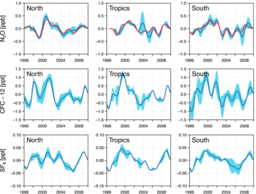
[8] IAV in N2O, CFC-12, and SF6is shown for the tropics

and the northern and southern extratropics from 1996 to 2009 (Figure 1). The standard deviation of N2O IAV is

approxi-mately 0.2 ppb and is signiﬁcant compared to the variability across all sites used within each region (for details see Table S2). N2O IAV is weakly correlated with CFC-12

IAV in the northern extratropics, more strongly correlated in the southern extratropics, and uncorrelated in the tropics (see Table 1). CFC-12, like N2O, is only lost by

photochem-ical reactions in the stratosphere and has a similar lifetime to N2O (108 years [Rigby et al., 2012]). This, and given that

there is little seasonal and interannual variability in CFC-12 emissions, means that it is a pertinent tracer for the inﬂuence of STT. The fact that IAV in N2O and CFC-12 is only weakly

correlated in the northern extratropics suggests that STT is not the dominant factor in N2O variability at these latitudes.

IAV in N2O and SF6is also only weakly correlated in the

northern extratropics but is more strongly correlated in the tropics and southern extratropics. SF6is a very long-lived

species (lifetime of 3200 years [Ravishankara et al., 1993]) with no loss in the stratosphere, making variations in the tro-pospheric mixing ratio less sensitive to STT than, e.g., N2O

or CFC-12. In addition, its emissions have little seasonal or interannual variability, making it a useful tracer for tropo-spheric transport. Emissions of SF6 are predominantly in

the Northern Hemisphere and SF6has a strong north-south

concentration gradient. Therefore, the correlation of IAV in N2O with that of SF6in the southern extratropics likely

re-sults from variations in interhemispheric transport.

[9] Anomalies in N2O seasonal minima at a number of

middle- and high-latitude sites are correlated with anomalies in PLST (used as a proxy for STT) as shown by Nevison et al. [2011]. However, we alsoﬁnd substantial variability in the N2O maxima, which is not correlated with variability in the

N2O minima and cannot be explained by STT alone.

Comparing N2O IAV (which is sensitive to anomalies in both

the maxima and minima) in the northern (southern) extratropics with Arctic (Antarctic) PLST, weﬁnd no signif-icant correlation (see Table S3). This indicates that STT alone cannot explain the observed IAV in N2O in the middle

to high latitudes. Another test for the inﬂuence of STT is to look at the magnitude of this effect. Following Nevison et al. [2007], we estimate the change in tropospheric N2O

mixing ratio from variations in STT on interannual time-scales. Assuming annually balanced upward and downward air massﬂuxes, a N2O cross-tropopause gradient of 20 ppb,

and a net global downward ﬂux of between 4 × 109 _and

11.6 × 109kg s 1 (median of 5.9 × 109kg s 1, n = 3) [Gettelman et al., 1997; Schoeberl, 2004] with a 20% interannual variation (this number is very uncertain [Schoeberl, 2004]) results in a range of 0.5–1.4 yr 1

interannual variation in the tropospheric mass of N2O. This

equates to 0.11–0.32 ppb IAV in the N2O tropospheric

mixing ratio, of which only the upper limit (i.e., 0.32 ppb) would have about the right magnitude to explain the observed IAV.

(4)

[10] Examining the latitudinal pattern of N2O IAV, weﬁnd

that there is a strong tropical and subtropical signal that is closely in phase across hemispheres and which is negatively correlated with the Multivariate ENSO Index (MEI) (http:// www.esrl.noaa.gov/psd/enso/mei/) such that negative N2O

anomalies coincide with El Niño conditions (see Figure 2). A correlation of N2O IAV with ENSO has been previously

detected in long-term N2O shipboard measurements in the

northern and western Paciﬁc [Ishijima et al., 2009] and from in situ measurements at Samoa [Nevison et al., 2007]. We ﬁnd the strongest correlation with a lag time of between 7 and 9 months in the tropics (R = 0.61) and southern extratropics (R = 0.59), and between 9 and 11 months in the northern extratropics (R = 0.67, see Table 1). In the tropics, CFC-12 IAV (at Samoa) is also correlated with ENSO (R = 0.41). Changes in interhemispheric transport, which is affected by ENSO-driven changes in circulation, has been suggested as a mechanism for this correlation and has been observed for other species at Samoa (e.g., methane and methylchloroform) [Hartley and Black, 1995; Prinn et al., 1992]. For N2O the IAV is closely in phase for both

hemispheres; however, if changes in interhemispheric

transport were mainly responsible for the IAV, then the signal in each hemisphere should be out of phase [Steele et al., 1992]. Also, for species with strong biogenic sources, such as N2O, this correlation may be partly due to variability

in the emissions related to ENSO-driven climate changes. We examine the inﬂuence of tropospheric transport and emission variability on N2O IAV in the following paragraphs.

[11] The transport inﬂuence on tropospheric N2O

variabil-ity was modeled using LMDz, and time series for each site were extracted from the 4-D simulated N2O mixing ratios

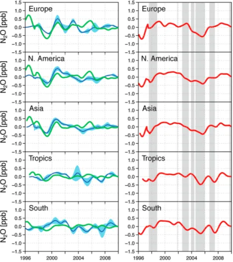
and analyzed in the same way as the observations (see section above). IAV at different sites were then averaged in ﬁve geographical regions (see Table S2). Our model (which does not account for IAV in N2O emissions) captures about 40%

of the observed variation in IAV in extratropical regions and none in the tropics (see Figure 3). Simulations using IAV in the emissions (not shown) did not perform better owing to large uncertainties in the emission variability. The model-observation difference for all regions may be partly due to model transport errors, but on the basis of comparisons with CFC-12, for which the agreement is much better (R = 0.57 for the northern extratropics and R = 0.47 for the

Table 1. Correlation of N2O IAV With That of the Trace Gases, CFC-12 and SF6, and With MEIa

Region

Correlation With Tracer Gases Correlation With MEI

CFC-12 SF6 Months of Highest Correlation Correlation Coefﬁcient

Northern extratropics 0.37 0.35 9–11 0.67

Tropics (0.25) 0.51 7–9 0.61

Southern extratropics 0.68 0.67 7–9 0.59

a

All correlations were signiﬁcant at the 0.05 level, except the correlation of N2O with CFC-12 in the tropics, which is, therefore, shown in parentheses. The

correlation with MEI is shown for the lag times (in months) that gave the highest correlation. The negative correlation means that El Niño events are correlated with negative N2O anomalies.

Figure 1. IAV of N2O, CFC-12, and SF6shown for northern (North) and southern (South) extratropical and tropical regions.

The solid blue curve is the mean and the shaded blue area is the standard deviation of IAV calculated at all sites. For N2O, the

(5)

tropics, see Table S4), this error is likely to be much less important than the inﬂuence of IAV in the emissions. The model-observation comparison suggests that the inﬂuence of tropospheric transport is important for N2O IAV in the

extratropics; however, it appears to be less important in the tropics.

[12] Figure 3 shows the IAV in tropospheric N2O mixing

ratios attributed to changes in N2O emissions (i.e., the

observed IAV minus the simulated IAV due to the influence of transport). Denitrification (and to a lesser extent nitrifica-tion) in soils is the primary source of N2O. These processes

are known to be very sensitive to soil moisture and tempera-ture, precipitation, soil type, soil pH, and nitrogen substrate availability [Davidson, 1993; Skiba and Smith, 2000; Smith et al., 1998]. We performed an analysis of variance and a correlation analysis of N2O IAV with the independent

variables: soil moisture and temperature, and precipitation (ECMWF ERA-Interim, for details see supporting informa-tion), which vary substantially on annual timescales. ERA-Interim soil moisture has been previously evaluated against in situ data (correlation of 0.63 for 2008 to 2010) [Albergel et al., 2012]. The analyses were performed on N2O IAV data

with and without the correction for the inﬂuence of transport. Due to potential errors in the modeled transport, we refer only to regions where both analyses gave consistent results (see Tables S5 and S6). For Europe, soil temperature and precipitation were positively correlated with N2O IAV.

With the correction for the inﬂuence of transport, soil moisture was also positively correlated, and the correlation coefﬁcients increased for all variables. For the tropics, the correlation was calculated with the independent variables for South America, Africa, and Asia, separately. In contrast to Europe, N2O IAV was negatively correlated with

temper-ature, a result that is consistent with that of Ishijima et al. [2009] who found a negative correlation between N2O IAV

and soil temperature in the Northern Hemisphere. N2O IAV

in the tropics was positively correlated with soil moisture (also consistent with Ishijima et al. [2009]). The opposing signs of correlation with soil moisture and temperature in the tropics may be a reﬂection of the fact that anomalies in soil moisture and temperature are often negatively correlated. [13] A number of extreme climatic events are associated

with signiﬁcant changes in N2O mixing ratio. The

European drought in 2003 produced a strong negative soil moisture anomaly, which coincides with the onset of a signif-icant decrease in N2O over Europe, which is not observed in

either North America or Asia (see Figure S4). In summer 2003, a persistent high-pressure system led to stable conditions and longer air mass residence times over Europe [Solberg et al., 2008]. Thus, if no change in surface emissions is assumed, transport alone would result in increased N2O mixing ratio, while the opposite is observed.

Sustained periods of low soil moisture in 2005 and in theﬁrst half of 2007 in Asia and South America also coincide with negative N2O anomalies in the tropical signal, while above

average soil water content in 2003 and 2008 in Asia and Africa coincides with positive N2O anomalies. The years

2005 and 2007 (ﬁrst half only) are associated with El Niño, which typically brings drier and warmer conditions to South America, Southeast Asia, and South Africa, especially during the Northern Hemisphere winter, whereas 2003 was nearly neutral, and the second half of 2007 and 2008 were La Niña years, which brings generally cooler and wetter con-ditions to the same regions [Trenberth et al., 1998].

[14] Interannual variability in N2O soil emissions has been

previously linked to variations in soil moisture and precipita-tion, particularly in the tropics [Potter et al., 1996; Werner et al., 2007], and in soil temperature, particularly in temperate regions [Potter et al., 1996]. Low soil moisture limits the pro-duction of N2O via denitriﬁcation [Bouwman, 1998] and may

Figure 2. (top) IAV of N2O (ppb) interpolated with latitude and time. Data were calculated using a bivariate linear

interpo-lation (15° spatial and monthly temporal resolution) of the IAV calculated for each of the 36 sites. The dashed gray lines indicate the latitudinal extent of the stations used in the calculation of the tropical signal. (bottom) MEI shown at monthly resolution with a 3 month lag (gray bars) with the tropical N2O IAV signal (red line).

(6)

reduce the availability of reactive nitrogen in soil by slowing the remineralization of organic matter [Borken and Matzner, 2009; Potter et al., 1996]. This is opposite to the effect of tem-perature, which increases the rates of both. The effect of soil temperature and moisture on remineralization rates could be important in areas with little to no N fertilizer input, such as in tropical and subtropical forests, where the background N2O source is still very large, while their effect on denitri

ﬁca-tion rates impacts N2O emissions even in areas that have

un-limited reactive nitrogen availability. In this study, we do not investigate correlations between atmospheric N2O IAV and

ocean N2Oﬂuxes, as from the atmospheric observations alone

it is not possible to disentanglefluxes from ocean and land. ENSO influences upwelling in the Tropical Eastern Pacific and, hence, the supply of nutrient- and N2O-rich water from

below the mixed layer [Behrenfeld et al., 2006]. Nevison et al. [2007] also propose that N2O IAV in the tropics may

be inﬂuenced by changes in ocean N2O ﬂux affected by

ENSO. However, the magnitude of the change in N2Oﬂux,

and the corresponding possible change in tropospheric N2O

mixing ratio, is largely unknown.

4. Conclusions

[15] Our analysis shows signiﬁcant variations in

tropo-spheric N2O on interannual timescales (0.2 ppb, 1 standard

deviation). Comparisons of N2O, CFC-12, and SF6 IAV

show a weak correlation in the northern extratropics and a stronger correlation in the southern extratropics. The correla-tion of N2O with SF6 IAV in the southern extratropics is

likely due to variations in interhemispheric transport, but for CFC-12 other circulation changes may be at play as CFC-12 has only a very weak interhemispheric gradient. We also compared N2O IAV with PLST (used as a proxy

for STT) and found no correlation, indicating that STT is unlikely to be an important factor for year-to-year variations in tropospheric N2O mixing ratio. On the other hand, N2O

IAV is strongly correlated with MEI, with El Niño being associated with negative N2O anomalies and vice versa for

La Niña. The meteorological parameters, precipitation, soil moisture, and temperature were found to be signiﬁcant variables for explaining tropospheric N2O IAV, suggesting

that this is modulated by climate-driven changes in soil N2O emissions. For a more complete understanding of the

role climate plays in N2O IAV, however, more high-quality

atmospheric measurements in the tropics would be needed as well as atmospheric inversions to retrieve spatially and temporally resolved N2O emissions.

[16] Acknowledgments. We are very grateful to S. Zaehle, L. Bopp, and W. Lahoz for their advice and to G. van der Werf for the use of GFED data. We also thank the many staff involved in air sample collection,

Figure 3. (left) Comparison of observed (blue) and modeled (green) IAV in atmospheric N2O for different regions. (right)

Difference between the observed and modeled IAV, i.e., corrected for the inﬂuence of transport. The gray shading indicates El Niño conditions (MEI> 0.2) with a 3 month lag.

(7)

analysis, instrument maintenance, calibration, and operation. This work was jointlyﬁnanced by the EU Seventh Research Framework Programme (grant agreement 283576, MACC-II) and by the Norwegian Research Council (contract 193774, SOGG-EA). The AGAGE network is supported by grants from NASA to MIT and SIO.

[17] The Editor thanks two anonymous reviewers for their assistance in evaluating this paper.

References

Albergel, C., P. de Rosnay, G. Balsamo, L. Isaksen, and J. Muñoz-Sabater (2012), Soil moisture analyses at ECMWF: Evaluation using global ground-based in situ observations, J. Hydrometeorol., doi:10.1175/jhm-d-11-0107.1.

Behrenfeld, M. J., R. T. O’Malley, D. A. Siegel, C. R. McClain, J. L. Sarmiento, G. C. Feldman, A. J. Milligan, P. G. Falkowski, R. M. Letelier, and E. S. Boss (2006), Climate-driven trends in contemporary ocean productiv-ity, Nature, 444(7120), 752–755.

Borken, W., and E. Matzner (2009), Reappraisal of drying and wetting ef-fects on C and N mineralization andﬂuxes in soils, Global Change Biol., 15(4), 808–824.

Bouwman, A. F. (1998), Environmental science: Nitrogen oxides and tropi-cal agriculture, Nature, 392(6679), 866–867.

Davidson, E. A. (1993), Soil water content and the ratio of nitrous to nitric oxide emitted from soil, in Biogeochemistry of Global Change: Radiatively Active Trace Gases, edited by R. S. Oremland, pp. 369–386, Chapman and Hall, London.

Francey, R. J., et al. (2003), The CSIRO (Australia) measurement of green-house gases in the global atmosphere Rep., 42-53 pp, Bureau of Meteorology and CSIRO Atmospheric Research, Melbourne, Australia. Gettelman, A., J. R. Holton, and K. H. Rosenlof (1997), Massﬂuxes of O3,

CH4, N2O and CF2Cl2in the lower stratosphere calculated from

observa-tional data, J. Geophys. Res., 102(D15), 19,149–119,159.

Hall, B. D., G. S. Dutton, and J. W. Elkins (2007), The NOAA nitrous oxide standard scale for atmospheric observations, J. Geophys. Res., 112, D09305, doi:10.1029/2006jd007954.

Hartley, D. E., and R. X. Black (1995), Mechanistic analysis of interhemispheric transport, Geophys. Res. Lett., 22(21), 2945–2948.

Hourdin, F., et al. (2006), The LMDZ4 general circulation model: Climate performance and sensitivity to parameterized physics with emphasis on tropical convection, Clim. Dyn., 27, 787–813.

Huck, P. E., A. J. McDonald, G. E. Bodeker, and H. Struthers (2005), Interannual variability in Antarctic ozone depletion controlled by plane-tary waves and polar temperature, Geophys. Res. Lett., 32, L13819, doi:10.1029/2005gl022943.

Ishijima, K., T. Nakazawa, and S. Aoki (2009), Variations of atmospheric ni-trous oxide concentration in the northern and western Paciﬁc, Tellus Ser. B, 61(2), 408–415.

Ishijima, K., et al. (2010), Stratospheric inﬂuence on the seasonal cycle of nitrous oxide in the tropospheric as deduced from aircraft observations and model simulations, J. Geophys. Res., 115, D20308, doi:10.1029/ 2009JD013322.

Nakazawa, T., M. Ishizawa, K. A. Z. Higuchi, and N. B. A. Trivett (1997), Two curveﬁtting methods applied to CO2 ﬂask data, Environmetrics,

8(3), 197–218.

Nevison, C. D., D. E. Kinnison, and R. F. Weiss (2004), Stratospheric in ﬂu-ences on the tropospheric seasonal cycles of nitrous oxide and chloro ﬂuoro-carbons, Geophys. Res. Lett., 31, L20103, doi:10.1029/2004gl020398. Nevison, C. D., N. M. Mahowald, R. F. Weiss, and R. G. Prinn (2007),

Interannual and seasonal variability in atmospheric N2O, Global

Biogeochem. Cycles, 21, GB3017, doi:10.1029/2006gb002755.

Nevison, C. D., et al. (2011), Exploring causes of interannual variability in the seasonal cycles of tropospheric nitrous oxide, Atmos. Chem. Phys., 11(8), 3713–3730.

Potter, C. S., P. A. Matson, P. M. Vitousek, and E. A. Davidson (1996), Process modeling of controls on nitrogen trace gas emissions from soils worldwide, J. Geophys. Res., 101(D1), 1361–1377.

Prather, M. J., C. D. Holmes, and J. Hsu (2012), Reactive greenhouse gas sce-narios: Systematic exploration of uncertainties and the role of atmospheric chemistry, Geophys. Res. Lett., 39, L09803, doi:10.1029/2012gl051440. Prinn, R. G., D. Cunnold, R. Rasmussen, P. Simmonds, F. Alyea,

A. Crawford, P. Fraser, and R. Rosen (1990), Atmospheric emissions and trends of nitrous oxide deduced from 10 years of ALE-GAGE data, J. Geophys. Res., 95(D11), 18,369–318,385.

Prinn, R. G., et al. (1992), Global average concentration and trend for hydroxyl radicals deduced from ALE/GAGE trichloroethane (methyl chloroform) data for 1978–1990, J. Geophys. Res., 97(D2), 2445–2461.

Prinn, R. G., et al. (2000), A history of chemically and radiatively important gases in air deduced from ALE/GAGE/AGAGE, J. Geophys. Res., 105(D14), 17,751–17,792.

Ravishankara, A. R., S. Solomon, A. A. Turnipseed, and R. F. Warren (1993), Atmospheric lifetimes of long-lived halogenated species, Science, 259(5092), 194–199.

Ravishankara, A. R., J. S. Daniel, and R. W. Portmann (2009), Nitrous oxide (N2O): The dominant ozone-depleting substance emitted in the 21st

century, Science, 326(5949), 123–125.

Rigby, M., et al. (2012), Re-evaluation of the lifetimes of the major CFCs and CH3CCl3using atmospheric trends, Atmos. Chem. Phys. Discuss.,

12(9), 24,469–24,499.

Schoeberl, M. R. (2004), Extratropical stratosphere-troposphere mass exchange, J. Geophys. Res., 109, D13303, doi:10.1029/2004jd004525. Skiba, U., and K. A. Smith (2000), The control of nitrous oxide emissions

from agricultural and natural soils, Chemos. Global Change Sci., 2(3-4), 379–386.

Smith, K. A., P. E. Thomson, H. Clayton, I. P. McTaggart, and F. Conen (1998), Effects of temperature, water content and nitrogen fertilisation on emissions of nitrous oxide by soils, Atmos. Environ., 32(19), 3301–3309.

Solberg, S., O. Hov, A. Sovde, I. S. A. Isaksen, P. Coddeville, H. De Backer, C. Forster, Y. Orsolini, and K. Uhse (2008), European surface ozone in the extreme summer 2003, J. Geophys. Res., 113, D07307, doi:10.1029/ 2007jd009098.

Steele, L. P., E. J. Dlugokencky, P. M. Lang, P. P. Tans, R. C. Martin, and K. A. Masarie (1992), Slowing down of the global accumulation of atmospheric methane during the 1980s, Nature, 358(6384), 313–316. Syakila, A., and C. Kroeze (2011), The global nitrous oxide budget revisited,

Greenhouse Gas Meas. and Manage., 1, 17–26.

Tohjima, Y., H. Mukai, S. Maksyutov, Y. Takahashi, T. Machida, M. Katsumoto, and Y. Fujinuma (2000), Variations in atmospheric nitrous oxide observed at Hateruma monitoring station, Chemos. Global Change Sci., 2, 435–443.

Trenberth, K. E., G. W. Branstator, D. Karoly, A. Kumar, N.-C. Lau, and C. Ropelewski (1998), Progress during TOGA in understanding and modeling global teleconnections associated with tropical sea surface temperatures, J. Geophys. Res., 103(C7), 14,291–14,324.

Waugh, D. W., W. J. Randel, S. Pawson, P. A. Newman, and E. R. Nash (1999), Persistence of the lower stratospheric polar vortices, J. Geophys. Res., 104(D22), 27,191–27,201.

Werner, C., K. Butterbach-Bahl, E. Haas, T. Hickler, and R. Kiese (2007), A global inventory of N2O emissions from tropical rainforest soils using a detailed biogeochemical model, Global Biogeochem. Cycles, 21, GB3010, doi:10.1029/2006gb002909.