Money and risk aversion in a DSGE framework: a Bayesian application to the Euro zone

HAL Id: hal-00800082

https://hal-paris1.archives-ouvertes.fr/hal-00800082

Preprint submitted on 13 Mar 2013

HAL is a multi-disciplinary open access

archive for the deposit and dissemination of

sci-entific research documents, whether they are

pub-lished or not. The documents may come from

teaching and research institutions in France or

L’archive ouverte pluridisciplinaire HAL, est

destinée au dépôt et à la diffusion de documents

scientifiques de niveau recherche, publiés ou non,

émanant des établissements d’enseignement et de

recherche français ou étrangers, des laboratoires

Money and risk aversion in a DSGE framework: a

Bayesian application to the Euro zone

Jonathan Benchimol, André Fourçans

To cite this version:

Jonathan Benchimol, André Fourçans. Money and risk aversion in a DSGE framework: a Bayesian

application to the Euro zone. 2010. �hal-00800082�

Money and risk aversion in a DSGE framework:

a bayesian application to the Euro zone

Jonathan Benchimol and André Fourçansy April 16, 2010

Abstract

In this paper, we set up and test a model of the Euro zone, with a spe-cial emphasis on the role of money. The model follows the New Keynesian DSGE framework, money being introduced in the utility function with a non-separability assumption. By using bayesian estimation techniques, we shed light on the determinants of output and in‡ation, but also of the interest rate, real money balances, ‡exible-price output and ‡exible-price real money balances variances. The role of money is investigated further. We …nd that its impact on output depends on the degree of agents’ risk aversion, increases with this degree, and becomes signi…cant when risk aversion is high enough. The direct impact of the money variable on in‡ation variability is essentially minor whatever the risk aversion level, the interest rate (monetary policy) being the overwhelming explanatory factor.

Keywords: Euro Area, Bayesian Estimation, Money, DSGE. JEL Classi…cation: E31, E51, E58.

1

Introduction

Standard New Keynesian literature analyses monetary policy practically with-out reference to monetary aggregates. In this now traditional framework, mon-etary aggregates do not explicitly appear as an explanatory factor neither in the output gap and in‡ation dynamics nor in interest rate determination. In-‡ation is explained by the expected inIn-‡ation rate and the output gap. In turn, the output gap depends mainly on its expectations and the real rate of interest (Clarida, Galí and Gertler, 1999; Woodford, 2003; Galí and Gertler, 2007; Galí, 2008). Finally, the interest rate is established via a traditional Taylor rule in function of the in‡ation gap and the output gap.

Department of Economics, ESSEC Business School and CES, University Paris 1 Panthéon-Sorbonne, 106-112 Boulevard de l’Hôpital, 75647 Paris cedex 13. Email: benchimol@essec.fr

y_{Department of Economics, ESSEC Business School, Avenue Bernard Hirsch, 95021 Cergy}

In this framework, monetary policy impacts aggregate demand and thus in-‡ation and output, through change in the real interest rate. An increase in the interest rate reduces output, which increases the output gap, thus decreases in-‡ation until a new equilibrium is reached. The money stock and money demand do not explicitly appear. The central bank sets the nominal interest rate so as to satisfy the demand for money (Woodford, 2003; Ireland, 2004).

This view of the transmission mechanism neglects the behavior of real money balances. First, there may exist a real balance e¤ect on aggregate demand re-sulting from a change in prices. Second, as individuals re-allocate their portfolio of assets, the behavior of real money balances induces relative price adjustments on …nancial and real assets. In the process, aggregate demand changes, and thus output. By a¤ecting aggregate demand, real money balances become part of the transmission mechanism. Hence, interest rate alone is not su¢ cient to ex-plain the impact of monetary policy and the role played by …nancial markets (Meltzer, 1995, 1999, Brunner and Meltzer, 1968).

This monetarist transmission process may also imply a speci…c role to real money balances when dealing with risk aversion. When risk aversion increases, individuals may desire to hold more money balances to face the implied uncer-tainty and to optimize their consumption through time. Friedman alluded to this process as far back as 1956 (Friedman, 1956). If this hypothesis holds, risk aversion may in‡uence the impact of real money balances on relative prices, …nancial assets and real assets, hence on aggregate demand and output.

Other considerations as to the role of money are worth mentioning. In a New Keynesian framework, the expected in‡ation rate or the output gap may "hide" the role of monetary aggregates, for example on in‡ation determination. Nelson (2008) shows that standard New Keynesian models are built on the strange assumption that central banks can control the long-term interest rate, while this variable is actually determined by a Fisher equation in which expected in‡ation depends on monetary developments. Reynard (2007) found that in the U.S. and the Euro area, monetary developments provide qualitative and quantitative information as to in‡ation. Assenlacher-Wesche and Gerlach (2006) con…rm that money growth contains information about in‡ation pressures and may play an informational role as to the state of di¤erent non observed (or di¢ cult to observe) variables in‡uencing in‡ation or output.

How is money generally introduced in New Keynesian DSGE models ? The standard way is to resort to money-in-the-utility (MIU) function, whereby real money balances are supposed to a¤ect the marginal utility of consumption. Kremer, Lombardo, and Werner (2003) seem to support this non-separability assumption for Germany, and imply that real money balances contribute to the determination of output and in‡ation dynamics. A recent contribution introduces the role of money with adjustment costs for holding real balances, and shows that real money balances contribute to explain expected future variations of the natural interest rate in the U.S. and the Euro area (Andrés, López-Salido and Nelson, 2009). Nelson (2002) …nds that money is a signi…cant determinant of aggregate demand, both in the U.S. and in the U.K. However, the empirical work undertaken by Ireland (2004), Andrés, López-Salido, and Vallés (2006),

and Jones and Stracca (2008) suggests that there is little evidence as to the role of money in the cases of the United States, the Euro zone, and the UK.

Our paper di¤ers in its empirical conclusion, giving a stronger role to money, at least in the Euro zone. It di¤ers also somewhat in its theoretical set up. As in the standard way, we resort to money-in-the-utility function (MIU) with a non-separability assumption. Yet, in our framework, we specify all the micro-parameters. This speci…cation permits to extract characteristics and implica-tions of this type of model that cannot be extracted if only aggregated para-meters are used. We will see, for example, that the coe¢ cient of relative risk aversion plays a signi…cant role in explaining the role of money.

Our model di¤ers also in its in‡ation and output dynamics. Standard New Keynesian DSGE models give an important role to endogenous inertia on both output (consumption habits) and in‡ation (price indexation). In fact, both dy-namics may have a stronger forward-looking component than an inertial com-ponent. And this appears to be the case at least in the Euro area, if not clearly in the U.S. (Galí, Gertler, and López-Salido, 2001). These inertial components may hide part of the role of money. Hence, our choice to remain as simple as possible on that respect in order to try to unveil a possible role for money balances.

We di¤er also from the empirical analyses of the Euro zone by using bayesian techniques in a New Keynesian DSGE framework like in Smets and Wouters (2007), while introducing money in the model. We also estimate all micro-parameters of the model, whereas current literature attempts to introduce money only by aggregating of some of these parameters, therefore leaving aside relevant information.

A simulation of the model is conducted in order to analyse the consequences of structural shocks. In the process we unveil transmission mechanisms generally neglected in traditional New Keynesian analyses. This framework highlights in particular the non-negligible role of money in explaining output variations, given a high enough risk aversion. It also highlights the overwhelming role of monetary policy in in‡ation variability.

The dynamic analysis of the model furthermore sheds light on the change in the role of money in explaining short run ‡uctuations in output as risk aversion changes. It shows that the higher the risk aversion, the higher the role of money in the transmission process.

Section 2 of the paper describes the theoretical set up. In Section 3, the model is calibrated and estimated with bayesian techniques and by using Euro area data. Impulse response functions and variance decompositions are analyzed in Section 4, with an emphasis on the impact of the coe¢ cient of relative risk aversion. Section 5 concludes.

2

The model

The model consists of households that supply labor, purchase goods for con-sumption, hold money and bonds, and …rms that hire labor and produce and

sell di¤erentiated products in monopolistically competitive goods markets. Each …rm sets the price of the good it produces, but not all …rms reset their price during each period. Households and …rms behave optimally: households max-imize the expected present value of utility, and …rms maxmax-imize pro…ts. There is also a central bank that controls the nominal rate of interest. This model is inspired by Galí (2008), Walsh (2003) and Smets and Wouters (2003).

2.1

Households

We assume a representative in…nitely-lived household, seeking to maximize Et "₁ X k=0 k_U t+k # (1) where Utis the period utility function and < 1 is the discount factor.

We assume the existence of a continuum of goods represented by the interval [0; 1]. The household decides how to allocate its consumption expenditures among the di¤erent goods. This requires that the consumption index Ct be

maximized for any given level of expenditures1_{. Furthermore, and conditional}

on such optimal behavior, the period budget constraint takes the form

PtCt+ Mt+ QtBt Bt 1+ WtNt+ Mt 1 (2)

for t = 0; 1; 2:::, where Wt is the nominal wage, Ptis an aggregate price index,

Ntis hours of work (or the measure of household members employed), Btis the

quantity of one-period nominally riskless discount bonds purchased in period t and maturing in period t + 1 (each bond pays one unit of money at maturity and its price is Qtwhere it= log Qtis the short term nominal rate) and Mtis

the quantity of money holdings at time t. The above sequence of period budget constraints is supplemented with a solvency condition2_.

In the literature, utility functions are usually time-separable. To introduce an explicit role for money balances, we drop the assumption that household preferences are time-separable across consumption and real money balances. Preferences are measured with a CES utility function including real money balances. Under the assumption of a period utility given by

Ut= e" P t 0 @ 1 1 (1 b) C 1 t + be" M t Mt Pt 1 !11 e"N t N1+ t 1 + 1 A (3) consumption, labor, money and bond holdings are chosen to maximize (1) sub-ject to (2) and the solvency condition. This CES utility function depends pos-itively on the consumption of goods, Ct, positively on real money balances,

Mt=Pt, and negatively on labour Nt. is the coe¢ cient of relative risk aversion

1_{See Appendix 6.1}

2_{Such as 8t lim}

of households (or the inverse of the intertemporal elasticity of substitution), is the inverse of the elasticity of money holdings with respect to the interest rate, and is the inverse of the elasticity of work e¤ort with respect to the real wage. The utility function also contains three structural shocks: "p_t is a general shock to preferences that a¤ects the intertemporal substitution of households (preference shock), "m

t is a money demand shock and "nt is a shock to the

num-ber of hours worked. All structural shocks are assumed to follow a …rst-order autoregressive process with an i.i.d.-normal error term. b and are positive scale parameters.

This setting leads to the following conditions3_{, which, in addition to the}

budget constraint, must hold in equilibrium. The resulting log-linear version of the …rst order condition corresponding to the demand for contingent bonds implies that ^ ct = Et[^ct+1] 1 a1( ) (^{t Et[^t+1]) (4) (1 a1) ( ) a1( ) (Et[ m^t+1 Et[^t+1]]) + t;c where t;c = a11( )Et " P t+1 (1 a1)( ) a1( ) 1 1 Et " M t+1 and by using

the steady state of the …rst order conditions a₁1= 1 + _{1 b}b

1

(1 ) 1. The lowercase (^) denotes the log-linearized (around the steady state) form of the original aggregated variables.

The demand for cash that follows from the household’s optimization problem is given by

( ^mt p^t) + ^ct+ "Mt = a2^{t (5)

with a2= _exp(11_{) 1}and where real cash holdings depend positively on

consump-tion with an elasticity equal to unity and negatively on the nominal interest rate. In what follows we will take the nominal interest rate as the central bank’s pol-icy instrument. In the literature, due to the assumption that consumption and real money balances are additively separable in the utility function, cash hold-ings do not enter any of the other structural equations: accordingly, the above equation becomes recursive to the rest of the system of equations.

The …rst order condition corresponding to the optimal consumption-leisure arbitrage implies that

^ nt+ ( a1( )) ^ct ( ) (1 a1) ( ^mt p^t) + t;n = ^wt p^t (6) where _t;n= ( )(1 a1) 1 " M t + "Nt .

Finally, these equations represent the Euler condition for the optimal in-tratemporal allocation of consumption (equation (4)), the intertemporal opti-mality condition setting the marginal rate of substitution between money and

consumption equal to the opportunity cost of holding money (equation (5)), and the intratemporal optimality condition setting the marginal rate of substitution between leisure and consumption equal to the real wage4 _{(equation (6)).}

2.2

Firms

We assume a continuum of …rms indexed by i 2 [0; 1]. Each …rm produces a dif-ferentiated good but uses an identical technology with the following production function5_,

Yt(i) = AtNt(i)1 (7)

where At is the level of technology, assumed to be common to all …rms and to

evolve exogenously over time, and is the measure of decreasing returns. All …rms face an identical isoelastic demand schedule, and take the aggregate price level Ptand aggregate consumption index Ctas given. As in the standard

Calvo (1983) model, our generalization features monopolistic competition and staggered price setting. At any time t, only a fraction 1 of …rms, with 0 < < 1, can reset their prices optimally, while the remaining …rms index their prices to lagged in‡ation6.

2.3

Price dynamics

Let’s assume a set of …rms not reoptimizing their posted price in period t. Using the de…nition of the aggregate price level7 and the fact that all …rms resetting prices choose an identical price P_t, leads to Pt=

h

P_{t 1}1 "+ (1 ) (P_t)1 "i

1 1 "

. Dividing both sides by Pt 1and log-linearizing around Pt = Pt 1yields

t= (1 ) (pt pt 1) (8)

In this setup, we don’t assume inertial dynamics of prices. In‡ation results from the fact that …rms reoptimizing in any given period their price plans, choose a price that di¤ers from the economy’s average price in the previous period.

2.4

Price setting

A …rm reoptimizing in period t chooses the price P_t that maximizes the current market value of the pro…ts generated while that price remains e¤ective. This problem is solved and leads to a …rst-order Taylor expansion around the zero in‡ation steady state:

pt pt 1= (1 ) 1 X k=0 ( )kEt mcct+kjt+ (pt+k pt 1) (9) 4_{See Appendix 6.2}

5_{For simplicity reasons, we assume a production function without capital.}

6_{Thus, each period, 1 producers reset their prices, while a fraction keep their prices}

unchanged.

wheremc_ct+kjt= mct+kjt mc denotes the log deviation of marginal cost from

its steady state value mc = , and = log ("= (" 1)) is the log of the desired gross markup.

2.5

Equilibrium

Market clearing in the goods market requires Yt(i) = Ct(i) for all i 2 [0; 1] and

all t. Aggregate output is de…ned as Yt= R₀1Yt(i)1

1 "_di

" " 1

; it follows that Yt = Ct must hold for all t. One can combine the above goods market

clear-ing condition with the consumer’s Euler equation (4) to yield the equilibrium condition ^ yt = Et[^yt+1] 1 a1( ) (^{t Et[^t+1]) (10) +( ) (1 a1) a1( ) (Et[ m^t+1] Et[^t+1]) + t;c

Market clearing in the labor market requires Nt=

R1

0 Nt(i) di. By using the

production function (7) and taking logs, one can write the following approximate relation between aggregate output, employment and technology as

yt= at+ (1 ) nt (11)

An expression is derived for an individual …rm’s marginal cost in terms of the economy’s average real marginal cost:

mct = ( ^wt p^t) mpndt (12)

= ( ^wt p^t)

1

1 (^at y^t) (13) for all t, wherempn_dtde…nes the economy’s average marginal product of labor. As mct+kjt= ( ^wt+k p^t+k) mpnt+kjtwe have

mct+kjt= mct+k

"

1 (pt pt+k) (14) where the second equality8 follows from the demand schedule combined with the market clearing condition ct= yt . Substituting (14) into (9) yields

p_t pt 1= (1 ) 1 X k=0 ( )kEt[mcct+k] + 1 X k=0 ( )kEt[ t+k] (15) where =₁1 _{+ "} 1.

8_{Note that under the assumption of constant returns to scale ( = 0), mc}

t+kjt= mct+k,

i.e., the marginal cost is independent of the level of production and, hence, is common across …rms.

Finally, (8) and (15) yield the in‡ation equation

t= Et[ t+1] + mcmcct (16)

where , mc = (1 )(1 ). mc is strictly decreasing in the index of price

stickiness , in the measure of decreasing returns , and in the demand elasticity ".

Next, a relation is derived between the economy’s real marginal cost and a measure of aggregate economic activity. From (6) and (11), the average real marginal cost can be expressed as

mct = ( ) a1+ + 1 y^t ^at 1 + 1 (17) + ( ) (1 a1) ( ^mt p^t) + t;n

Under ‡exible prices the real marginal cost is constant and equal to mc = . De…ning the natural level of output, denoted by ytf, as the equilibrium level of

output under ‡exible prices leads to

mc = ( ) a1+ + 1 y^ f t ^at 1 + 1 (18) + ( ) (1 a1)mpcft + t;n

wheremp_cf_t = ^mf_t p^f_t, thus implying

^ yf_t = y_a^at+ ymmpc f t + yc + ysm"Mt + ysn"Nt (19) where y a = 1 + ( ( ) a1) (1 ) + + y m = (1 ) ( ) (1 a1) ( ( ) a1) (1 ) + + y c = (1 ) ( ( ) a1) (1 ) + + y sm = ( ) (1 a1) (1 ) ( ( ) a1) (1 ) + + 1 1 y sn = 1 ( ( ) a1) (1 ) + +

We deduce from (10) that ^{f_t = ( ( ) a1) Et

h ^

y_t+1f iand by using (5) we obtain the following equation of real money balances under ‡exible prices

c mpf_t = m_y+1Et h ^ yf_t+1i+ m_yy^f_t + 1"M_t (20) where m y+1= a2( ( )a1) _and m y = 1 + a2( ( )a1)

Subtracting (18) from (17) yields c

mct= x y^t y^ft + m mpct mpc f

t (21)

wheremp_ct= ^mt p^tis the log linearized real money balances around its steady

state, mp_cf_t is its ‡exible-price counterpart, _x = ( ) a1+ ₁+ and m= ( ) (1 a1).

By combining (21) with (16) we obtain

^t= Et[^t+1] + x y^t y^tf + m mpct mpc f

t (22)

where ^yt y^tf is the output gap,mpct mpc f

t is the real money balances gap, x= 1 1 + " 1 (1 ) ( ) a1+ + 1 and m= 1 1 + " 1 (1 ) ( ) (1 a1)

Then (22) is our …rst equation relating in‡ation to its one period ahead forecast, the output gap and real money balances.

The second key equation describing the equilibrium of the model is obtained by rewriting (10) so as to determine output

^

yt= Et[^yt+1] r(^{t Et[^t+1]) + mpEt mpct+1 + ztx (23)

where r = ₍ 1 _)a1, mp = ( _a1)(1 a₍ 1₎) and zxt = t;c = spEt "Pt+1

+ smEt "Mt+1 where sp= _a11_{( )} and sm= (1 a_a1₁)(_{( )})₁1 . (23) is

thus a dynamic IS equation including the real money balances.

The third key equation describes the behavior of the money stock. From (5) we obtain

c

mp_t= ^yt i^{t+ ztm (24)

where i = a2= and zmt = 1"Mt .

The last equation determines the interest rate through a standard smoothed Taylor-type rule:

^{t= (1 i) (^t ) + x y^t y^tf + i^{t 1+ zti (25)

where and x are policy coe¢ cients re‡ecting the weight on in‡ation and

on the output gap; the parameter 0 < i < 1 captures the degree of interest

rate smoothing. z_ti is an exogenous ad hoc shock accounting for ‡uctuations of the nominal interest rate such that zi_t= izt 1i + "i;t with "i;t N (0; i). To

3

Estimation

As Schorfheide (1999) or Smets and Wouters (2003), we apply Bayesian tech-niques to estimate our DSGE model. Contrary to Ireland (2004) or Andrès et al. (2006), we did not choose to estimate our model by using the maxi-mum of likelihood because such computation hardly converges toward a global maximum.

3.1

DSGE model

Our model consists of six equations and six dependent variables: in‡ation, nom-inal interest rate, output, ‡exible-price output, real money balances and its ‡exible-price counterpart. Flexible-price output and ‡exible-price real money balances are completely determined by shocks: ‡exible-price output is mainly driven by technology shocks (whereas ‡uctuations in the output gap can be attributed to supply and demand shocks) whereas the ‡exible-price real money balances is mainly driven by money shocks and ‡exible-price output.

^ yft = ya^at+ ymmpc f t yc + ysm"Mt + ysn"Nt (26) c mpf_t = m_y+1Et h ^ yf_t+1i+ m_yy^f_t + 1"M_t (27) ^t= Et[^t+1] + x y^t y^tf + m mpct mpc f t (28) ^ yt = Et[^yt+1] r(^{t Et[^t+1]) + mpEt mpct+1 (29) + spEt "Pt+1 + smEt "Mt+1 (30) c mp_t= ^yt i^{t+ 1 "M_t (31) ^{t= (1 i) (^t ) + x y^t y^tf + i^{t 1+ izt 1i + "i;t (32) where y a= ( ( )a1+1)(1 )+ + x= (1 )(1 )( ( )a1+₁+ ) 1 + " 1 y m= (1 )( )(1 a1) ( ( )a1)(1 )+ + m= (1 )(1 )( )(1 a1) 1 + " 1 y c = log( " " 1)(1 ) ( ( )a1)(1 )+ + r= 1 a1( ) y sm= ( )(1 a1)(1 ) ( ( )a1)(1 )+ + 1 1 mp= ( )(1 a1) a1( ) y sn= ( ( )a11)(1 )+ + sp= 1 a1( ) m y+1= a2( ( )a1) sm= (1 a_a1₁)(_{( )})₁1 m y = 1 + a2( ( )a1) i=a2

with a1= 1 1+( b 1 b) 1 (1 ) 1 and a2= 1 exp(1_{) 1}.

A static analysis of these coe¢ cients is provided in Appendix 6.7.

3.2

Euro Area data

0 .0 % 2 .0 % 4 .0 % 6 .0 % 8 .0 % 1 0 .0 % 1 2 .0 % 1 9 8 0 1 9 8 5 1 9 9 0 1 9 9 5 2 0 0 0 2 0 0 5 Inflation - 2 .0 % - 1 .0 % 0 .0 % 1 .0 % 2 .0 % 3 .0 % 4 .0 % 5 .0 % 1 9 8 0 1 9 8 5 1 9 9 0 1 9 9 5 2 0 0 0 2 0 0 5 Output - 4 .0 % - 2 .0 % 0 .0 % 2 .0 % 4 .0 % 6 .0 % 8 .0 % 1 9 8 0 1 9 8 5 1 9 9 0 1 9 9 5 2 0 0 0 2 0 0 5

Real Money Banlances

0 .0 % 2 .0 % 4 .0 % 6 .0 % 8 .0 % 1 0 .0 % 1 2 .0 % 1 4 .0 % 1 6 .0 % 1 8 .0 % 1 9 8 0 1 9 8 5 1 9 9 0 1 9 9 5 2 0 0 0 2 0 0 5

Short Term Interest Rate

In this model of the Euro zone, ^tis the log-linearized in‡ation rate measured

as the quarter to quarter change in the GDP De‡ator, ^yt is the log-linearized

output measured as the quarter to quarter change in the GDP, and it is the

short-term (3-month) nominal interest rate. These Data are extracted from the Euro Area Wide Model database (AWM) of Fagan, Henry and Mestre (2001).

c

mp_tis the log-linearized quarter to quarter growth rate of real money balances. We use the M 3 monetary aggregate from the OECD database. ^yf_t, the trend of the log-linearized output, andmp_cf_t, the trend of the log-linearized growth rate of real money balances, are completely determined by structural shocks.

Structural shocks ("P

rate ("it) and of the productivity ("at) are assumed to follow a …rst-order

autore-gressive process with an i.i.d.-normal error term such as "kt = k"kt 1+ !k;t

where "k;t N (0; k) for k = fP; N; M; i; ag.

3.3

Calibration and results

In order to obtain bayesian estimates of all the structural parameters of the model, we need to calibrate the mean and the probability distribution of these parameters. Following Smets and Wouters (2005) and Galí (2007), we linearize the equations describing the model around the steady state and we choose prior distributions for the parameters which are added to the likelihood function9_;

the estimation of the implied posterior distribution of the parameters is done using the Metropolis algorithm (see Smets and Wouters, 2007, and Adolfson et al., 2007).

Table 1: Calibration and estimation of structural parameters10

Law Prior Posterior Posterior Standard Con…dence

mean deviation mean deviation interval

beta 0:99 0:005 0:9933 0:0026 [0:9879; 0:9988] normal 2:0 0:05 1:9746 0:0503 [1:8966; 2:0593] normal 1:2 0:05 1:3271 0:0378 [1:2647; 1:3915] normal 1:0 0:05 1:0079 0:0498 [0:9219; 1:0884] beta 0:66 0:05 0:7645 0:0281 [0:7181; 0:8138] " normal 6:0 0:05 6:0029 0:0500 [5:9226; 6:0867] beta 0:33 0:05 0:3921 0:0539 [0:3050; 0:4792] b beta 0:4 0:05 0:3981 0:0508 [0:3209; 0:4810] i beta 0:6 0:05 0:5346 0:0356 [0:4748; 0:5923] normal 3:5 0:05 3:5154 0:0499 [3:4329; 3:5965] x normal 1:5 0:05 1:5288 0:0493 [1:4458; 1:6086] a beta 0:8 0:075 0:8600 0:0360 [0:7829; 0:9440] i beta 0:8 0:075 0:9892 0:0039 [0:9824; 0:9962] p beta 0:8 0:075 0:8841 0:0167 [0:8580; 0:9102] m beta 0:8 0:075 0:9389 0:0177 [0:9117; 0:9680] n beta 0:8 0:075 0:8105 0:0776 [0:6819; 0:9455] a invgamma 1 1 0:8976 0:0914 [0:6269; 1:1568] i invgamma 1 1 0:6118 0:0660 [0:4953; 0:7232] p invgamma 5 1 7:2887 0:8491 [5:9397; 8:7002] m invgamma 1 1 1:4097 0:1016 [1:2402; 1:5757] n invgamma 1 1 1:2876 0:2204 [0:3410; 2:4605]

Results are based on 10 chains, each with 100000 draws based on the Metropolis algorithm.

Following standard conventions, we choose beta distributions for parameters that fall between zero and one, inverted gamma distributions for parameters

9_{The solution takes the form of a state-space model that is used to compute the likelihood} function.

that need to be constrained to be greater than zero, and normal distributions in other cases. As in Smets and Wouters (2003), the standard errors of the innovations are assumed to follow inverse gamma distributions and we choose a beta distribution for shock persistence parameters (as well as for the backward component of the Taylor rule) with 0:8 mean and 0:05 standard error. We estimate the model with 106 observations from 1980 (Q4) to 2007 (Q2) in order to avoid high volatility periods before 1980 and during the latest …nancial crisis. The estimates of the macro-parameters (aggregated structural parameters) are y a= 0:79327 x= 0:06334 y m= 0:02733 m= 0:00173 y c = 0:04376 r= 0:53741 y sm= 0:08356 mp= 0:06116 y sn= 0:236 68 sp= 0:53741 m y+1= 0:80737 sm= 0:18698 m y = 1:8074 i= 0:43389

4

Interpretation

4.1

Impulse response functions

The impulse response functions of all structural shocks are as follows.

0 10 20 30 40 0 0.1 0.2 Inflation % 0 10 20 30 40 0 0.5 Output 0 10 20 30 40 0 0.5 1

Nominal Interest Rate

%

0 10 20 30 40 -0.5

0 0.5

Real Money Balances

0 10 20 30 40 0

0.5 1

Real Interest Rate

% 0 10 20 30 40 0 0.5 Output Gap 0 10 20 30 40 -0.5 0 0.5

Real Money Growth

Quarters % 0 10 20 30 40 0 5 10 Preference Shock Quarters

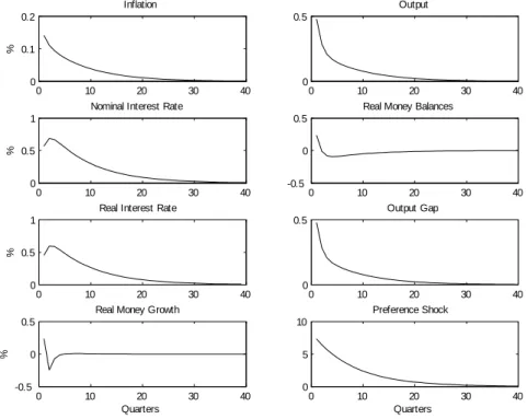
Figure 1: Preference shock

Figure 1 presents the response of key variables to a preference shock. In response to the shock, the in‡ation rate, the output, the output gap, real money balances, the nominal and the real rate of interest rise; real money growth displays a little overshooting process in the …rst periods, then returns quickly to its steady state value.

0 10 20 30 40 -0.04 -0.02 0 Inflation % 0 10 20 30 40 0 0.5 1 Output 0 10 20 30 40 -0.2 -0.1 0

Nominal Interest Rate

%

0 10 20 30 40 0

0.5 1

Real Money Balances

0 10 20 30 40 -0.2

-0.1 0

Real Interest Rate

% 0 10 20 30 40 -0.2 -0.1 0 Output Gap 0 10 20 30 40 -1 0 1

Real Money Growth

Quarters % 0 10 20 30 40 0 0.5 1 Technology Shock Quarters

Figure 2: Technology shock

In Figure 2, we plot the response of the same variables to a technology shock. The output gap, the in‡ation, the nominal and the real interest rate decrease whereas output as well as real money balances and real money growth rise.

0 10 20 30 40 0 2 4x 10 -3 _Inflation % 0 10 20 30 40 0 0.1 0.2 Output 0 10 20 30 40 0 0.01 0.02

Nominal Interest Rate

%

0 10 20 30 40 0

1 2

Real Money Balances

0 10 20 30 40 0

0.01 0.02

Real Interest Rate

% 0 10 20 30 40 0 0.005 0.01 Output Gap 0 10 20 30 40 -2 0 2

Real Money Growth

Quarters % 0 10 20 30 40 0 1 2 Money Shock Quarters

Figure 3: Money shock

Figure 3 exhibits the response to a money shock. In‡ation, the nominal and the real rate of interest, the output and the output gap rise.

0 10 20 30 40 -0.6 -0.4 -0.2 Inflation % 0 10 20 30 40 -0.4 -0.2 0 Output 0 10 20 30 40 -0.6 -0.4 -0.2

Nominal Interest Rate

%

0 10 20 30 40 -0.2

0 0.2

Real Money Balances

0 10 20 30 40 0

0.1 0.2

Real Interest Rate

% 0 10 20 30 40 -0.4 -0.2 0 Output Gap 0 10 20 30 40 -0.2 0 0.2

Real Money Growth

Quarters % 0 10 20 30 40 0.4 0.6 0.8

Interest Rate Shock

Quarters

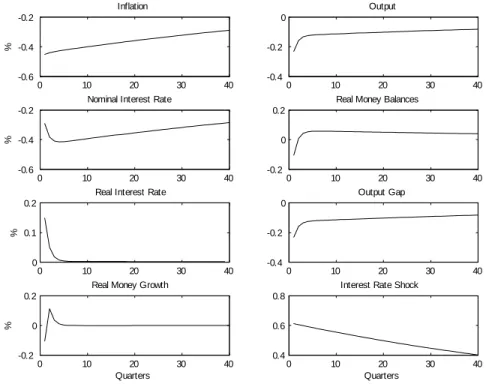
Figure 4: Interest rate shock

Figure 4 presents the response to an interest rate shock. In‡ation, the nomi-nal rate of interest, output and the output gap fall. The real rate of interest rises. A positive monetary policy shock induces a fall in interest rates due to a low enough degree of intertemporal substitution (i.e. the risk aversion parameter is high enough) which generates a large impact response of current consumption relative to future consumption. This result has been noted in, inter alia, Jeanne (1994) and Christiano et al. (1997).

0 10 20 30 40 0 0.01 0.02 Inflation % 0 10 20 30 40 -0.4 -0.2 0 Output 0 10 20 30 40 0 0.05 0.1

Nominal Interest Rate

%

0 10 20 30 40 -0.4

-0.2 0

Real Money Balances

0 10 20 30 40 0

0.05 0.1

Real Interest Rate

% 0 10 20 30 40 0 0.05 0.1 Output Gap 0 10 20 30 40 -0.5 0 0.5

Real Money Growth

Quarters % 0 10 20 30 40 0 1 2

Worked Hours Shock

Quarters

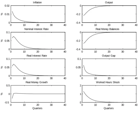
Figure 5: Labor shock

When there is a labor shock (Figure 5), in‡ation, the real and the nominal rate of interest, and the output gap increase. Output and real money balances decrease.

All these results are in line with the DSGE literature, especially with Galí (2007) and other studies on impulse response functions.

4.2

Variance decompositions

Here we analyze in two di¤erent ways the forecast error variance of each variable following exogenous shocks. The analysis is conducted …rst via an unconditional variance decomposition (Table 3), and second via a conditional variance decom-position (Figures 6 to 17).

Table 3: Unconditional variance decomposition (%)

With = 2 With = 6 "N t "Pt "it "Mt "at "Nt "Pt "it "Mt "at ^ yt 6:19 15:6 25:7 4:47 48:1 0:20 10:1 22:6 17:0 50:2 ^t 0:00 0:77 99:2 0:00 0:03 0:00 0:37 99:3 0:01 0:36 ^{t 0:21 25:5 73:3 0:03 0:98 0:14 21:1 67:7 0:26 10:8 c mp_t 1:77 0:77 1:27 83:2 13:0 0:12 0:58 0:13 76:4 22:8 ^ y_tf 11:8 0:00 0:00 5:67 82:6 0:55 0:00 0:00 16:5 82:9 c mpf_t 2:37 0:00 0:00 82:2 15:5 0:25 0:00 0:00 72:1 27:7 The unconditional variance decomposition shows that with a standard cali-bration of our model ( = 2), about half of the variance of output results from the productivity shock, about a quarter from the interest rate shock, the re-maining quarter from the other shocks. If money plays some role, this role is rather minor (an impact of less than 5%).

Yet, as Table 3 shows, the money shock contribution to the business cycle depends on the value of agents’ risk aversion. Indeed, an estimation of our model with a higher risk aversion11 ( = 6) gives interesting information as to the role of money, and more generally as to the role of each shock.

Notably, it shows that a higher coe¢ cient of relative risk aversion increases signi…cantly the role of money in a business cycle.

Figure 6: Forecast error variance decomposition of ^yt with = 2

Figure 7: Forecast error variance decomposition of ^yt with = 6

If about half of the variance of output is still explained by the productivity shock, the role of the interest rate shock and especially the role of preference and labor shocks decrease notably whereas the impact of the money shock increases from about 4% to 17%, i.e. is multiplicated by a factor of four.

The analysis through time (Figures 6 and 7) also shows that the impact of the money shock, and especially of the interest rate shock, increases a bit with the time horizon whereas it is the reverse for the preference shock.

Figure 8: Forecast error variance decomposition of ^twith = 2

Figure 9: Forecast error variance decomposition of ^twith = 6

A look at the conditional and unconditional in‡ation variance decomposition shows the overwhelming role of the interest rate shock (the monetary policy shock) which explains more than 99% of the variance. It must be noted that the change in risk aversion (when goes from 2 to 6) does not a¤ect this result, and there is no signi…cant change of the respective impacts through time (Figures 8 and 9).

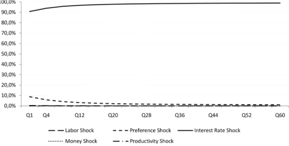
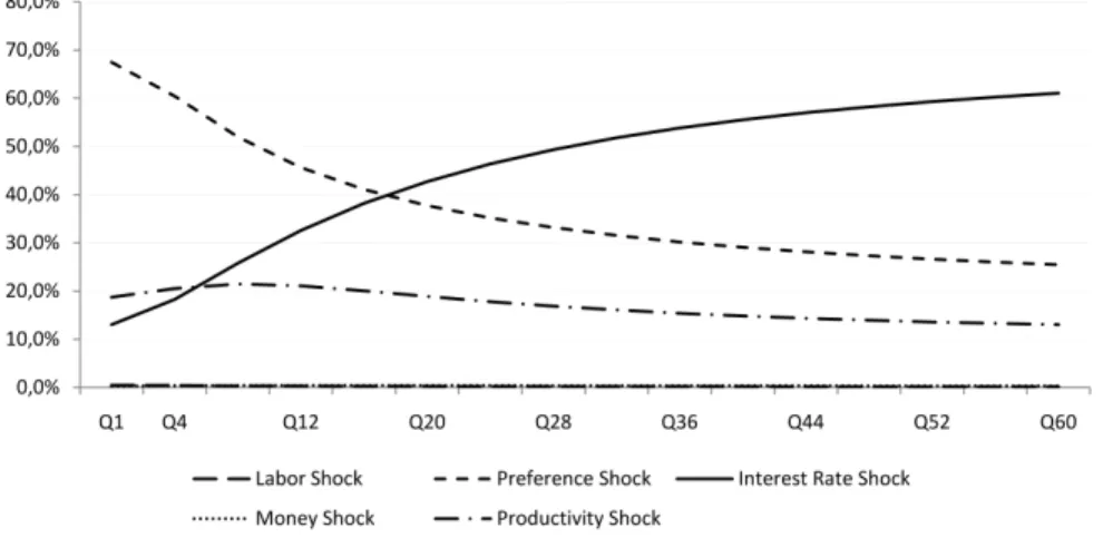
Figure 10: Forecast error variance decomposition of ^{twith = 2

Figure 11: Forecast error variance decomposition of ^{twith = 6

The interest rate variance is dominated by the direct shock on the interest rate. Yet, as risk aversion increases, the role of the productivity shock increases. The relative importance of each of these shocks changes through time (Figures 10 and 11). Over short horizons, the preference shock explains almost 70% of the nominal interest rate variance whereas the interest rate shock explains less than 20%. For longer horizons, there is an inversion: the nominal interest rate shock explains close to 70% of the variance and the preference shock a bit more than 20%.

Figure 12: Forecast error variance decomposition ofmp_ctwith = 2

Figure 13: Forecast error variance decomposition ofmp_ctwith = 6

Table 3 as well as Figures 12 and 13 show that real money balances are mainly explained by the real money balances shock and the productivity shock, with a small increase in the role of the productivity shock as risk aversion increases. The respective role of these two shocks barely changes through time.

Figure 14: Forecast error variance decomposition of ^yf_t with = 2

Figure 15: Forecast error variance decomposition of ^yf_t with = 6

It is also interesting to notice that the same type of analysis applies to the ‡exible-price output variance decomposition (Figures 14 and 15). Productivity is the main explanatory factor with a weight greater than 82%, the role of money increasing also with the relative risk aversion coe¢ cient (from a weight of about 6% to almost 17%) whereas monetary policy plays no role and labor only a minor one.

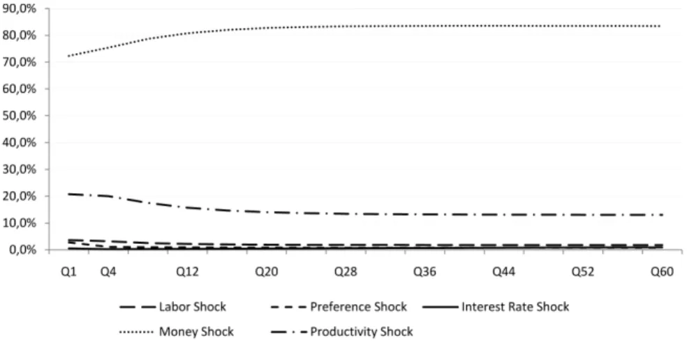
Figure 16: Forecast error variance decomposition ofmp_cf_t with = 2

Figure 17: Forecast error variance decomposition ofmp_cf_t with = 6

As Figures 16 and 17 show, the ‡exible-price real balances variance is mainly explained by the money shock, with a signi…cant impact of the productivity shock. The impact of each of these shocks does not vary much through time, but when risk aversion increases the impact of the productivity shock also increases.

5

Conclusion

In this paper, we built and empirically tested a model of the Euro zone, with a special emphasis on the role of money. The model follows the New Keynesian DSGE framework, but with money in the utility function whereby real money balances a¤ect the marginal utility of consumption. By using bayesian estima-tion techniques, we shed light on the determinants of output and in‡aestima-tion, but also of interest rate, real money balances, ‡exible-price output and ‡exible-price real money balances variances. On that respect we further investigate the role of money, especially when intertemporal risk aversion changes.

Half of the variance of output is explained by the productivity shock, the other half by a combination of labor, preference, interest rate and money shocks. Almost the totality of the in‡ation variance is a consequence of the interest rate shock. The interest rate variance depends mainly on the interest rate shock, but the preference shock is also signi…cant, as well as, to a lesser extent, the productivity shock. Real balances react essentially to money shocks, with a signi…cant role left to the productivity shock. Interestingly, the ‡exible-price output variability depends strongly on the productivity shock, but the money shock remains signi…cant. The ‡exible-price real balances variance is mainly explained by the money shock, with a signi…cant impact of the productivity shock. These results are sensible and rather in line with prior expectations. We believe that this corroborates the credibility of our model.

To investigate further the role of each shock, especially the money shock, we calibrated the model with di¤erent risk aversion coe¢ cients.

The …rst calibration of the model with a standard risk aversion shows that money plays a minor role in explaining output variability, a result in line with current literature (Andrès et al., 2006; Ireland, 2004). Other calibrations with higher risk aversion imply that money plays a non-negligible role in explaining output ‡uctuations. And the more agents are risk averse, the higher the impact of money on output. This result di¤ers from existing literature using New Keynesian DSGE frameworks with money, neglecting the role of a high enough risk factor.

On the other hand, the explicit money variable does not appear to have a notable direct role in explaining in‡ation variability, the overwhelming explana-tory factor being the interest rate (monetary policy) whatever the level of risk aversion.

If these results are trustworthy, it can be inferred that the last …nancial crisis, by changing economic agents’ perception of risks, may have increased the role of real money balances in the transmission mechanisms and in output changes.

6

Appendix

6.1

Aggregate consumption and price index

Let Ct= R₀1Ct(i)1

1 "_di

" " 1

be a consumption index where Ct(i) represents

the quantity of good i consumed by the household in period t. This requires that Ctbe maximized for any given level of expendituresR₀1Pt(i) Ct(i) di where

Pt(i) is the price of good i at time t. The maximization of Ct for any given

expenditure level R₀1Pt(i) Ct(i) di = Zt can be formalized by means of the

Lagrangian L = Z 1 0 Ct(i)1 1 "_di " " 1 Z 1 0 Pt(i) Ct(i) di Zt (33)

The associated …rst-order conditions are Ct(i)

1 "_C

1

t = Pt(i) for all i 2

[0; 1]. Thus, for any two goods (i; j), Ct(i) = Ct(j)

Pt(i)

Pt(j) "

(34) which can be substituted into the expression for consumption expenditures to yield Ct(i) = P_Pt(i)_t

" Zt

Pt for all i 2 [0; 1] where Pt =

R1 0 Pt(i) 1 " di 1 1 " is an aggregate price index. The latter condition can then be substituted into the de…nition of Ctto obtain

Z 1 0

Pt(i) Ct(i) di = PtCt (35)

Combining the two previous equations yields the demand schedule equation Ct(i) = P_Pt(i)_t

"

Ctfor all i 2 [0; 1].

6.2

Optimization problem

Our Lagrangian is given by Lt= Et "₁ X k=0 k Ut+k t+kVt+k # (36) where Vt= Ct+ Mt Pt + Qt Bt Pt Bt 1 Pt Wt Pt Nt Mt 1 Pt (37) and Ut= e" P t 1 1 X 1 t e"Nt _N1+ t 1 + ! (38)

where Xt = (1 b) Ct1 + be"

M

t Mt

Pt

1 11

is the non-separable part of the utility function.

The …rst order condition related to consumption expenditures is given by

t= e"

P

t _{(1 b) C}

t Xt (39)

where t is the Lagrange multiplier associated with the budget constraint at

time t.

The …rst order condition corresponding to the demand for contingent bonds implies that Qt= Et t+1 t Pt Pt+1 (40) The demand for cash that follows from the household’s optimization problem is given by be"Mt _e"Pt Mt Pt X_t = t Et t+1 Pt Pt+1 (41) which can be naturally interpreted as a demand for real balances. The latter is increasing in consumption and inversely related to the nominal interest rate, as in conventional speci…cations. e"Pt _e"Nt _N t = t Wt Pt (42)

6.3

Log linearization

Log linearizing the Lagrangian multiplier (39) around its steady state yields ^_{t= "}P t ^ct+ ( ) a1^ct+ (1 a1) m^t p^t+ 1 1 " M t (43) where a1 = (1 b)C 1 (1 b)C1 _+b(M P)

1 is a constant term where C and

M

P are

respec-tively consumption and real money balances at the steady state12_{. We obtain}

from (39), (40) and (41) the following expression for a1

a1=

1 1 + _{1 b}b

1

(1 ) 1

Log linearizing (40) around its steady state yields (with Qt= e it)

^{t= Et " "P t+1+ (a1( ) ) ^ct+1 + (1 a1) ( ) m^t+1 p^t+1+₁1 "Mt+1 ^t+1 # (44)

1 2_{In order to determine (43), (44) and (46), we need to log linearize X}

t around its steady state: ^Xt= a1^ct+ (1 a1) ₁1 ^"Mt + ( ^mt p^t)

Log linearizing (41) around its steady state and up to an uninteresting con-stant yields

"M_t ( ^mt p^t) + ^ct= a2^{t (45)

where a2 is such as \1 Qt = a2^{t i.e. a2 = _exp(11_{) 1} because 1 is the steady

state interest rate.

Equation (45) is the intertemporal optimality condition setting the marginal rate of substitution between money and consumption equal to the opportunity cost of holding money.

Log linearizing (42) around its steady state yields ^ nt (a1( ) ) ^ct ( ) (1 a1) m^t p^t+ 1 1 " M t + "Nt = ^wt p^t (46) Equation (46) is the condition for the optimal consumption-leisure arbitrage, implying that the marginal rate of substitution between consumption and labor is equated to the real wage.

6.4

Calibration and results (

= 6)

Table 4: Calibration and estimation of structural parameters13

Law Prior Posterior Posterior Standard Con…dence

mean deviation mean deviation interval

beta 0:99 0:005 0:9922 0:0030 [0:9860; 0:9985] normal 6:0 0:05 5:9906 0:0500 [5:9105; 6:0723] normal 1:2 0:05 1:4075 0:0357 [1:3493; 1:4678] normal 1:0 0:05 1:0100 0:0498 [0:9322; 1:0996] beta 0:66 0:05 0:8224 0:0232 [0:7807; 0:8602] " normal 6:0 0:05 6:0024 0:0500 [5:9211; 6:0829] beta 0:33 0:05 0:4700 0:0583 [0:3794; 0:5631] b beta 0:4 0:05 0:3984 0:0508 [0:3180; 0:4752] i beta 0:6 0:05 0:5781 0:0358 [0:5203; 0:6378] normal 3:5 0:05 3:5038 0:0499 [3:4128; 3:5846] x normal 1:5 0:05 1:5280 0:0493 [1:4479; 1:6089] a beta 0:8 0:075 0:9006 0:0248 [0:8641; 0:9425] i beta 0:8 0:075 0:9882 0:0042 [0:9812; 0:9957] p beta 0:8 0:075 0:8251 0:0255 [0:7849; 0:8667] m beta 0:8 0:075 0:9352 0:0179 [0:9047; 0:9639] n beta 0:8 0:075 0:7987 0:0759 [0:6862; 0:9152] a invgamma 1 1 2:1607 0:2511 [1:7459; 2:5606] i invgamma 1 1 0:5743 0:0675 [0:4415; 0:6864] p invgamma 5 1 7:7275 0:7471 [6:4409; 8:9630] m invgamma 1 1 1:4870 0:1059 [1:3021; 1:6521] n invgamma 1 1 0:9438 0:2150 [0:3243; 1:6599]

Results are based on 10 chains, each with 100000 draws based on the Metropolis algorithm.

6.5

Priors and posteriors (

= 2)

0 2 4 0 1 2 3 σ_a 0 2 4 0 0.5 1 1.5 σ_n 1 2 3 4 0 2 4 6 σ_i 4 6 8 10 12 0 0.2 0.4 σ_p 1 2 3 4 0 2 4 σ_m 0.2 0.4 0.6 0 2 4 6 8 α 0.97 0.98 0.99 1 0 50 100 β 0.5 0.6 0.7 0.8 0.9 0 5 10 θ 1.2 1.4 1.6 0 5 10 ν 1.8 2 2.2 0 2 4 6 8 σ 0.2 0.4 0.6 0 2 4 6 8 b 0.8 1 1.2 0 2 4 6 8 η 5.8 6 6.2 0 2 4 6 8 ε 0.4 0.5 0.6 0.7 0 5 10 λ i 3.2 3.4 3.6 3.8 0 2 4 6 8 λ_π 1.4 1.6 1.8 0 2 4 6 8 λ y 0.6 0.8 1 0 5 10 ρ a 0.4 0.6 0.8 1 0 2 4 ρ n 0.6 0.7 0.8 0.9 0 10 20 ρ_p 0.6 0.8 1 0 50 100 ρ_i 0.6 0.8 1 0 10 20 ρ_m P ri or P os terior Mean

The vertical line denotes the posterior mode, the grey line is the prior dis-tribution, and the black line is the posterior distribution.

6.6

Priors and posteriors (

= 6)

1 2 3 4 0 0.5 1 1.5 σ a 0 2 4 0 0.5 1 1.5 σ n 1 2 3 4 0 2 4 6 σ_i 4 6 8 10 12 0 0.2 0.4 σ_p 1 2 3 4 0 2 4 σ_m 0.2 0.4 0.6 0 2 4 6 8 α 0.97 0.98 0.99 1 0 50 100 β 0.5 0.6 0.7 0.8 0.9 0 5 10 15 θ 1.1 1.2 1.3 1.4 1.5 0 5 10 ν 5.8 6 6.2 0 2 4 6 8 σ 0.2 0.4 0.6 0 2 4 6 8 b 0.8 1 1.2 0 2 4 6 8 η 5.8 6 6.2 0 2 4 6 8 ε 0.4 0.5 0.6 0.7 0 5 10 λ i 3.4 3.6 3.8 0 2 4 6 8 λ_π 1.4 1.6 1.8 0 2 4 6 8 λ_y 0.6 0.8 1 0 5 10 15 ρ a 0.4 0.6 0.8 1 0 2 4 ρ n 0.6 0.7 0.8 0.9 0 5 10 15 ρ_p 0.6 0.8 1 0 20 40 60 80 ρ_i 0.6 0.8 1 0 10 20 ρ_m P ri or P os terior Mean

6.7

Static analysis

The following table highlights the derivatives of the macro-coe¢ cients with re-spect to , knowing that a1 and a2are independent of , = 1:2, and 2.

@ @ y a a1(1 )(1+ ) (( ( )a1)(1 )+ + )2 < 0 y m (1 )(1 a1)( + + (1 )) (( ( )a1)(1 )+ + )2 < 0 y c a1log(""1)(1 ) 2 (( ( )a1)(1 )+ + )2 < 0 y sm 11 (1 )(1 a1)( + + (1 )) (( ( )a1)(1 )+ + )2 > 0 y sn a1(1 )2 (( ( )a1)(1 )+ + )2 > 0 m y a1a2 > 0 m y+1 a1a2 < 0 x a1(1₁ )(1_{+ "} )1 > 0 m (1 )(1 a_{1 + "}1)(1 )1 > 0 r _{( a}a1 1( ))2 < 0 mp _{( a}(1 a1) 1( ))2 > 0 sp _{( a1}a₍1 ₎₎2 > 0 sm _{( a}1 a1 1( ))21 < 0 i 0

References

[1] Adolfson, Malin, Stefan Laseen, Jesper Linde and Mattias Villani. (2007). ’Bayesian estimation of an open economy DSGE model with incomplete pass-through.’Journal of International Economics, vol. 72(2), pp. 481-511. [2] Assenlacher-Wesche, Katrin and Stefan Gerlach. (2006). ’Understanding the link between money growth and in‡ation in the Euro area.’ CEPR Discussion Paper No. 5683.

[3] Andrés, Javier, J. David López-Salido and Edward Nelson. (2009). ’Money and the natural rate of interest: Structural estimates for the United States and the euro area.’Journal of Economic Dynamics and Control, vol. 33(3), pp. 758-776.

[4] Andrés, Javier, J. David López-Salido, and Javier Vallés. (2006). ’Money in an Estimated Business Cycle Model of the Euro Area.’ The Economic Journal, vol. 116(511), pp. 457-477.

[5] Bhattacharjee, Arnab and Christoph Thoenissen. (2007). ’Money and Mon-etary Policy in Dynamic Stochastic General Equilibrium Models.’ The Manchester School, vol. 75(S1), pp. 88-122.

[6] Berger, Hlege and Pär Österholm. (2008). ’Does money growth Granger-cause in‡ation in the Euro Area ? Evidence from out-of-sample forecasts using Bayesian VARs.’IMF Working Paper No. 53.

[7] Brunner, Karl, and Allan H. Meltzer (1968). ’Liquidity Traps for Money, Bank Credit and Interest Rates.’Journal of Political Economy, vol. 76, pp. 1-37.

[8] Casares, MigueI. (2007). ’Monetary Policy Rules in a New Keynesian Euro Area Model.’ Journal of Money, Credit and Banking, vol. 39(4), pp. 875-900.

[9] Christiano, Lawrence, Roberto Motto and Massimo Rostagno. (2007). ’Two reasons why money and credit may be useful in monetary policy.’ NBER Working Paper No. 13502.

[10] Clarida, Richard, Jordi Galí and Mark Gertler. (1999). ’The science of monetary policy: a new Keynesian perspective.’Journal of Economic Lit-erature, vol. 37(4), pp. 1661-1707.

[11] Dixit, Avinash K. and Joseph E. Stiglitz. (1977). ’Monopolistic Compe-tition and Optimum Product Diversity.’American Economic Review, vol. 67(3), pp. 297-308.

[12] Fagan, Gabriel, Jérôme Henry and Ricardo Mestre. (2001). ’An area-wide model (AWM) for the euro area.’European Central Bank, Working Paper No. 42.

[13] Fourçans, André and Radu Vranceanu. (2006). ’The ECB monetary policy: Choices and challenges.’ Journal of Policy Modelling, vol. 29(2), pp. 181-194.

[14] Friedman, Milton. (1956). ’The Quantity Theory of Money: A Restate-ment.’Studies in the Quantity Theory of Money, IL.: University of Chicago Press.

[15] Galí, Jordi and Mark Gertler. (2007). ’Macroeconomic modelling for mon-etary policy evaluation.’Journal of Economic Perspectives, vol. 21(4), pp. 25-45.

[16] Galí, Jordi. (2008). Monetary Policy, In‡ation and the Business Cycle: An Introduction to the New Keynesian Framework. Princeton, NJ.: Princeton University Press.

[17] Garcia-Iglesias, Jesus M. (2007). ’How the European Central Bank decided its early monetary policy ?.’Applied Economics, vol. 39(7), pp. 927-936. [18] Gerlach, Stefan. (2004). ’The Two Pillars of the European Central Bank.’

[19] Golinelli, Roberto and Sergio Pastorello. (2002). ’Modelling the demand for M3 in the Euro area.’The European Journal of Finance, vol. 8(4), 371-401. [20] Hofmann, Boris. (2008). ’Do monetary indicators lead Euro area in‡ation

?.’European Central Bank, Working Paper No. 867.

[21] Ireland, Peter N. (2004). ’Money’s Role in the Monetary Business Cycle.’ Journal of Money, Credit and Banking, vol. 36(6), pp. 969-983.

[22] Jones, Barry E. and Livio Stracca. (2008). ’Does Money Matter In The Is Curve? The Case Of The UK.’ The Manchester School, vol. 76(S1), pp. 58-84.

[23] Kremer, Jana, Giovanni Lombardo and Thomas Werner. (2003). ’Money in a New-Keynesian model estimated with German data.’Deutsche Bundes-bank, Working Paper No. 15.

[24] Kaufmann, Sylvia and Peter Kugler. (2008). ’Does Money Matter for In-‡ation in the Euro Area ?.’Contemporary Economic Policy, vol. 26(4), pp. 590-606.

[25] Leeper, Eric and Jennifer Roush. (2003). ’Putting “M” back in monetary policy.’Journal of Money, Credit and Banking, vol. 35(6), pp. 1217-1256. [26] Lindé, Jesper. (2005). ’Estimating New-Keynesian Phillips curves: A full

information maximum likelihood approach.’ Journal of Monetary Eco-nomics, vol. 52(6), pp. 1135-1149.

[27] Meltzer, Allan H. (1995). ’Monetary, Credit, and (other) Transmission Processes.’Journal of Economic Perspectives, vol. 9(4), pp. 49-73.

[28] Meltzer, Allan H. (1999). ’The Transmission Process.’mimeo, March. [29] Nelson, Edward. (2008). ’Why money growth determines in‡ation in the

long run: Answering the Woodford critique.’Journal of Money, Credit and Banking, vol. 40(8), pp. 1791-1814.

[30] Nelson, Edward. (2002). ’Direct e¤ects of base money on aggregate demand: theory and evidence.’Journal of Monetary Economics, vol. 49(4), pp. 687-708.

[31] Neumann, Manfred J.M. and Claus Greiber. (2004). ’In‡ation and core money growth in the Euro Area.’Deutsche Bundesbank, Discussion Paper No. 36.

[32] Reynard, Samuel. (2007). ’Maintaining low in‡ation: Money, interest rates, and policy stance.’ Journal of Monetary Economics, vol. 54(5), pp. 1441-1471.

[33] Smets, Frank and Raf Wouters. (2003). ’An Estimated Dynamic Stochastic General Equilibrium Model for the Euro Area.’ Journal of the European Economic Association, vol. 1(5), pp. 1123-175.

[34] Stark, Jürgen. (2006). ’The role of money: Money and monetary policy in the twenty-…rst century.’Fourth ECB Central Banking Conference, Frank-furt am Main.

[35] Surico, Paolo. (2007). ’The monetary policy of the European Central Bank.’ Scandinavian Journal of Economics, vol. 109(1), pp. 115-135.

[36] Söderström, Ulf. (2005). ’Targeting In‡ation with a Role for Money.’Eco-nomica, vol. 72(288), pp. 577-596.

[37] Walsh, Carl E. (1998). Monetary Theory and Policy. Cambridge, MA.: The MIT Press.

[38] Woodford, Michael. (2003). Interest and prices: Foundations of a theory of monetary policy. Princeton, NJ.: Princeton University Press.