Transport and modeling of stratospheric inorganic chlorine

(1)

HAL Id: hal-00302888

https://hal.archives-ouvertes.fr/hal-00302888

Submitted on 21 Jun 2007

HAL is a multi-disciplinary open access

archive for the deposit and dissemination of sci-entific research documents, whether they are pub-lished or not. The documents may come from teaching and research institutions in France or abroad, or from public or private research centers.

L’archive ouverte pluridisciplinaire HAL, est destinée au dépôt et à la diffusion de documents scientifiques de niveau recherche, publiés ou non, émanant des établissements d’enseignement et de recherche français ou étrangers, des laboratoires publics ou privés.

Transport and modeling of stratospheric inorganic

chlorine

D. W. Waugh, S. E. Strahan, P. A. Newman

To cite this version:

D. W. Waugh, S. E. Strahan, P. A. Newman. Transport and modeling of stratospheric inorganic chlorine. Atmospheric Chemistry and Physics Discussions, European Geosciences Union, 2007, 7 (3), pp.8597-8616. �hal-00302888�

(2)

ACPD

7, 8597–8616, 2007 Transport and modeling of Cl_y D. W. Waugh et al. Title Page Abstract Introduction Conclusions References Tables Figures ◭ ◮ ◭ ◮ Back Close

Full Screen / Esc

Printer-friendly Version Interactive Discussion

EGU Atmos. Chem. Phys. Discuss., 7, 8597–8616, 2007

www.atmos-chem-phys-discuss.net/7/8597/2007/ © Author(s) 2007. This work is licensed

under a Creative Commons License.

Atmospheric Chemistry and Physics Discussions

Transport and modeling of stratospheric

inorganic chlorine

D. W. Waugh1, S. E. Strahan2, and P. A. Newman3

1

Department of Earth and Planetary Science, Johns Hopkins University, MD, USA

2

University of Maryland Baltimore County, Goddard Earth Sciences and Technology Center, MD, USA

3

NASA Goddard Space Flight Center, Greenbelt, MD, USA

Received: 23 May 2007 – Accepted: 8 June 2007 – Published: 21 June 2007 Correspondence to: D. W. Waugh ([email protected])

(3)

ACPD

Full Screen / Esc

EGU

Abstract

Correctly modeling stratospheric inorganic chlorine (Cly) is crucial for modeling the

past and future evolution of stratospheric ozone. However, comparisons of the chem-istry climate models used in the latest international assessment of stratospheric ozone depletion have shown large differences in the modeled Cly, with these differences

ex-5

plaining differences in the simulated evolution of ozone over the next century. Here in, we examine the role of transport in determining the simulated Cl_y using three simula-tions from the same off-line chemical transport model that have the same lower tro-pospheric boundary conditions and the same chemical solver, but differing resolution and/or meteorological fields. These simulations show that transport plays a key role in

10

determining the Cl_ydistribution, and that Cl_ydepends on both the time scales and path-ways of transport. The time air spends in the stratosphere (e.g., the mean age) is an important transport factor determining stratospheric Cly, but the relationship between

mean age and Cl_y is not simple. Lower stratospheric Cl_y depends on the fraction of air that has been in the upper stratosphere, and transport differences between models

15

having the same mean age can result in differences in the fraction of organic chlorine converted into Cl_y. Differences in transport pathways result in differences in vertical profiles of CFCs, and comparisons of observed and modeled CFC profiles provides a stringent test of transport pathways in models.

1 Introduction

20

The observed changes in ozone over the last two decades, as well as the expected fu-ture increases, are primarily the result of changes in the concentration of stratospheric inorganic chlorine (Cl_y) and bromine (Br_y). Therefore, correctly modeling stratospheric Cly and Bry is crucial for modeling past and future stratospheric ozone levels.

How-ever, comparisons of the coupled chemistry climate models (CCMs) used in the latest

25

(4)

dif-ACPD

Full Screen / Esc

EGU ferences in the modeled Cl_y, both in terms of magnitude and the date that Cl_y returns

to pre-1980 values (Eyring et at.,2006, 20071). Furthermore, these differences appear to explain the differences in simulated ozone between the models, e.g. models with a later return of Clyto pre-1980 values also have later return of ozone. Given its

impor-tance for modeling ozone and the large differences between models, it is important to

5

understand the causes of the differences in the simulations of Cly.

In the above CCM simulations the same time series of organic chlorine species (e.g., chlorofluorocarbons, CFCs) are specified in the lower troposphere and the same, or very similar, radiation schemes and chemical reactions are included in the models. This indicates that the differences in Cly are not due to differences in source gases,

10

radiation, or stratospheric chemistry but are most likely due to differences in transport. Here we explore this issue further by examining Cl_y from three simulations from the same off-line chemical transport model (CTM). The simulations use the same lower tro-pospheric concentration boundary conditions and the same chemical solver, but differ-ing resolution and/or meteorological fields. As the boundary conditions and chemistry

15

are exactly the same any differences in Clyare due to differences in the transport.

The model and simulations are described in the next section. In Sect. 3 we compare the Cl_y and mean age Γ from the CTM simulations, and also compare the simulated Cly with an estimate using the formulation used byNewman et at.(2006) to calculate

EESC. These comparisons show that transport plays a key role in determining the

20

distribution of Cl_y, and that Cl_y depends on both the time scales and pathways of transport.

1

Eyring, V., Waugh, D. W., Bodeker, G. E., et al.: Multi-model projections of stratospheric ozone in the 21st century, J. Geophys. Res., 112, to appear, 2007.

(5)

ACPD

Full Screen / Esc

EGU

2 Model description

The simulations examined are performed using the NASA Global Modeling Initiative (GMI) CTM (Douglass et at.,2004 and references therein). The CTM includes a full description of stratospheric chemistry, and can be driven by meteorological data from either a free-running general circulation model (GCM) or from a data assimilation

sys-5

tem (DAS). We consider both cases here: Simulations are analyzed that used either the Goddard Earth Observing System (GEOS) DAS (Schubert et at.,1993) or the GEOS-4 GCM (Bloom et al.,2005).

As well as differing meteorological fields, the horizontal resolution and top of the CTM differs between some of the simulations. We consider three simulations:

10

1. GCM winds, 2◦

latitude × 2.5◦ _{longitude, top at 0.015 hPa with 33 levels}

(“GCM-HIGH”). 2. GCM winds, 4◦

latitude × 5◦_{longitude, top at 0.4 hPa with 28 levels (“GCM-LOW”).}

3. DAS winds, 4◦

latitude × 5◦_{longitude, top at 0.4 hPa with 28 levels (“DAS-LOW”).}

The two “LOW” simulations are described inConsidine et al.(2004), while the

GCM-15

HIGH simulation is described inDouglass et at.(2006).

All three simulations use the same chemical solver (seeDouglass et at.,2004) and the concentration of halogens in the lower troposphere are specified as in table 4B-2 of WMO(2003). In each case a single year of meteorological fields is used in the CTM, but the source gas boundary conditions vary between years. In the GCM-HIGH

simu-20

lation the boundary conditions start in 1974 and end in 2025. The “LOW” simulations were spun up for 5 years at 1995 source gas boundary conditions and then integrated through the year 2030. (Because 1995 boundary conditions were used rather than 1990 to 1994 conditions in the spin up of the “LOW” simulations the stratospheric chlo-rine is over-estimated in the early part of these simulations. However, the difference

25

is much smaller than the inter-model differences discussed below.) For all simulations fields have been archived every 5 years.

(6)

ACPD

Full Screen / Esc

EGU Additional twenty year simulations of an age spectrum tracer (i.e. the mixing ratio of

a conserved tracer was set to 1 for the first month and then set to 0 for the rest of the run, in the lowest two model levels) were also run. This tracer allows calculation of the mean age of air in the stratosphere as well as the full age spectra (Waugh and Hall, 2002).

5

3 Results

3.1 CTM simulations

We first consider the Cly distribution in the three simulations. As shown in Fig. 1(a–

c; top panels) the general features of the Cl_y distributions are the same, e.g., there are values larger than 3 ppb in the upper stratosphere and lower values in the tropics

10

than mid- and high latitudes. However, there are quantitative differences, especially in the wintertime (southern) polar regions. For example, the South Pole Cl_y at 20 km varies from less than 1.5 ppb to around 3 ppb. As the surface concentrations and the chemistry are the same in all three simulations, this confirms the CCM results (Eyring et at.,2006) that transport plays a key role in determining Cly.

15

As Cl_y is formed by conversion of organic chlorine into inorganic chlorine species within the stratosphere, the time spent in the stratosphere is expected to play an im-portant role in determining Cly. We therefore next consider the distributions of the

mean age Γ. (Γ is calculated from simulations of the age spectra, and represents the annual-mean Γ, seeWaugh and Hall,2002.) As shown in Fig.1(d–f; bottom panels)

20

the mean age differs among all three simulations. The largest differences are between DAS-LOW and the two GCM simulations, with much younger ages in DAS-LOW. There are also differences in age between GCM-LOW and GCM-HIGH, but these are small in the lower stratosphere (e.g., the South Pole mean age at 20km is around 4.7 yrs in both GCM simulations).

25

Comparison of the Cly and Γ distributions shows that Cly is, in general, larger for

(7)

ACPD

Full Screen / Esc

EGU older Γ. However, this comparison also suggests that differences in Γ do not explain all

the differences in Cly. This is clearly seen in vertical profiles within the spring Antarctic

vortex: Around 20 km Γ from the two GCM based simulations are the same but there is a large difference in Cly, see Fig.2a, b. Conversely, above this altitude there are much

larger differences in mean age than in Clybetween these two simulations. Hence, there

5

is not a simple relationship between differences in mean age and those in Cly.

To explore the differences in Cly in more detail we compare the time series of lower

stratospheric Cl_yat two locations where Γ is similar in the two GCM based simulations, see Fig. 3. In mid-latitudes the two GCM simulations have very similar Cly (Fig.3a),

but at the polar location there is a large difference (Fig.3b). At both locations Γ and

10

Cl_yfrom the DAS simulation are smaller than from the GCM simulations.

The differences in Cly could be due to differences in the simulated total amount of

chlorine Cltot(the sum of organic and inorganic chlorine) in the stratosphere. However,

Cl_tot is very similar among all three simulations (dashed curves in Fig.3). There is a slight time shift between the DAS and two GCM simulations, which is consistent with

15

the approximately 2 year difference in the mean age. However, the magnitude of Cltotis

very similar and differences in Cltotdo not explain the differences in Cly. As well as the

time shift in Cltotbetween the DAS and GCM simulations there are slight differences in

the peak values, which are due to differences in the width of the age spectra. However these differences are insignificant compared to the differences in Cly.

20

The above shows that the time spent in the stratosphere is important but this is not the sole transport factor determining stratospheric Cly(and differences between

the simulations). Hence, the paths taken to get to a particular location must also be important for determining Cly.

3.2 Theory

25

To understand the differences in simulated Clywe estimate the Clyusing the formulation

(8)

ACPD

Full Screen / Esc

EGU contribution from each CFC, i.e.,

Cl∗ y(t)=

X

i

n_iF_iρˆ_i(t) (1)

wheren_i is the number of chlorine atoms in source gas i, ˆρ_i is the source gas mix-ing ratio if the gas was conserved in the stratosphere, and F_i the fraction of species dissociated while it has been in the stratosphere. The mixing ratio ˆρi depends on the

5

tropospheric concentrations (ρi ,trop) and the troposphere to stratosphere transport time

scales: ˆ ρi(t)= Zt −∞ ρi,trop(t′)G(t − t′)d t′. (2)

whereG(t) is the age spectrum. The fractional release is given by

F_i=( ˆρ_i− ρi)/ ˆρi, (3)

10

whereρ_i is the actual concentration of the source gas at given stratospheric location. We focus here on lower stratospheric Cl_y and, as inNewman et at.(2006), assume that the fractional releases are solely a function of the mean age, i.e. Fi=Fi(Γ).

Al-though we assume a dependence only on the mean age it is important to know that the release rates also depend on pathways, and the functional relationships are not

15

necessarily the same for all simulations. Fi(Γ) are determined separately for the three

simulations using the method ofSchauffler et al.(2003) applied to the simulated fields for 2000.

We first compare Cl∗

y with the directly simulated Cly. In these calculations of Cl∗y we

use the age spectrum G(t) simulated within the CTMs (see Sect. 2), theρ_i,tropused in

20

the CTMs, and the above estimates ofF_i. As shown in Fig.4the Cl∗

yestimated from G(t)

andF matches the time evolution of Cly and the differences between the simulations.

There are some differences between Cl∗

y and Clyfor GCM-LOW, but these differences

are much smaller than model-model differences, and Cl∗

y is a good representation of

Cl_y at a few % level. (Note virtually the same Cl∗

y is obtained if the approximate age

25

(9)

ACPD

Full Screen / Esc

EGU spectrum used by Newman et al. (2006), an inverse Gaussian age spectra with width

equal to half the mean age, is used rather than the true model age spectrum, see dashed curves in Fig.4.)

Given this general agreement we can now explore the differences in the individual contributions to Cl∗

y. Asρi ,tropis the same in all simulations and the differences in Cltot

5

are small, differences in fractional release are the main cause for differences in Cly.

Fig.5shows the variation of lower stratospheric concentration (a, b; top panels) and fractional releaseF (c, d; bottom panels) with mean age Γ, for 11 (left) and

CFC-12 (right). Very similar results are found for other CFCs. Focusing first on the two GCM based simulations we see that the CFC concentrations andF are very similar for Γ<4

10

years, but differences occur for older ages. For old ages (polar air) the CFC concen-trations are lower for GCM-HIGH, which means that the fraction of CFC converted into Clyis larger (i.e. F is larger). Thus, differences in transport can result in differences in

the fraction of organic chlorine converted into Cl_y, and hence differences in Cly, for air

with the same mean age.

15

The fractional release rates for the DAS simulation differs from both the GCM simu-lations. The maximum values of both Γ and F are smaller in the DAS simulation (the smallerF is consistent with the smaller lower stratospheric Cly in the DAS simulation).

For fixed Γ, F is larger from the DAS simulation than the GCM simulations. This is because comparing air with the same Γ in the DAS and a GCM simulation is not a

20

comparison of air at the same location. A lower stratospheric location in DAS with the same Γ as in one of the GCM simulations will be at a higher latitude, e.g., air at 20 km with Γ=2.4 yrs in the DAS simulation is at the South Pole, whereas Γ=2.4 yrs is in the subtropics in both GCM simulations (Fig. 1). A higher latitude location generally has a higher percentage of air that has been in CFC loss regions, and so higher latitude

25

air with the same age will have higherF . If comparisons between F are made at the

same location thenF is smaller in the DAS simulation than the GCM simulations, and

(10)

ACPD

Full Screen / Esc

EGU The differences in the fractional release of CFCs in the Antarctic vortex can be clearly

seen in the vertical profiles of the CFCs, see Fig.2c, d. One consequence of this is that observations of CFCs can probably be used to differentiate model simulations of Cl_y. For example, the solid circles in Fig.2c, d show the monthly average CFCs near 80◦_{S from the Atmospheric Chemistry Experiment (ACE) (Bernath et al.,} ₂₀₀₅₎

ob-5

servations in September 2005. (The model and ACE CFCs are from September rather than October as ACE samples south of 79◦_{S in early September but not later.) All three}

simulations overestimate the observed CFC abundances, with the best agreement for the GCM-HIGH simulation. This suggests that GCM-HIGH has the most realistic sim-ulation of Cl_y.

10

Unfortunately, the corresponding profiles of Cl_y cannot be determined directly from ACE as Cl2O2(which is a significant reservoir of Clyinside Antarctic lower stratospheric

vortex in September) is not measured. However, measurements of HCl and ClO in October 2005 by Aura MLS indicate that at 20 km Cl_y is around 3.3 ppb (Figs. 4–8 of WMO,2007). Consistent with the above CFC comparisons, the modeled Cly are too

15

low, with GCM-HIGH the most realistic.

4 Discussion

Previous analysis of models has shown that Γ is very important for correctly estimating Cl_y. However, the above comparisons have shown that although the mean age in the polar lower stratosphere may be the same in two simulations, this does not mean

20

that Cly will be the same. It is important to consider the pathways that the air has

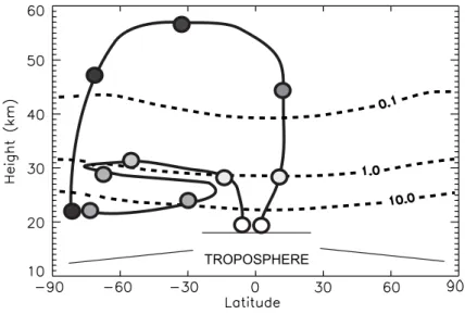
taken, which can be different even if Γ is the same. Even if two parcels have the same Γ one parcel could have lower CFC concentrations, higher fractional releases, and larger Cly if this parcel spent more time in regions with larger CFC photolysis. This

is illustrated schematically in Fig. 6 which shows two parcels with same transit time

25

from the tropopause but different pathways. As a result the two parcels have different photochemical exposure (Schoeberl et at.,2000) and Cly.

(11)

ACPD

Full Screen / Esc

EGU The larger CFC concentrations, and hence smaller Cl_y, in the GCM-LOW simulation

could be explained by a smaller fraction of the polar air having been in the middle-upper stratosphere where CFCs are photolyzed. This is supported by the analysis of Strahan and Polansky (2006). They showed that with lower horizontal resolution there are leakier transport barriers (in subtropics and edges of polar vortices), which results

5

in more rapid transport of young air to polar regions. The leakier barriers also allow more recirculation of air between the tropics and extratropics, allowing air to becomes old without spending time in the upper stratosphere. The greater influence of young air in the GCM-LOW simulation can also be seen in the age spectra, see Fig.7(see also Fig. 14 ofStrahan and Polansky , 2006). In the GCM-LOW simulation there is

10

a much higher percentage of young air (<2 years) than in the GCM-HIGH simulation.

Also, air arrives continuously in GCM-LOW whereas the GCM-HIGH simulation shows an episodic annual injection of air into the polar region in the transport (Strahan and Polansky ,2006).

5 Conclusions

15

The CTM simulations presented here show that transport plays a key role in determin-ing the distribution of Cly, and that large differences in Cly can occur in models using

the same surface concentrations of source gases and same chemistry. The time air spends in the stratosphere (e.g., the mean age, Γ) is an important factor but this is not the sole transport factor determining stratospheric Cly. Stratospheric Clyalso depends

20

on where the air has been. Differences in transport pathways can result in differences in the fraction of air that has been in the upper stratosphere, where organic chlorine is converted into Cl_y, even for air with the same mean age. Thus there can be differences in Cly for air with the same Γ.

This analysis shows that to correctly model Cly it is necessary to correctly simulate

25

both the time scales and pathways for stratospheric transport. The mean age provides a stringent test of the transport time scales, and can be inferred from observations.

(12)

ACPD

Full Screen / Esc

EGU A complementary test of transport pathways is also required. Hall (2000) introduced

the “maximum path height” distribution which quantifies transport pathways and com-pliments the age spectrum. However, this quantity cannot be observed. We therefore have to rely on simulations of chemical species to assess the model transport. As shown above transport-induced differences in Cly can be clearly seen in profiles of

5

CFCs, and observations of CFCs (e.g., Fig.2c, d; bottom panels) are available to as-sess the reality of the transport pathways in models. Hence, comparison of simulated mean age and CFCs with observations provide complementary tests that assess the transport time scales and pathways in models. The complementary nature of tracers with different lifetimes for evaluating transport can also be seen in Schoeberl et at.

10

(2005), where multiple tracers are used to constrain the age spectrum.

Acknowledgements. This work and the GMI model integrations were supported by NASA MAP and ACMAP projects. The ACE Mission is funded primarily by the Canadian Space Agency

References

Bernath, P. F., McElroy, C. T., Abrams, M. C., et al.: Atmospheric Chemistry Experiment (ACE) 15

mission overview, Geophys. Res. Lett., 32, L15S01, doi:10.1029/2005GL022386, 2005.

8605

Bloom, S. C., et al.: The Goddard Earth Observation System Data Assimilation System, GEOS DAS Version 4.0.3: Documentation and Validation, NASA TM- 2005-104606 V26, 2005.

8600

20

Considine, D. E., Connell, P. S., Bergmann, D. J., et al.: Sensitivity of Global Modeling Initiative model predictions of Antarctic ozone recovery to input meteorological fields, J. Geophys. Res., 109, D15301, doi:10.1029/2003JD004487, 2004. 8600

Douglass, A. R., Stolarski, R. S., Strahan, S. E., and Connell, P. S.: Radicals and reservoirs in the GMI chemistry and transport model: Comparison to measurements, J. Geophys. Res., 25

109, D16302, doi:10.1029/2003JD004632, 2004. 8600

Douglass A. R., Stolarski, R. S., Strahan, S. E., and Polansky, B. C.: Sensitivity of Arctic ozone

(13)

ACPD

Full Screen / Esc

EGU

loss to polar stratospheric cloud volume and chlorine and bromine loading in a chemistry and transport model, Geophys. Res. Lett., 33, L17809, doi:10.1029/2006GL026492, 2006.8600

Eyring, V., Butchart, N., Waugh, D. W., et al.: Assessment of temperature, trace species, and ozone in chemistry-climate model simulations of the recent past, J. Geophys. Res., 111, D22308, doi:10.1029/2006JD007327, 2006. 8599,8601

5

Hall, T. M.: Path histories and timescales in stratospheric transport: analysis of an idealized model, J. Geophys. Res., 105, 22 811–22 823, 2000. 8607

Newman, P. A., Nash, E. R., Kawa, S. R., Montzka, S. A., and Schauffler, S. M.: When will the Antarctic ozone hole recover?, Geophys. Res. Lett., 33, L12814, doi:10.1029/2005GL025232, 2006. 8599,8602,8603

10

Newman, P. A., Daniel, J. S., Waugh, D. W., and Nash, E. R.: A new formulation of equivalent effective stratospheric chlorine, Atmos. Chem. Phys. Discuss., 7, 1–38, 2007,

http://www.atmos-chem-phys-discuss.net/7/1/2007/. 8602

Schauffler, S. M., Atlas, E. L., Donnelly, S. G., Andrews, A., Montzka, S. A., Elkins, J. W., Hurst, D. F., Romashkin, P. A., Dutton, G. S., and Stroud, V.: Chlorine budget and partitioning 15

during the Stratospheric Aerosol and Gas Experiment (SAGE) III Ozone Loss and Validation Experiment (SOLVE), J. Geophys. Res.-Atmos., 108(D5), 4173, doi:10.1029/2001JD002040, 2003 8603

Schoeberl, M. R., Sparling, L., Dessler, A., Jackman, C. H., and Fleming, E. L.: A Lagrangian view of stratospheric trace gas distributions, J. Geophys. Res., 10, 1537–1552, 2000. 8605

20

Schoeberl, M. R., Douglass, A. R., Polansky, B., Boone, C., Walker, K. A., and Bernath, P.: Estimation of stratospheric age spectrum from chemical tracers, J. Geophys. Res., 110, D21303, doi:10.1029/2005JD006125, 2005. 8607

Schubert, S., Rood, R., and Pfaendtner, J.: An assimilated dataset for earth sciences applica-tions. Bull. Am. Meteorol. Soc., 74, 2331–2342, 1993.8600

25

Strahan S.E. and Polansky, B. C.: Meteorological implementation issues in chemistry and trans-port models, Atmos. Chem. Phys., 6, 2895–2910. 8606

Waugh, D. W. and Hall, T. M.: Age of stratospheric air: theory, observations, and models, Rev. Geophys., 40, 1010, doi:10.1029/2000RG000101, 2002.8601

World Meteorological Organization (WMO)/United Nations Environment Programme (UNEP), 30

Scientific Assessment of Ozone Depletion: 2002, World Meteorological Organization, Global Ozone Research and Monitoring Project, Report No. 47, Geneva, Switzerland, 2003. 8600

(14)

ACPD

Full Screen / Esc

EGU

Scientific Assessment of Ozone Depletion: 2006, World Meteorological Organization, Global Ozone Research and Monitoring Project, Report No. 50, Geneva, Switzerland, 2007. 8598,

8605

(15)

ACPD

Full Screen / Esc

EGU Fig. 1. Contour plots of (a–c; top panels) October-mean Cl_y, and (d–f; lower panels)

annual-mean annual-mean age for 2000, from three CTM simulations. In (a–c) the contour interval is 0.5 ppb, with the 3.0 ppb contour bold, while in (d–e) the contour interval is 0.5 years with 3.5 yr contour bold.

(16)

ACPD

Full Screen / Esc

EGU Fig. 2. Vertical profiles of (a) Cl_y, (b) mean age, (c) CFC11, and (d) CFC12 at 82S. Profiles

for Cl_y are mean values for October 2000, mean age are annual mean values, and CFCs are for September 2005. The solid circles show ACE observations.

(17)

ACPD

Full Screen / Esc

EGU Fig. 3. Time series of October-mean Cl_y (solid) and Cl_tot(dashed) for (a) mid-latitude (46◦_S)

(18)

ACPD

Full Screen / Esc

EGU Fig. 4. Comparison of directly simulated Cl_yat 56.6 hPa and 82◦_{S (symbols) and}

reconstruc-tion using Newman et al. method (curves), for the three simulareconstruc-tions.

(19)

ACPD

Full Screen / Esc

EGU Fig. 5. Variation of (a) CFC11 concentration, (b) CFC12 concentration, (c) FCFC11, and (d)

(20)

ACPD

Full Screen / Esc

EGU

TROPOSPHERE

Fig. 6. Schematic diagram showing path of two irreducible parcels to sample point in polar lower stratosphere. The circles show the parcels locations at yearly intervals, with shading of the parcels indicating the Cl_y of the parcel (darker color represents a higher amount). The dashed contours show local photochemical lifetime of CFC-12, in years.

(21)

ACPD

Full Screen / Esc

EGU Fig. 7. Age spectrum at 56.6 hPa and 82◦_{S from GCM-HIGH (blue) and GCM-LOW (red)}