HAL Id: halshs-01144802
https://halshs.archives-ouvertes.fr/halshs-01144802
Preprint submitted on 22 Apr 2015HAL is a multi-disciplinary open access archive for the deposit and dissemination of sci-entific research documents, whether they are pub-lished or not. The documents may come from teaching and research institutions in France or abroad, or from public or private research centers.
L’archive ouverte pluridisciplinaire HAL, est destinée au dépôt et à la diffusion de documents scientifiques de niveau recherche, publiés ou non, émanant des établissements d’enseignement et de recherche français ou étrangers, des laboratoires publics ou privés.
To cite this version:
T Azomahou, Bity Diene, Mbaye Diene, Luc Soete. Optimal health investment and preferences structure. 2015. �halshs-01144802�
C E N T R E D'E T U D E S E T D E R E C H E R C H E S S U R L E D E V E L O P P E M E N T I N T E R N A T I O N A L
Optimal health investment and preferences structure
Théophile T. AZOMAHOU
Bity DIENE
Mbaye DIENE
Luc SOETE
Etudes et Documents n° 07
Avril 2015
CERDI 65 BD. F. MITTERRAND63000 CLERMONT FERRAND – FRANCE TEL.+33473177400
FAX +33473177428
www.cerdi.org
To cite this document:
Azomahou T. T., Diene B., Diene M., Soete L. (2015) “Optimal health investment and
preferences structure”, Etudes et Documents, n° 07, CERDI.
http://cerdi.org/production/show/id/1668/type production id/1
SERIE ETUDES ET DOCUMENTS
The authors
Théophile T. Azomahou
Professor
United Nations University (UNU-MERIT) and University of Maastricht, Keizer Karelplein 19,
6211 TC Maastricht, the Netherlands
Email:
[email protected]
Bity Diene
Associate Professor
Clermont Université, Université d'Auvergne, CNRS, UMR 6587, CERDI, F-63009 Clermont Fd
Email:
[email protected]
Mbaye Diene
Professor
University Cheikh-Anta-Diop and Consortium pour la Recherche Economique et Sociale
(CRES), rue 10 Prolongée Cité Iba Ndiaye Diadji no 1-2. Dakar, Sénégal
Email:
[email protected]
Luc Soete
Professor
United Nations University (UNU-MERIT) and University of Maastricht, Keizer Karelplein 19,
6211 TC Maastricht, the Netherlands
Email:
[email protected]
Corresponding author: Théophile T. Azomahou
Etudes et Documents are available online at:
http://www.cerdi.org/ed
Director of Publication: Vianney Dequiedt
Editor: Catherine Araujo Bonjean
Publisher: Chantal Brige-Ukpong
ISSN: 2114 - 7957
Disclaimer:
Etudes et Documents is a working papers series. Working Papers are not refereed, they
constitute research in progress. Responsibility for the contents and opinions expressed in
the working papers rests solely with the authors. Comments and suggestions are welcome
and should be addressed to the authors.
This work was supported by the LABEX IDGM+ (ANR-10-LABX-14-01) within the program “Investissements d’Avenir” operated by the French National Research Agency (ANR)
Abstract
This paper develops a general equilibrium framework to study the role of preferences
structure (additive, multiplicative and convex combination of both) in connecting
consumption, health investment, stock of health and capital, and their effects on the wage
rate and on productivity. We show that the elasticities of health production, health
investment and health cost determine jointly how health influences the wage rate. We
examine the steady state and the equilibrium dynamics of the model. In the case of
additive preferences, the existence of equilibrium and the stability of the dynamic system
require that the ratio of the elasticities of the cost of health and health investment is
greater than the elasticity of the production function of health. Health stock can have
either positive or negative effects on wage rate. The reverse holds for multiplicative
preferences and the effect of health stock on wage rate is always positive. Longevity is a
decreasing convex-concave function of the elasticity of inter-temporal substitution of health.
We also compare the relative behavior of opportunity costs of health under preferences
structure.
Key words: Consumption, health investment, preferences structure, wage rates, longevity,
opportunity costs
JEL codes: C61, C62, I15, E21
Acknowledgment
We gratefully acknowledge useful comments and stimulating remarks from Raouf
Boucekkine, Noel Bonneuil, Matteo Cervellati, Miguel Perez-Nievas, Hippolyte d’Albis,
Frédéric Dufourt, Daniel Opolot and Eleni Yitbarek. This work was supported by the
Agence Nationale de la Recherche of the French government through the program
‘Investissements d’avenir ANR-10- LABX-14-01’. Théophile Azomahou thanks the support of
UNU-MERIT. The usual disclaimer applies.
1
Introduction
There is a widely established consensus on the causal relation between health and longevity in the sense that better health conditions extend longevity. Some studies were even interested in the challenges of studying the conditions of a long healthy life, for a long life will often go hand in hand with a decline in health (Kirkwood, 2008). This consensus crumbles when it comes to link or correlate health and productivity, or health and economic growth. This relationship has been the subject of heated debate since the publication of the study by Acemoglu and Johnson (2007) where the authors have casted serious doubts about the fact that better health would lead more growth per capita. Acemoglu and Johnson (2007) have underlined that empirical studies that showed a sizable positive effect of health on individual productivity have not resolved the question of whether health differences are the cause of observed large differences in income since these studies do not incorporate general equilibrium effects. The most important general equilibrium effect comes from diminishing returns of work per effective unit. This is for example the case when physical capital is supplied inelastically. Indeed, in the presence of diminishing returns, estimations based on micro data overestimate the benefits of aggregated productivity due to improved health, especially when improving health comes with increased population. Acemoglu and Johnson (2007) showed that the increase in life expectancy associated with increase in population may have a negative effect on income per capita for the working age population. This result is confirmed in particular for countries that have experienced high life expectancy, leading to a kind of puzzle.
Following the study of Acemoglu and Johnson (2007), other authors such as Ashraf et al. (2008) raised the same question.1 These authors used a simulation based model that incorporates both micro and macro components, and which takes into account the direct effect of health on worker productivity. Contrary to the popular belief, they found a very moderate effect of improving health on income per capita. Ashraf et al. (2008) concluded that the rationale for health policies should then rely on humanitarian reasons rather than economic ones. The specific econometric questions underlying the debate are very well explained in Strittmater and Sunde (2013).2
This paper develops a theoretical framework to contribute to the debate by elaborating in depth on the structure of preferences. How would improving health status affect consumption, wage income and productivity? Depending on the answer, the impact on growth would be sizeable or small. This study aims at providing a theoretical answer to this question by showing that the adopted preferences do matter. To the best of our knowledge, the existing literature has not yet investigated the role of preferences in this regard.
Indeed, from the AIDS empirical literature (e.g., Bloom and Mahal, 1997a, 1997b and Cud-dington and Hancock, 1994), we know that consumption and health are interconnected but we cannot make conclusions about the net effects of health investment.3 Indeed, it seems ana-lytically difficult to slice on the net effect of a high health deterioration rate and low health productivity on health investment as not all diseases have the same effects. From a theoretical perspective, in the Grossman’s (1972) standard model, health is considered as capital stock that increases with investment. Agents’ preferences are separable in health and ordinary con-sumption. As a result, the returns from these two goods are independent. However, evidences stressed the fact that ordinary consumption is also crucial for health. Moreover, one of the
1See also Weil (2007, 2014).
2See Acemoglu and Johnson (2014) and Bloom et al. (2014) to follow up debate. 3
main economic implications of health shock is a probable and significant distortion in savings behavior. Chakraborty (2004) considered the problem of public investment in health within the framework of overlapping generation models. The author showed that in poor countries where life expectancy is weak, individuals are more likely to discount the future and thus less are inclined to save. Cuddington and Hancock (1994) also stated that: health expenditure induces a decrease in savings at the expense of capital accumulation. However, this is questionable due to the fact that health expenditure is harmful to consumption. Therefore, there is an overriding issue as to how to deal with savings in the context of health depreciation.
Our study contributes to the literature in several aspects. Firstly, we adopt a more general set-up by considering both separable and non-separable preferences (additive, multiplicative and a convex combination of both) in consumption and health, meaning in the latter case consumption is also crucial for health. Second, we investigate the effects of health status on the subsequent life cycle, in particular on productivity, wage income and consumption in a general equilibrium setting. In order to have a better picture of the life cycle aspect of the issue, we also include a final good sector where productivity depends on the health stock. Thirdly, we characterize the analytical solutions of the optimization problem to study the equilibrium dynamics. We shall find that the picture is quite sophisticated, depending on the assumed preferences. For simplification, we consider in a first step lifetime of individuals as infinite. However, this facet of our approach is closely related to the framework of Grossman (1972) and Ehrlich and Chuma (1990) that health capital is still a determinant of lifetime utility. Relying on this setting, we connect three factors: health production, health investment and health costs. We have shown that the elasticities of these three variables determine jointly how health affects labor and hence productivity. The framework allows to relate the evolution of wage rate with respect to health status, the transmission channel between wage rate and health being labor productivity. It also enables us to study longevity as well the opportunity cost of health investment.
When the preferences are additively separable, the existence of equilibrium and the stability of the dynamic system require the ratio of the elasticities of the cost of health and health investment is greater than the elasticity of the production function of health. The stock of health can have either positive or negative effects on the wage rate. The latter finding provides a theoretical basis to the empirical debate raised by Acemoglu and Jonhson (2007). The economic intuition behind this is that a high stock of health may have a negative effect on the wage rate if economic growth (and hence the distribution of income) declines because of the aging population for example, or because of high opportunity cost in health spending, which harm economic sectors. This is also possible if the improved health leads to a reduction of capital per capita, and thus lower levels of income per capita. When the preferences are multiplicative, the condition reverses in the fact that the ratio of the elasticities of the cost of health and health investment should be lower than the elasticity of the production function of health. Moreover, the effect of health stock on wage rate is always positive. In the case of convex combination of additive and multiplicative preferences, we find that the equilibrium dynamic of the stock of health and investment in health is obtained as a function of time for which we observe an exponential decay. However, the solution of the dynamic system is not analytically tractable. We also obtained that the structure of preferences determines the shape and existence of longevity with respect to the elasticity of substitution of health. Lastly, we establish the conditions for comparing the opportunity cost of health under preference structures.
In this paper, we abstract away from the pure literature on infectious diseases and their modes of transmission (see e.g, Boucekkine and Laffargue, 2010, Goenka and Liu, 2012, Goenka
et al., 2014). It would have been interesting to incorporate this issue in our dynamic setting to assess the impact of health on variables such as capital accumulation, consumption, wages, etc. Here, we do not make any specific assumptions on the nature of diseases (infectious or not) as well as on their transmission process. Incorporating these mechanisms in our model will pose additional extra difficulties that we leave for future research while focusing on the equally difficult issue of preferences structure.
The remainder of the paper proceeds as follows. Section 2 describes the general framework including optimality conditions. In Section 3, we study the model with separable additive preferences meaning that health and consumption enter additively into the utility function. Section 4 is devoted to the model with a multiplicative non-separable preferences which allows for an interaction between health and consumption. Section 5 considers a framework with a convex combination of the additive and the multiplicative preferences. The penultimate section 6 studies the opportunity costs of investment in health and derives some policy implications. The last section concludes the study. Proofs of propositions and further supplement materials are relegated to the Appendix.
2
Motivational framework
This section introduces a set of generalities of the framework that will be used subsequently. This includes functional hypotheses and optimality conditions that are required for equilibrium solutions as well separability issues regarding the preferences. The model is based on infinitely-lived consumers where agent’s welfare is composed of utility derived from consumption goods and health.
2.1 Setting up and assumptions We assume that the followings:
Assumption 1 The instantaneous utility function at time z, U (C(z)) :R+ → R+ is C∞ with UC > 0, UC′ < 0 and limC(z)→0UC = ∞, where C(z) denotes consumption at time z and
subscript means derivative with respect to concern argument and hereafter.
Assumption 2 The healthy time function (or amount of healthy time) φ(M (z)) :R+→ R+ is C∞ with φM > 0, φ′M < 0, limM (z)→0φM <∞ and limM (z)→∞φM = 0; where M (z) denotes
the stock of health capital.
Assumption 3 The health production function ψ(m(z)) : R+ → R+ is C∞ with ψm > 0,
ψm′ < 0, limm(z)→0ψm <∞ and limm(z)→∞ψm= 0; where m(z) denotes the health investment.
Assumption 4 The production function F (K(z), L(z)) :R2+→ R+ is C∞. Moreover,
i) F1> 0, F11< 0, F2 > 0, F22< 0, F12= F21> 0 and F11F22− F12F21> 0 where the place of the subscripts {1, 2} refer to the derivatives of the function with respect to the first and second arguments, namely K and L.
ii) limK(z)→0F1=∞ and limK(z)→∞F1= 0 iii) F (0, L(z)) = F (K(z), 0) = 0.
Assumptions 1-4 are optimality conditions. They guarantee convexities of the optimization problem. The specific functional forms that will be used subsequently fulfill these hypothesis. Consistent with Ehrlich and Chuma (1990), we consider that the stock of health capital can be maintained or increased through purposive investments m(z). However, health is submitted to a natural biological deterioration at the rate δM. Thus, in contrary to Ehrlich and Chuma
(1990), we assume a constant rate of health depreciation. However, the greater the health that one intends to maintain in later years, the earlier one must initiate significant investments in counteracting the depreciation of health. Let denote ρ the time preference or discount rate. Individuals maximize lifetime utility, subject to the state variables. The general framework is stated as:
max ∫ ∞
0
V {S[U(C(z)), φ(M(z))], N[U(C(z)), φ(M(z))]}e−ρzdz (1) subject to the law of motion of non-human assets and health:
˙
A(z) = r(z)A(z) + w(z)φ(M (z))− C(z) − h(m(z)) (2)
˙
M (z) = ψ(m(z))− δMM (z) (3)
where r(z) and w(z) are the interest and wage rate rate respectively, h(m(z)) denotes the cost of investment in health. The functions S[U (C(z)), φ(M (z))] and N [U (C(z)), φ(M (z))] denotes the additive and non additive components of the felicity V (S, N) respectively. Subsequently, three different versions of V (S, N): namely separable, multiplicative and a convex combination of both be will be studied in which the utility function U (C(z)) and health function φ(M (z)) will be taken as the constant relative risk aversion (CRRA) representation. We will also consider in Appendix (C) examples of alternative preferences for U (C(z)) and φ(M (z)): namely the logarithmic and the quadratic.
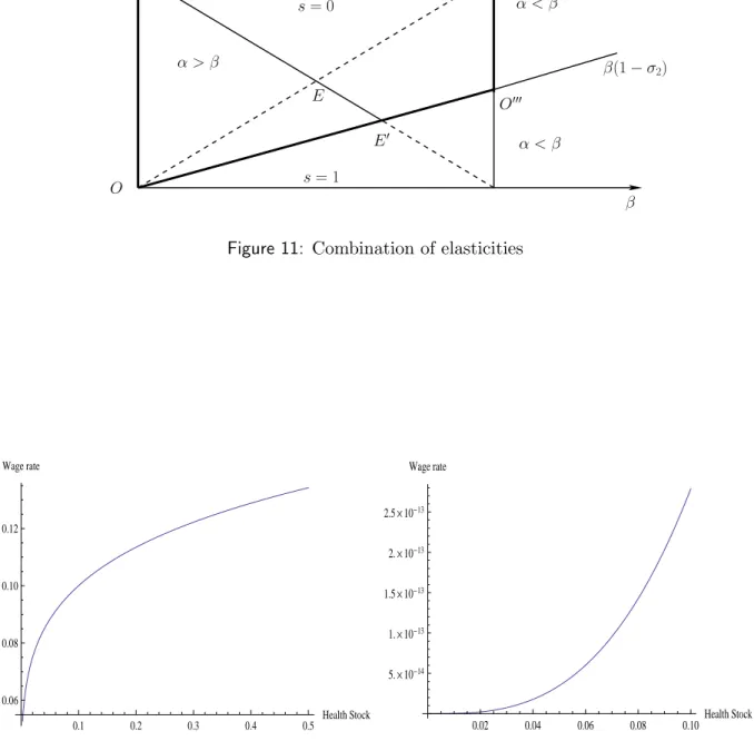
From the production side, we consider a representative firm with Cobb-Douglas technology for the function F with the refinement that productivity depends on health deep parameters. Moreover, we assume productivity in this sector as a function of the health stock.4 This leads to Y (z) = B (M (z)) F (K, L) where, Y (z), K (z) and L (z) are respectively the output, capital and labor, while B(M (z)) is the productivity as a function of the health stock M . Let the effective labor supply be N (z) = γ(M)L(z). The fraction γ(M) shall depend on the level of health, L(z) being the total labor input and γ(M ) is an increasing function. As productivity depends on the stock of health, B(M (z)) = a(z)γ(M )1−ϵwith 0 < ϵ < 1 and a(z) represents the technical progress which corresponds also to the global productivity. For the limit conditions of B(M ), the minimum level of health is assumed M = Mmin ≥ 0. Furthermore, B(Mmin) = a(z) if one assumes that γ(Mmin) = 1. We also assume that B(∞) = Mmax (which implies that the productivity cannot increase indefinitely) and BM M ≤ 0. Let us denote ˆk = KL the capital-labor
ratio. Then the output per labor is given by f (ˆk) = Y (z)L(z) = B(M (z))ˆk(z)ϵ. 2.2 Optimality
Individuals maximize lifetime utility as stated in Eq. (1), subject to the state variables ˙A(z) and ˙M (z) in Eqs. (2) and (3) respectively. The Hamiltonian of this optimal control problem is
4We thank two anonymous referees of the Journal for suggesting to make the productivity in the final sector as a function of the health stock and their suggestion to study the effect health not only on felicity but also on labor supply and wage income.
given by: H(C, m, M, A, λA, λM) = V { S [U (C(z)), φ(M (z))] , N [U (C(z)), φ(M (z))]}e−ρz + λA [ r(z)A(z) + w(z)φ(M (z))− C(z) − h(m(z))]e−ρz (4) + λM [ ψ(m(z))− δMM (z) ] e−ρz
The optimality conditions (where, to ease notations, the argument z is removed when it’s not necessary) associated to this problem are given as:
∂H ∂C(z) = e −ρz(−λ A+ UCVNNU+ UCSUVS) = 0 (5a) ∂H ∂m(z) = −e −ρzλ Ahm+ e−ρzλMψm = 0 (5b) ∂H ∂M (z) = e −ρz(− δ MλM + φM(wλM+ NφVN+ SφVS) ) = e−ρz ( ρλM − ˙λM ) (5c) ∂H ∂A(z) = e −ρz(rλ A) = e−ρz ( ρλA− ˙λA ) (5d) with the associated transversality conditions:
lim z→∞λA(z)e −ρzA(z) = 0 (6a) lim z→∞λM(z)e −ρzM (z) = 0 (6b)
The functions λA(z) and λM(z) are the costates and subscripts indicate the first derivative of
functions w.r.t mentioned arguments. The general dynamic system is given by: ˙ C(z) C(z) = − (r− ρ)(VNNU+ SUVS)− Ψ1M (z)φ˙ M Ψ2 UC C(z) (7a) ˙ m(z) m(z) = − Φ UC(VNNφ+ SUVS)(ψmh′m− hmψ′m) ψm m(z) (7b) ˙ M (z) M (z) = ψ(m(z)) M − δM (7c) ˙k k = B(M )ˆk ϵ−1−Cˆ k − ˆ m k − δ (7d)
where δ≥ 0 is the capital depreciation rate and w is the wage rate and:
Ψ1 = VSSU φ+ VNNU φ+ Nφ(VφφNU+ SUVSN) + Sφ(NφVSN+ SUVSS)
Ψ2 = U
′
C(VNNU + SUVS) + UC2(VφφNU2 + 2SUNUVSN + VSSU U + VNNU U+ SU2VSS)
Φ = UC(VNNφ+ SUVS) [wφMψm− (δM + r)hm] + φMψm(NφVN + SφVS)
Our objective consists in finding the optimal trajectories of the model key variables: consump-tion, investment in health, health stock and capital. Given the assumptions 1-4, our optimization program allows to get these optimal variables. It is worth noticing that it would have been inter-esting to incorporate infectious diseases and their modes of transmission in our dynamic setting to assess the impact of health on variables such as capital accumulation, consumption, wages, etc. Indeed, it is interesting to know how health deterioration may affect the existence of solu-tions to the maximization of welfare. As well documented in Goenka and Liu (2012) and Goenka et al. (2014), if this damage was done by infectious diseases, then a problem of non-convexity arises and one needs to check existence conditions for optimal solutions.5
5
We are very much grateful to a referee who pointed out to clarify the potential non-convexity issues in the study. Indeed, Goenka and Liu (2012) and Goenka et al. (2014) showed that given the internal propagation mech-anism of infectious diseases, there are non-convexities in the transmission process which make the optimization problem subtle.
In fact, Goenka and Liu (2012) and Goenka et al. (2014) discussed the optimal investment in health, in the light of the interaction between the transmission of diseases and the economy. If diseases affect the labor market, health investments choices also affect the transmission of diseases. Health expenditures lead to the accumulation of health capital and thus reduce the spread of diseases and improve convalescence and recovery from illness. However, the non-convexity of the dynamics of infection implies that one should be careful in implementing the optimal control techniques. Indeed, to characterize optimal solutions, the first order conditions (and the transversality conditions) of the Hamiltonian may be necessary but not sufficient. Then there may be jumps issues of state and co-state variables within the feasible set whereas the existence of optimal solutions relies on compactness of the set and absolute continuity of the state variables. In this study we do not make specific assumptions on the nature of diseases (infectious or not) as well as their transmission mechanism. Incorporating these mechanisms in our model will pose additional extra difficulties that we leave for future research while focussing on the equally difficult separability issue of preferences structure.
Some general remarks can be made before addressing the calculation of optimal trajectories. Firstly, Eq.(5a) gives the expected evolution of optimal consumption which can be disentangle into ˙C(z) = C1(z) + C2(z), with C1(z) = −(r−ρ)(VNNΨU2+SUVS)UC and C2(z) = Ψ1UC
˙
M (z)φM
Ψ2 . The term C1(z) denotes the Fisher conditions binding the slope of consumption trajectory to the difference between the time preference and interest rates. The term C2(z) reflects the interaction between the stock of health and consumption. When time increases, the stock of health shall move towards its minimum level, and the marginal loss of time health φM(M (z)) will reach its
maximum, thereby reducing consumption.
Secondly, the opportunity cost of health stock (or unit cost), can be retrieved from the Eq.(5b) as λM
λA = g(z). At equilibrium, the instantaneous user cost of health stock is equal to
the instantaneous marginal benefit from one-unit increase in the stock of health. The optimal health investment is determined by the intersection between the curves representing these two elements. We have not chosen an explicit specification for the cost function, but we can still derive some information from the expression of the opportunity cost of health, based on co-state variables. Thus, it can be shown from Eq.(5c) that :
g(M (z)) ( δM + r− ˙g(z) g(z) ) = φM [ w + 1 λA(0) (NφVN+ SφVS) e(ρ−r)z ] (8) The first part of this equality stands for the user cost of health capital, the form of which as can be seen is comparable to that of physical capital in the theory of investment. It is also termed ‘marginal efficiency of capita’ (Grossman, 1972). The second member is the effect on the utility of an increase in the stock of health. Thus, the user cost of health capital should be equal to the instantaneous marginal benefit of an increase in the stock of health. The relations (Eq.8) can be transformed into a differential equation g(t) which shows after solving that the opportunity cost is therefore proportional to:
g(M (z)) = ∫ ∞ z [ φM(M (x)) ( w + 1 λA(0) (NφVN + SφVS) e(ρ−r)x )] e−(δM+r)(x−z)dx (9)
This expression gives the present value of the benefits of health stock available on the remaining life. We will use the cost opportunity term later on in the penultimate section for policy purposes. In the next section, we address the case where the expression ofV is specified to have a separable term. We shall study the steady state and equilibrium dynamics of the model.
3
Additively separable preferences
The interaction between health and the ways it affects felicity has been so far investigated within additive structure preferences (Hall and Jones, 2007). As a result health status and consumption are additively separable functions implying that the marginal utility of consumption is indepen-dent from health status. While adopting this approach in this section, let’s remember that we add a final good sector to better understand the life cycle aspect agent’s behavior. In that case, the welfare function V turns to take the form:
V{S[U (C(z)), φ(M (z))], N [U (C(z)), φ(M (z))]}= S[U (C(z)), φ(M (z))] = U (C(z))+φ(M (z)) (10) We shall also resort to the constant relative risk aversion (CRRA) felicity function, which has the below functional forms for U (C(z)) and φ(M (z)), and a decreasing return in health investment for function ψ(m(z)): U (C(z)) = C(z) 1−σ1 1− σ1 and φ(M (z)) = M (z)1−σ2 1− σ2 (11) h(m(z)) = πm(z)α and ψ(m(z)) = bmβ (12)
with σ1 < 1, σ2 < 1, b > 0, β > 0, π > 0 and 0 < α < 1. Here σ1 is the inverse of elasticity of substitution between consumption at any two points in time, and σ2 denotes the same for health capital. U (C(z)) and φ(M (z)) are strictly increasing and concave respectively in C(z) and M (z). ψ(m(z)) represents the health investments function, which is concave in m(z), reflecting the assumed diminishing returns in health investment. π is the productivity or efficiency of health investment. Increased health care productivity not only shifts the health production function upward, but causes each unit of health care to have a larger contribution to health as well. Ehrlich and Chuma (1990) also assumed that consumers choose death when the stock of capital M (z) is under a certain minimal level Mmin. All these functions fulfilled the assumptions 1-3.
3.1 Steady state
The first order conditions with respect to C(z) and A(z) from the Hamiltonian (4) yield the traditional Euler equations. One can see that equations (7a) and (7b) turn to be respectively:
˙ C(z) C(z) = 0⇐⇒ (r − ρ)SUVS− [VSSU φ+ SφSUVSS] ˙M (z)φM = 0 (13) and ˙ m(z) m(z) = 0⇐⇒ UCSU[wφMψm− (δM + r)hm] + φMψmSφ= 0 (14) Thus, Eq.(13) defines a differential equation in M (t) which allows to find the value M∗(t) at equilibrium. The latter can then be introduced into (14) to find consumption equilibrium C∗(t) given that the stock of health and investment are linked by the relation (7c). More specifically, using Eqs.(11) and (12) we obtain the demand side system:
˙ C C = r− ρ σ1 (15a) ˙ m m = ( − φMψm2 + UC ( (r− ρ)hmψm+ ((δM + ρ)hm− wφMψm ) ψm ) UCm(ψmh′m− hm)ψm′ (15b) ˙ M M = bmβ M − δM (15c)
Proceeding with the final sector, remember that f (ˆk) = Y (z)L(z) = B(M (z))ˆk(z)ϵ. Then, the maximization of the profit function under perfect competition allows to equalize the marginal cost of each factor with its marginal benefit. Therefore,
r(z) = ϵB(M (z))ˆk(z)ϵ−1− δ (16)
w(z) = f (ˆk(z))− ˆk(z)f′(ˆk(z)) = (1− ϵ)B(M(z))ˆk(z)ϵ (17) Combining the demand and the supply sides, we can now characterize the equilibrium of the economy. We can write
˙ˆk(z) = B(M(z))ˆk(z)ϵ− ˆC(z)− ˆm(z)− (δ + n) ˆk(z) (18)
where ˆC(z) and ˆm(z) are respectively the consumption and health expenditure per labor, and n is the population growth rate. Therefore, the dynamics of the economy can be summarized by the following non-trivial four dimensional system:
˙ˆ C(z) ˆ C(z) = r(z)− ρ σ1 (19a) ˙ˆ m(z) ˆ m(z) = δM + r α− β − bβ(w + Cσ1)M−σ2mβ−α πα(α− β) (19b) ˙ˆ M (z) = bmβ− δMM (z)ˆ (19c) ˙ˆk(z) = B(M(z))ˆk(z)ϵ− ˆC(z)− ˆm(z)− δˆk(z) (19d)
including ˆk(0) and ˆM (0) as given and in addition the transversality conditions. The steady-state values of ˆC, ˆm, ˆM , and ˆk are obtained by equalizing C, ˙ˆ˙ˆ m,M ,˙ˆ ˙ˆk to zero. We obtain:
b C = w 1− ϵ ( 1− ϵ r + δ ) − ( δM b )1 β c Mβ1 (20a) b m = ( δM b )1 β c Mβ1 (20b) c Mσ2−1+αβ = b ( b δM )−σ2 β π(δM + r)α [ w + ( w 1− ϵ ( 1− ϵ r + δ ) − ( δM b )1 β c Mβ1 )σ1] (20c) ˆ k = B(M )1−ϵ1 ( δ + ρ ϵ ) 1 ϵ−1 (20d) The following proposition characterizes the solution of the system.
Proof. See Appendix A.
The next proposition states the comparative statics of the model as regard the effect of health stock on the wage rate. It also states the conditions of existence for the equilibrium and the stability of the dynamic system.
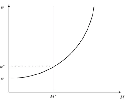
Proposition 2 The effect of health stock on the wage rate is positive provided that α≥ β(1−σ2) and α > β. Moreover, there exists a minimum wage rate w0 from which the stock of health impacts positively on the wage rate.
Proof. See Appendix A.
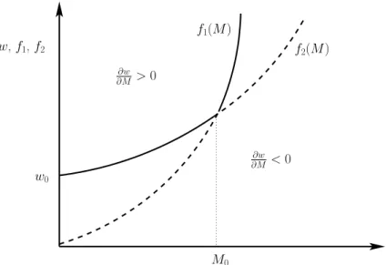
The condition in the proposition means that the ratio of the elasticities of the cost of health and health investment is greater than the elasticity of the production function of health. In addition, for the stock of health to have a positive effect on the wage rate, it is necessary that the wage rate remains higher than a minimum level w0. We seek for conditions under which the minimum level w0 can be determined. Relying on Eq.(A-1; see Appendix A), settingWN ≥ 0 and WD > 0 is equivalent to writing respectively w≥ f1(M ) and w > f2(M ) where
f1(M ) = (r + δ)(1− ϵ) r + δ− ϵ ( δM b )1 β Mβ1 + ( b δM )σ2( δM b )−1 βM−1+α−β+βσ2β π(δ M+ r)α(β− α − βσ2) bβσ1 1 −1+σ1 f2(M ) = (r + δ)(1− ϵ) r + δ− ϵ [( σ1 ϵ− r − δ (ϵ− 1)(r + δ) ) 1 1−σ1 + ( δM b )1 β Mβ1 ] Insert Figure 1
Figure 1 shows the curves f1(M ) and f2(M ). The dash line curve from the origin becomes solid line from M0, while the solid curve from w0 becomes dash line from M0. We have:
M0 = r+δ−ϵ (1−ϵ)(r+δ) ( b δM )1 β+σ2 π(δM + r)α(α− β + βσ2) bβ β 1−α+β−βσ2 (21) w0 = (r + δ)(1− ϵ) r + δ− ϵ [ σ1 r + δ− ϵ (1− ϵ)(r + δ) ] 1 1−σ1 (22) In fact, the influence of the stock of health on the wage rate is positive in the area bounded by the y-axis and the solid curve, knowing that the minimum ordinate is w0. This domain is sup(f1, f2)(M ). It is therefore possible that the stock of health has a negative effect on the wage rate and it is more related to the specification of the welfare function. Indeed, in the case of additive preferences we find that SU φ and VSS from Eq.(13) vanish. As a result, the solution
M∗(z) is derived from Eq.(14). Relying on Eq.(7b), the expression of the wage rate is obtained as: w(M∗(z)) = (δM + r)hm[m ∗(z)] φM[M∗(z)]ψm[m∗(z)]− Sφ[M∗(z)] UC[C∗(z)]SU[C∗(z)] (23) where the variables m∗(z) and C∗(z) are expressed in function of M∗(z).
This result calls for some comments. There is a consensus on the positive effects of health on growth and development. Particularly in developing areas such as in Africa where improving the quality of health is crucial. Gallup and Sachs (2001) estimated that elimination of malaria in sub-Saharan Africa would allow the continent to achieve an annual average growth of 2.6%. However, it is not empirically proven convincingly that health has a positive impact on growth and development. Indeed, most studies that have examined this impact do not have a general equilibrium perspective, which prevents them grasping the global dimension of the issue, in-cluding possible adverse effects of health (Acemoglu and Johnson, 2007). Our work helps to fill two important theoretical gaps in the literature. The first vacuum is the absence of a compre-hensive approach, which shows the role of health in a flexible theoretical framework, without introducing morbidity constraints or constraints related to demographic pressures of the popu-lation. Hence our general equilibrium approach can show that the economic effects of health, measured through the wage rate (and therefore productivity) may be positive, but only under certain conditions, especially related to quality of health and costs of health investments.
The second theoretical gap is evidence of negative effects of health on the economic sphere. Acemoglu and Johnson (2007) showed empirically that the effects of health (measured by longevity) on growth of GDP per capita can be negative. Relying on a neoclassical growth model, our study provides a theoretical basis to this finding. Intuitively, a high stock of health may well have a negative effect on the wage rate if economic growth (and hence the distribution of income) is reduced due to the aging population for example, or because of high opportunity cost in health spending, which harm economic sectors. This is also possible, if improved health leads to a reduction of capital per capita, and thus lower levels of income per capita.
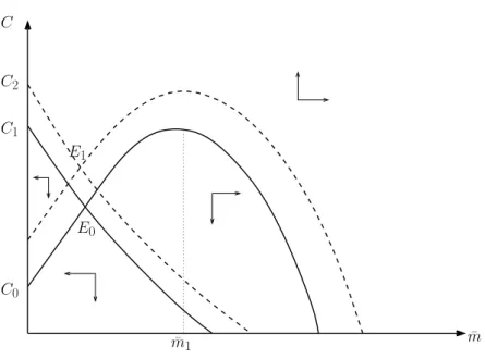
3.2 Phase diagrams
Let us now study the equilibrium dynamics of the system with phase diagrams. To this end, we express the variable in units of physical capital by setting: c = Ck, m = mk and M = Mk. It follows that the variables follows the system:
˙c c = r− ρ σ1 − r + δ(1− ϵ) ϵ + c + m (24a) ˙ m m = δM + r α− β − bβ(w + kσ1cσ1) ¯M−σ2mβ−αkβ−α−σ2 πα(α− β) − r + δ(1− ϵ) ϵ + c + m (24b) ˙ M M = bmβkβ−1 M − δM− r + δ(1− ϵ) ϵ + c + m (24c)
The condition in the proposition ensures also the existence and uniqueness of the steady state and guarantees the stability. Relying on the implicit behavior of ¯m and parameters conditions, we prove below that this leads to the the existence and uniqueness of the solution. We are now interested in the changes in the equilibrium, when some health parameters are modified. We propose a geometrical representation by drawing the phase diagrams associated to the system (24a)-(24c). The diagrams are plotted on different planes while fixing each of the variables. Lemma 1 elaborates on the phase diagrams in Figures 2, 3 and 4.
Lemma 1 We have:
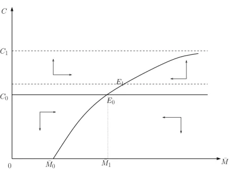
i) For ¯m fixed, the curve ˙c = 0 is a horizontal line and the locus ˙¯M = 0 is an increasing and concave function. Moreover we have limM¯→∞c = b2 for b2 given.
ii) For c fixed, the curve ˙¯M = 0 monotonically increases and the locus ˙¯m = 0 is a decreasing and convex function with limm¯→0M = 0 and lim¯ m¯→b−M =¯ ∞.
iii) For ¯M fixed, the curve ˙c = 0 is a decreasing straight line and the locus ˙¯m = 0 is an increasing function over a real support and it decreases monotonically from ¯m0.
Insert Figures 2, 3, 4
Fixing ¯m = ¯m0 leads to the phase diagram onto the plane (c, ¯M ) (see Figure 2). We have two curves. The first one ( ˙c = 0) is independent of the stock of health. An increase of the rate of health depreciation (δM) implies a shift of the second curve ( ˙¯M ) towards the left. This curve
is increasing with both consumption and health. The shift induces a decrease of health from the steady state E0 to a new one E1, where consumption remains constant.
The second phase diagram in Figure 3 is plotted onto the plane ( ¯m, ¯M ) by fixing c. The two curves are increasing with the variables ¯m and ¯M ), but the stock of health grows faster than the flow of investment. An increasing rate of health depreciation leads to a high reduction of the stock of health which is not fully compensated by the investment. So the two curves shift down to the steady state E1.
Fixing ¯M gives the third diagram in Figure 4 on the plane (c, ¯m). Relying on the equation ( ˙c = 0) there is a linear relation between the flow of investment and consumption. The stable manifold is in the zones on the left hand side of E0 above the curve and the right hand side of E0 below the curve. Within these two zones, the trajectories converge to the steady state values. An increase of δM generates a higher level of investment flows. Moreover, a crowding
effect appears and consumption jumps backward from the first steady state E0 to the second one E1.
4
Multiplicative preferences
In the previous section, consumption and health enter into the utility function in an additive way. As a result, the marginal utility of consumption can be independent from health, which reflects a strong limitation as consumption is also crucial for health. The alternative model in this section seeks to account for this important aspect. The welfare function V takes now the form:
V{S[U (C(z)), φ(M (z))], N [U (C(z)), φ(M (z))]}= N [U (C(z)), φ(M (z))] = U (C(z))φ(M (z)) (25) In order to be able to compare consistently the results, we use the same CRRA felicity functional forms for U (C(z)) and φ(M (z)) as in Eq.(11), as well as the same health functions h(m(z)) and ψ(m(z)) in Eq.(12). Also the final sector description is the same. Given this new set-up, we can study the steady state and equilibrium dynamics of the non-separable multiplicative preferences model.
4.1 Steady state
Here, Eqs.(7a)-(7b) turn to be respectively ˙ C(z) C(z) = 0⇐⇒ (r − ρ)VNNU− [VNNU φ+ NφNUVφφ] ˙M (z)φM = 0 (26) and ˙ m(z) m(z) = 0⇐⇒ UC[wφMψm− (δM + r)hm] + φMψm = 0 (27)
As previously, Eq.(26) defines a differential equation in M (t) which allows to find the value M∗(t) at equilibrium. The latter can then be plugged into (27) to retrieve consumption equilibrium C∗(t) thank to relation (7c). The dynamics of the economy is driven at equilibrium by the following system: ˙ˆ C(z) ˆ C(z) = (r− ρ)M(z) +(δMM (z)− bm(z)β ) (σ2− 1) M (z)σ1 ˙ˆ m(z) ˆ m(z) = 1 πα(α− β)(1 + σ1)M (z)1+σ2) [ π(δM + r)αM (z)1+σ2(1 + σ1) − bβm(z)β−α(wM (z)(1 + σ 1) + C(z)M (z)σ2)(1 + σ2) ] ˙ˆ M (z) =−δM + bmβ m(z) ˙ˆkz= B(M (z))ˆk(z) ϵ − ˆC(z)− ˆm(z)− δˆk(z) (28)
with ˆk(0) and ˆM (0) given, plus the transversality conditions. The steady-state values of ˆC, ˆm, ˆ
M , and ˆk are obtained by equalizingC, ˙ˆ˙ˆ m, M ,˙ˆ ˙ˆk to zero. We have:
b C = w 1− ϵ ( 1− ϵ r + δ ) − ( δM b )1 β c M1β (29a) b m = ( δM b )1 β c Mβ1 (29b) c Mσ2+αβ−1 = bβ π(δM+ r)α ( δM b )β−α β [ w + ( w(2(r + δ)− δϵ) (r + δ)(1− ϵ) − ( δMM b )1 β) c Mσ2−1σ2− 1 σ1− 1 ] (29c) ˆ k = B(M )1−ϵ1 ( δ + ρ ϵ ) 1 ϵ−1 (29d)
The following results hold: Proposition 3
i) The dynamic system (29a)-(29d) admits a stable solution.
ii) The effect of health stock on wage rate is positive provided that β(1− σ2)≤ α < β. Proof. See Appendix A.
To study how the wage rate behaves in this case, on can rely on Eq.(29c). Solving the latter with respect to wage leads to:
w(M ) = ( δM b )α β M−1+σ2π(δ M + r)α Mα β +δM (δM b )− αβ(δM M b )1 ββ(−1+σ 2) π(δM+r)α(−1+σ1) δMβ ( 1 +M−1+σ2(2r+2δ−δϵ)(−1+σ2) (r+δ)(1−ϵ)(−1+σ1) ) (30)
which is fully expressed in terms of M . On can check (see Appendix A, Proof of Proposition 3) that w(M ) here is an increasing function of M .
As we can see from Propositions 2 and 3, the conditions for the wage rate be related to health stock are different. Both cases share a common condition which is α ≥ β(1 − σ2). However,
whereas in the additive case one needs in addition α > β, the multiplicative preference requires α < β leading to the inequality condition in Proposition 3. The latter states that the ratio of the elasticities of the cost of health and health investment must be lower than the elasticity of the production function of health. The stock of health has throughout a positive effect on the wage rate. Compared to the additive preference, we no longer have the domain of negative effect of stock of health on the wage rate which was displayed in Figure 1. Formally, this result clearly follows from the structure of preferences. However, from an economic and empirical perspective, how could one explain this change in wage rate with respect to preferences.
In the case of additive preferences, health status and consumption are additively separable in the utility function implying that the marginal utility of consumption is independent from health status. This does not fit in for instance with the notion that good nutrition is also important for health. Indeed, healthy eating might lead to a reduction in mortality from chronic illness, and appropriate dietary advice can prevent physical and mental deterioration and improve the quality of life. Evidence from Friis and Michaelsen (1998) supports this rationale. Therefore, consumption is also crucial for health. The multiplicative non-separable preferences highlights the interaction between consumption and health although it is very difficult to slice on the net effect of a high health deterioration rate and low health productivity on health investment.
Another way to interpret the common relationship α≥ β(1 − σ2) between the Propositions 2 and 3 is to consider the changes in inter-temporal substitution of health with respect to health investment and the cost of that investment. Indeed it appears that the higher the health investment (i.e. β), the lower the elasticity of substitution. Inter-temporal substitutability of health can become zero if the cost of investment in health become increasingly high. In order to improve substitutability of health stock over time, justifying a reduction in inertia of household health behavior, there must be a combination of two phenomena: a gradual decrease in elasticity of health production and a simultaneous increase of the costs of health investment. This may seem against intuition. However, it should be noted that if households determine the level of current health stock taking into account its level in the previous period, this may affect the future marginal utility of health stock. Indeed, any increase in the level of health of the current period increases the future marginal utility of health. The effect of inter-temporal substitution between present and future stocks becomes weak if health habits are persistent. In this case, the representative household has to spend much more wealth between the current period and the future period to improve the stock of future health. And even with a low rate of health depreciation, the costs of health investments become increasingly high.
4.2 Phase diagrams
We now elaborate on how the health parameters affect the steady-state values, notably the health investment variable and the consequences on consumption, capital stock and savings. To this end, we study the equilibrium dynamics of this economy. Using the same variable definition above, the dynamical system is computed as:
˙c c = −(r − ρ)M + (−1 + σ2)(−δMM + bmβk−β+1) −σ1M − r + δ(1− ϵ) ϵ + c + m ˙ m m = c σ1m1−αMσ2k−σ2+α−1 (( bm−1+βM−σ2kσ2−β+1 ( c1−σ1 −1 + σ1 + wc−σ1 ( M1−σ2kσ2−1 −1 + σ2 )) + π(−δM − r)αc−σ1m−1+αk1−α ( M1−σ2kσ2−1 −1 + σ2 )) (−1 + σ2) )/ (πα(α− β)((−Mk−1)) ) −r + δ(1− ϵ) ϵ + c + m ˙ M M = bmβkβ+1 M − δM − r + δ(1− ϵ) ϵ + c + m (31)
Here again, we turn to analysis of the changes in the equilibrium when some health parameters are modified. Lemma 2 documents on the phase diagrams in Figures 5, 6 and 7 which are associated to the system Eq.(31).
Lemma 2 We have:
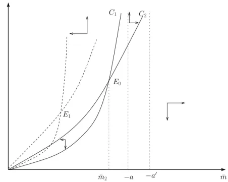
i) For ¯m fixed, the curve ˙c = 0 is a horizontal line and the locus ˙¯M = 0 is an increasing and concave function, with limM¯→∞c = a′ for a′ given.
ii) For c fixed, the curves ˙¯m = 0 and ˙¯M = 0 are convex and monotonically increasing with limm¯→aM =¯ ∞ and limm¯→a′M =¯ ∞ for a and a′ given.
iii) For ¯M fixed, the curve ˙c = 0 is decreasing and the locus ˙¯m = 0 is an increasing function and it decreases monotonically from ¯m1.
Insert Figures 5, 6, 7
We fix ¯m and get the first diagram in Figure 5 onto the plane (c, ¯M ). As for the additive case, the curve ˙c = 0 doesn’t dependent on the stock of health ¯M . The consumption depends though only on the flow of investment and on the rate of health depreciation. The curve ˙¯M = 0 is concave and increases with both variables. Starting from the steady state E0, an increase of δM shifts upward the level of consumption, leading to the final equilibrium point E1. The depreciation of health reduces the stock of health, but this reduction is compensated by the shift of consumption. The result is a net increase of health.
The second phase diagram in Figure 6 is plotted onto the plane ( ¯m, ¯M ) by fixing c. The two curves are increasing with the variables ¯m and ¯M , but the stock of health grows faster than the flow of investment. An increasing rate of health depreciation leads to a high reduction of the stock of health which is not fully compensated by the investment. So the two curves shift down to the steady state E1.
The third diagram in Figure 7 is obtained onto the plane (c, ¯m) by fixing ¯M . There is a linear relation between c and ¯m that gives the monotonically decreasing curve. An increase of the depreciation rate shifts upward the consumption and the flow of investment in health on the curve ˙c = 0. We have the same with the curve ˙¯m = 0. The final steady state is reached at E1 where both variables increase.
Let us discuss insights from the equilibrium dynamic considering the effects of parameters in the different models and taking into account the dynamics of transition. We assume the economy is on balanced growth path when a parameter varies, and we analyze the adjustments to the new
equilibrium path. Let’s take the example of the phase diagram where we consider a variation of the rate of depreciation of health δM. Fixing ¯m, the phase diagrams are obtained on the plane
( ˙c, ˙M ) of Figures 2 and 5 wherein there are two curves for the additive and multiplicative cases. The first ones ( ˙c = 0) are independent of the stock of health. The curves M = 0 are concave and grow with both variables. In the case of the separable utility, an increase in the rate of impairment of health implies a movement of the second curve ( ˙M = 0) to the left. This induces a reduction of the health by the move from the stable equilibrium E0 to a new equilibrium E1 where consumption remains constant. Conversely, in the multiplicative case, starting from the steady state E0, an increase in δM shifts up the level of consumption, leading to the end point
of equilibrium E1. Impairment of health reduces the stock of health, but this decrease is offset by the increase in consumption. The result is a net increase in the stock of health.
Fixing ¯c gives both Figures 3 and 6 on the plane ( ˙m, ˙M ) that relate the stock of health to health investment. For the additive as well as for the multiplicative case, the curve ( ˙M = 0) increases, but the health stock increases faster than investment flows. When impairment of health increases, this implies a lower level of health stock. The curve m = 0 moves to the left. But the flow of investment increases, which means that the final steady state is reached when the curve ˙M = 0 shifts to the right. The final state of equilibrium point is E1 where the stock of health is lower than the first equilibrium point E0.
Fixing ¯M produces Figures 4 and 7 in the plane ( ˙c, ˙m). For the additive case, starting from the equation ( ˙c = 0) we see that there always exists a linear relationship between the flow of health investments and consumption. The trajectories converge to equilibrium from the areas of stability on the left values of E0. An increase in δM generates a high level of investment
flows. In addition, a crowding effect appears and consumption reduced from E0 to E1. For the multiplicative case, the equilibrium is reached at point E1 where both variables increase simultaneously.
5
Convex combination of preferences
In this section, we combine both cases in a general framework. Indeed, it is likely that be-tween purely additive and multiplicative preferences, there might a range of choice in bebe-tween depending parameter link that may drive agents’ behavior. The welfare function V takes now the form:
V (·) = sU(C(z))φ(M(z)) + (1 − s)[U(C(z)) + φ(M(z))] (32) and s is a parameter link such that 0≤ s ≤ 1. If s = 1 then the individual preference becomes additive and for s = 0 it is multiplicative.
The dynamic system then is obtained by the Eqs.(7a)-(7d). The optimization equations (5a)-(5d) provide sufficient conditions for maximizing welfare because of the concavity of the utility function, the production of health and health investment. The Hamiltonian is a concave function of the state variables and control variables. The following result holds:
Proposition 4 The equilibrium values of health stock are located on a trajectory which is time dependent and given by the relation:
c M (z, s) = [ θ0(s) + θ1e−z(r−ρ) ] 1 1−σ2 (33) with θ0(s) =−s11−σ−s2 and θ1 = ¯λ(1− σ2) where ¯λ is an integration constant.
Proof. See Appendix A.
Proposition 4 is interesting as it shows that the balance health variables cM and ˆm can be ex-pressed as a function of time, regardless of other real variables such as consumption and capital per capita. However, as Eqs.(7a)-(7d) of the general system establish the links between the variables in the model, the equilibrium expression of these variables can be recovered. But this approach is analytically complicated if not impossible. Moreover, as we have documented in the Appendix B, studying analytically the equilibrium dynamics of the model in the case of convex combination of preferences is unbearable.
The expression of health investment at equilibrium m(z) is then obtained as:b b m(z) = ( δM b )1 β[ θ0(s) + θ1e−z(r−ρ) ] 1 β(1−σ2) (34) Relying on Eq.(7b) and using Sφ[M∗(z)] = (1− s)φM[M∗(z)] and SU[C∗(z)] = (1− s)UC[C∗(z)]
the expression of wage rate is obtained as: w(M∗(z)) = (δM + r)hm[m ∗(z)] φM[M∗(z)]ψm[m∗(z)]− φM[M∗(z)] U2 C[C∗(z)] (35) where M∗(z) and m∗(z) are replaced by their expressions.
Figure 8 shows the evolution of the stock of health and health investment. The curves depart from an initial value at time z = 0 given by the expressions cM (0, s) and m(0, s) as describedb below. As in the model of Ehrlich and Chuma (1990), cM and m are decreasing and tend to ab minimum.
Insert Figure 8
Furthermore, Proposition 4 allows us to study the limits behavior of stock and investment in health. We can distinguish two cases: i) infinite horizon (z → ∞) and ii) finite horizon (z → T ). In the first case, taking the limit of Eqs.(33) and (34), we obtain respectively: limz→∞M (z, s) =c
c M (∞, s) = [θ0(s)] 1 1−σ2 and lim z→∞m(z, s) =b m(b ∞, s) = (δMb ) 1 β[θ 0(s)] 1 β(1−σ2). For z = 0, we have cM (0, s) = [θ0(s) + ¯λ(1− σ2)] 1 1−σ2 and m(0, s) = (b δM b ) 1 β[θ 0(s) + ¯λ(1− σ2)] 1 β(1−σ2). Infinite
horizon also implies high health deterioration meaning that health will tend to its minimum. It follows that cMmin(∞, s) = [θ0(s)]
1 1−σ2 and mb min(∞, s) = (δMb ) 1 β[θ 0(s)] 1 β(1−σ2).
The case of finite horizon is of particular interest because it provides the expression of the time limit for the stock of health to be low, and that life ends at some T (·, s). We have:
lim z→T c M (z, s) = cM (T, s) = [ θ0(s) + ¯λ(1− σ2)e−T (r−ρ) ] 1 1−σ2 (36) When T is reached, health reaches its minimum given by Eq.(36). Figure 9 displays the graph for that case. cM (T, s) decreases and reaches its minimum at horizon T (s).
Insert Figure 9
An interesting theoretical issue is what would be the value of time horizon T , if the min-imum level of health is known. Let’s recall our approach to better understand the theoretical
importance of the finite time horizon. In the model, we looked for the optimal paths of consump-tion, capital and health variables for infinite horizon. The framework of convex combination of preferences leads to purely temporal expression of health stock and health investment. These variables depend on what we call the structure parameter or convexity of the model, s. The latter allows to balance the model between the two polar cases: additive and multiplicative welfare function. The benefit of having optimal variables that are expressed in terms of time is that one can identify the limits which in turn depend on the model parameters. Therefore, setting s, and making assumptions about the minimum value of the stock of health, we can infer a temporal horizon that represents longevity, i.e. life duration over which health keeps economic activities of work, consumption and investment. Suppose the minimum stock is not zero, then T can be obtained from Eq.(36) for cM (T, s) = cMmin(s), and be expressed in terms of other model parameters as: T = 1 r− ρln ( ¯ λ(1− σ2) c Mmin(s)− θ0(s) ) = T0+ 1 r− ρln ( 1− σ2 c Mmin(s) + s1−σ2 1−s ) (37)
with T0 = r−ρ1 ln ¯λ. The study of function T with respect to parameters is interesting from two points of view. First, this horizon should ideally be farthest from zero as possible. Therefore, it is crucial to understand the role of each parameter to achieve this goal. Secondly, we have not explicitly sought optimal longevity as in Ehrlich and Chuma (1990). However, our approach leads to a model of optimal lifetime which generalizes Ehrlich and Chuma (1990). Indeed, as the authors, we find the same parameters that determine lifespan. In addition, here, lifespan also depends on the way welfare is chosen, i.e. parameter s. If we elaborate only on the effect of σ2 parameter, we have the following representation of T :
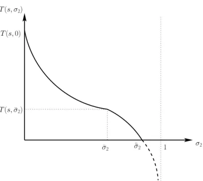
Insert Figure 10
In Figure 10, ¯σ2 = 1− (12s−s)Mminc (s) and ¯σ2¯ = 1− ¯λ(1(1−s)−s−s) Mminc (s) and T (¯σ2, s) is given by Eq.(37) evaluated at ¯σ2. Figure 10 also shows interesting aspects of the modeling. First of all, observe the vertical dotted line that stresses the constraint σ2 < 1. The longevity T curve shows a convex-concave shape. Indeed, the first portion of the curve which departs from T (s, 0) decreases convexly to reach the inflection point (T (¯σ2, s), ¯σ2) where the curve becomes concave till the point ¯σ¯2. Therefore, longevity is a decreasing function of the elasticity of inter-temporal substitution of health σ2. We also see that as long as σ2< ¯σ2¯ , lifespan is strictly positive. This indicates that there is a maximal bound for σ2 beyond which the stock of health is minimal. Thus, the choice of σ2 will impact the longevity modeling. Indeed, if σ2 ∈]¯¯σ2, 1[, longevity is zero, this means that the stock of health has no effect on real variables. As a result, there is no longer life: cM (z, s) = cMmin(s) = 0 for all z. However, if one chooses σ2 ∈]¯¯σ2, 1[, it is still possible to give a positive value to T provided to identify the structural parameter s which gives more weight to either the additive preference (s → 0) or the multiplicative one (s → 1). For s = 1 (multiplicative), we have ¯σ2 = ¯σ¯2 = 1. So one can choose σ2 in the range [0, 1[ and therefore T > 0. In other words, opting for multiplicative preferences rules out the problem of existence of T . However, if an additive preference (s = 0) is chosen, one should care about the issue of existence of T .
Some comments related to Propositions 2, 3 and 4 are in order. In economic theory, the effect of health quality care is often approached indirectly. Indeed, it is straightforward to measure health inputs and the indirect effects of health on the economy (through indicators
that are positively correlated with good health conditions, such as increased life expectancy, low morbidity rates, etc.). Although the quality of health is not directly measurable, our model allows to specify conditions for good health, by connecting three quantitative factors, namely health production, health investment and health costs. We have shown that the elasticities (α, β and σ2) of these three variables work together to define how health status influences labor. The model enables us to link the evolution of wage rates with respect to health. The transmission belt between the wage rate and health is labor productivity. As better health conditions enhances human capacities, the values created in the production process are improve in turn.
Two problems arise: those of causality and indeterminacy. There is a causality problem because when wage rates become too high, the most productive agents, that is to say, those with higher wages, consume more and more goods that improve health. Thus, causality can pass from greater labor productivity to better health, not from health to productivity. This is typically a reverse causality issue. The indeterminacy arises with the model specification. Indeed, there are values of the elasticities (α = β) for which the model may not have equilibrium and the influence of health on the wage rate becomes indeterminate. This also coincides with the fact that the opportunity cost of health stock becomes time independent. Figure 11 shows the combinations of parameters α and β that allows our models to have solutions.
Insert Figure 11
The axis OO′ makes an angle of 45◦ with the axis Oβ and the combination solutions which have the properties of additive and multiplicative case is delimited by the bold lines of the trapezium (OO′O′′O′′′), once the parameters α and β are set. On one hand, this is actually a combination of points belonging to the surfaces of triangles OO′O′′ (additive preferences) and OO′′O′′′ on the other hand (multiplicative preferences). These points are on the segment O′E′. However, the intersection points E with the segment OO′′ are excluded from the model because they check the equality condition α = β.
It is worth to notice a recurring problem in the field of health investment. Indeed, usually the aim is to look for the second best optimum in order to conciliate efficiency and social equity by proposing an optimal tax system and subsidies. Indeed, according to neoclassical theory, efficiency is reached when all agents behave competitively, and optimal allocations are then first best. Equity can be achieved through redistribution of income between healthy workers, workers whose health stock is low, and investors. This would have allowed us to disconnect the ‘final distribution of health stock’ of that resulting from the ex-post prices and elasticities structure of production and investment. But at this stage of our model, the issue is not that of equity. Our intuition is that we could have come up with explanations for the difference in results between the additive and the multiplicative preferences. We leave this for future research.
6
Opportunity costs of health
In this section, we compare the opportunity costs of health investment under the three alternative preferences. Such comparison is useful for policy analysis. Indeed, for a decision maker, it is interesting to know what investment alternative is the most effective in face of limited resources. Actually, for public policy reasons, the health sector is in competition with others economic sectors. A a result, the less costly alternative might be privileged. However, cost is only one input of the decision, as the latter should also consider the expected benefit from the investment in order to have a full picture of the decision options. This usually leads to an empirical cost
benefit analysis. Our objective here is to shed a theoretical light on the cost aspect of that mechanism.
In section 2, we established in Eq.(9) the expression of the opportunity cost in a very general way. The latter provides the present value of the benefits of health stock available on the remaining life. We can derive the analogue of Eq.(9) for each type of preference. In the additive case, we have: g1(M (z)) = ∫ ∞ z [ φM(M (x)) ( w(M ) + 1 λA(0) (SφVS) e(ρ−r)x )] e−(δM+r)(x−z)dx (38)
where the wage rate w is given by Eq.(20c). For multiplicative preference, we have: g2(M (z)) = ∫ ∞ z [ φM(M (x)) ( w(M ) + 1 λA(0) (NφVN) e(ρ−r)x )] e−(δM+r)(x−z)dx (39)
where the wage rate w is given by Eq.(30). For the convex combination of preferences, we have: g3(M (z)) = ∫ ∞ z [ φM(M (x)) ( w(M ) + 1 λA(0) (sU + (1− s)) e(ρ−r)x )] e−(δM+r)(x−z)dx (40)
where the wage rate w is given by Eq.(35). The functions or distributions g1(M (z)), g2(M (z)) and g3(M (z)) for 0≤ z ≤ ∞ can be compared using the notion of stochastic dominance. Define the distributions gi(M (x)) for preferences structure i = 1, 2, 3 (additive, multiplicative and
convex combination respectively) as gi(M (x)) = φM(M (x)) ( wi(M (x)) + 1 λA(0) Φie(ρ−r)x ) e−(δM+r)(x−z) (41)
where Φ1 = SφVS, Φ2 = NφVN and Φ3= sNφVN + (1− s)SφVS. We can then write
gi(M ((z)) =
∫ ∞
z
gi(M (x))dx
implying that gi(M (z)) is the complementary cumulative distribution of M (x). That is gi(M (z)) =
1− F (M(z)) where F (M(z)) =∫−∞z gi(M (x))dx is the cumulative distribution of M (x).
Definition 1 A complementary cumulative distribution (CCD)F is said to first-order stochas-tically dominate (FOSD) another distribution G if and only if F (x) ≥ G (x) for all values of x. A CCD F is said to second-order stochastically dominate (SOSD) another distribution G if and only if ∫z∞F (x)dx ≥∫z∞G (x)dx for all z, with a strict inequality for at least some values of z. Note that ifF and G in the Definition 1 were cumulative distributions rather than CCDs then the inequalities would be reversed. In relation to the expressions of opportunity costs, gi(M (z)) FOSD gj(M (z)) for i̸= j implies that the opportunity cost under preference structure
i is greater than the opportunity cost under preference structure j for all values of M (z). The following result holds:
Proposition 5 Let the structure of opportunity costs be as in Eqs.(38-40) and let ⟨M(x)⟩wi
denote the expected value of M (x) under wage rate distribution wi(M (x)). If C(x)≥ (1−σ1)
1 1−σ1
for all x, then:
(i) g2(M (z)) FOSD g1(M (z)) whenever w1(M (x)) = w2(M (x)) for all M (x) or ⟨M(x)⟩w2 ≥