HAL Id: hal-02929399
https://hal.univ-grenoble-alpes.fr/hal-02929399
Preprint submitted on 3 Sep 2020HAL is a multi-disciplinary open access
archive for the deposit and dissemination of sci-entific research documents, whether they are pub-lished or not. The documents may come from teaching and research institutions in France or abroad, or from public or private research centers.
L’archive ouverte pluridisciplinaire HAL, est destinée au dépôt et à la diffusion de documents scientifiques de niveau recherche, publiés ou non, émanant des établissements d’enseignement et de recherche français ou étrangers, des laboratoires publics ou privés.
To cite this version:
Hisashi Nakahara, Qing-Yu Wang, Manuel Hobiger, Takashi Hirose. Statistical characteristics of seismic velocity changes measured by seismic interferometry. 2020. �hal-02929399�
Statistical characteristics of seismic velocity changes measured by seismic interferometry
Journal: Geophysical Journal International Manuscript ID GJI-20-0379
Manuscript Type: Research Paper Date Submitted by the
Author: 16-Apr-2020
Complete List of Authors: Nakahara, Hisashi; Tohoku University Graduate School of Science Faculty of Science, Department of Geophysics
Wang, Qingyu; Institut des Sciences de la Terre, Hobiger, Manuel; ETH Zurich, SED;
Hirose, Takashi; NIED
Keywords: Seismic interferometry < SEISMOLOGY, Seismic noise < SEISMOLOGY, Wave propagation < SEISMOLOGY, Probability distributions < GEOPHYSICAL METHODS
1
Statistical characteristics of seismic velocity changes measured by
seismic interferometry
Hisashi Nakahara
1, Qing-Yu Wang
2, Manuel Hobiger
3, and Takashi Hirose
1,41Department of Geophysics, Graduate School of Science, Tohoku University, Sendai 980-8578,
Japan
2 Université Grenoble Alpes, CNRS, ISTerre, 38400 St Martin d'Hères, France 3Swiss Seismological Service (SED), ETH Zürich, 8092 Zürich, Switzerland
4National Research Institute for Earth Science and Disaster Resilience, Tsukuba 305-0006, Japan
Corresponding Author: Hisashi Nakahara
Department of Geophysics, Graduate School of Science, Tohoku University 6-3, Aramaki-Aza-Aoba, Aoba-ku, Sendai 980-8578, JAPAN
Tel : +81-22-795-6532 Fax : +81-22-795-6783 E-mail: [email protected]
Version 5, Written on April 7, 2020
Submitted to Geophys. J. Int.
Keywords: Statistics, Probability density function, seismic velocity change, Seismic interferometry
Short title: NAKAHARA et al. Statistics of seismic velocity changes
5 6 7 8 9 10 11 12 13 14 15 16 17 18 19 20 21 22 23 24 25 26 27 28 29 30 31 32 33 34 35 36 37 38 39 40 41 42 43 44 45 46 47 48 49 50 51 52 53 54 55 56 57 58 59 60
2
SUMMARY
Seismic interferometry is a technique to retrieve Green’s functions between two points from cross-correlation functions of seismic ambient noise records at the two points. This technique has been widely used to monitor seismic velocities in the Earth and succeeded in detecting changes in association with large earthquakes and/or volcanic eruptions. However, in doing such monitoring, it is important to judge if a current seismic velocity change is significant or not. We here propose a statistical method for that purpose. First, we study statistical distributions of seismic velocity changes observed during normal periods when no large earthquakes or volcanic eruptions are known to have occurred. Then, we assign a probability to a current value of seismic velocity change using these statistical distributions. Accordingly, we can objectively judge if the current value is normal or abnormal. Analyzing three different data sets of seismic velocities measured in Japan with seismic interferometry, we find that the Gaussian distribution well explains most of the datasets. However, an exception is the truncated Cauchy distribution that accounts for the dataset in lower frequency bands at Sakurajima volcano. Once the statistical distribution is known, whichever it is Gaussian or other distributions, we can quantify the monitoring of seismic velocity changes based on probabilities. That is also useful for automatic detections of anomalies in seismic velocity changes. 5 6 7 8 9 10 11 12 13 14 15 16 17 18 19 20 21 22 23 24 25 26 27 28 29 30 31 32 33 34 35 36 37 38 39 40 41 42 43 44 45 46 47 48 49 50 51 52 53 54 55 56 57 58 59 60
3
1. Introduction
Monitor seismic velocities in the Earth is important because we might be able to monitor the state of stress, temperature, fluids, materials, etc. through the changes in seismic velocities. Repeated seismic experiments with active sources (e.g., Li et al., 1998; Nishimura et al., 2005) or natural earthquake multiplets (e.g., Poupinet et al., 1984) have been used for that purpose. These experiments warrant high accuracy for monitoring but usually suffer from sparse samplings in time.
Seismic interferometry (Curtis et al., 2006) has been widely used to create Green's functions between two stations from cross-correlations of passive recordings of seismic coda waves (e.g., Campillo and Paul, 2003) or ambient seismic noise (e.g., Shapiro and Campillo, 2004). Notably, the use of ambient seismic noise enables us to monitor seismic velocities in the Earth
continuously in time. Continuous monitoring has been successfully applied to detect changes in seismic velocity in volcanic regions (e.g., Sens-Schönfelder and Wegler, 2006; Brenguier et al., 2008b) and earthquake source regions (e.g., Wegler and Sens-Schönfelder, 2007; Brenguier et al., 2008a; Wegler et al., 2009). We can easily find large seismic velocity changes in association with large earthquakes or volcanic eruptions. However, it is recently possible to estimate seismic velocity changes of 0.1% or less (e.g., Sens-Schönfelder and Wegler, 2011). Therefore, we can recognize small changes in seismic velocity even when no large earthquakes or volcanic eruptions are known to have taken place. Some of these changes are explained by several external
environmental factors: underground water levels controlled by rainfall (e.g., Sens-Schönfelder and Wegler, 2006), thermoelastic strains induced by the surface temperature (e.g., Meier et al., 2010), loading by snow accumulation and sea wave height (e.g., Wang et al., 2017). These studies clarified that several different physical mechanisms contribute to temporal changes in seismic velocities. 5 6 7 8 9 10 11 12 13 14 15 16 17 18 19 20 21 22 23 24 25 26 27 28 29 30 31 32 33 34 35 36 37 38 39 40 41 42 43 44 45 46 47 48 49 50 51 52 53 54 55 56 57 58 59 60
4
In monitoring seismic velocity changes in the Earth, we want to detect anomalies that might eventually lead to earthquakes or volcanic eruptions. However, in order to detect anomalies, we need to remove contributions from other factors by disentangling the contributions from the different physical mechanisms. One approach is based on the observation of multiple parameters such as seismic velocity changes, meteorological parameters, oceanographical parameters. Wang et al. (2017) took this approach by clarifying mutual relations and then removed contributions of the meteorological and oceanographical components from observed data. However, contributions from unknown origins would remain in the observed data.
In this study, we propose a statistical approach to detect anomalies. First, we study statistical distributions for three different datasets of seismic velocity changes measured in Japan with seismic interferometry. We focus on the data during normal periods when no large earthquakes or volcanic eruptions are known to have occurred. We consider it important to know characteristics during the normal periods to detect anomalies (i.e., significant changes). Once the statistical distributions during the normal periods are known, we can assign a probability to a current value of seismic velocity change. Accordingly, we become able to objectively judge if the current value is abnormal or normal without human intervention.
2. Three data sets of seismic velocity changes
We use three different data sets of seismic velocity changes measured with seismic interferometry: (1) the Iwate-Miyagi data set for the source region of the 2008 Iwate-Miyagi Nairiku, Japan, earthquake of Mw6.9 (Hobiger et al., 2012), (2) the entire Japan data set for the Hi-net stations all over Japan (Wang et al., 2017), and (3) the Sakurajima data set for Sakurajima volcano, Japan (Hirose et al., 2017). These three study regions are shown in Figure 1.
2.1. Iwate-Miyagi data set
5 6 7 8 9 10 11 12 13 14 15 16 17 18 19 20 21 22 23 24 25 26 27 28 29 30 31 32 33 34 35 36 37 38 39 40 41 42 43 44 45 46 47 48 49 50 51 52 53 54 55 56 57 58 59 60
5
Hobiger et al. (2012) studied coseismic and post-seismic velocity changes associated with the 2008 Iwate-Miyagi Nairiku earthquake of Mw6.9 that took place in northeast Japan on June 14, 2008 in Japanese Standard Time (June 13, 2008 in Coordinated Universal Time). They used 20 short-period seismic stations shown by solid triangles in Figure 1 (b). Station separation distances are smaller than 100km. Applying one-bit normalization and spectral whitening techniques (e.g., Bensen et al., 2007) to ambient seismic noise in three-period bands of 1-2s, 2-4s, and 4-8 s, they calculated all nine components of the cross-correlation tensors for all 190 stations pairs. Seismic velocity changes were measured by applying the stretching method (e.g., Sens-Schöenfelder and Wegler, 2006) to only coda part of these cross-correlation tensors. Averaging seismic velocity changes from positive and negative lag parts of nine cross-correlation tensor components, they stably estimated seismic velocity changes. Figure 2 shows examples of daily seismic velocity changes measured from 2008 to the middle of 2011. The left panels are results for a station pair ICEH-NRKH in the 1-2s, 2-4s, and 4-8s from top to bottom. The right panels are those for another station pair OGCH-JYK. These daily seismic velocity changes are smoothed in 10 day-long, 20 day-long, and 30 day-long time windows for the 1-2s, 2-4s, and 4-8s period bands, respectively. Sudden drops in the middle of 2008 and early 2011 correspond to the June 14, 2008 Iwate-Miyagi Nairiku earthquake and the March 11, 2011 Tohoku-Oki earthquake, respectively. To focus on a normal time period when we have no large earthquakes, we choose the two years of 2009 and 2010 (enclosed by red lines in Figure 2) since post-seismic effects of the Iwate-Miyagi Nairiku earthquake do not seem apparent in that period. Then we investigate the statistical characteristics of the observed seismic velocity changes during this normal period.
2.2. Entire Japan data set
Wang et al. (2017) studied seasonal variations in seismic velocities all over Japan by analyzing data from the dense Hi-net short-period seismic network. They divided all 718 stations over Japan into two parts: 501 stations in the northeastern part shown by solid squares and 271 stations in the
5 6 7 8 9 10 11 12 13 14 15 16 17 18 19 20 21 22 23 24 25 26 27 28 29 30 31 32 33 34 35 36 37 38 39 40 41 42 43 44 45 46 47 48 49 50 51 52 53 54 55 56 57 58 59 60
6
southwestern part by open triangles in Figure 1. The studied period is from 2008 to 2012 in northeast Japan and 2011-2012 in southwestern Japan. They estimated daily seismic velocity changes by applying the doublet method by Brenguier et al. (2014) to cross-correlation functions of seismic ambient noise in the 0.15-0.9 Hz band from -60s to 60s in lag time including not only ballistic waves but also coda waves. They adopted one-bit normalization and spectral whitening techniques. They stabilized the estimation of seismic velocity changes by using all nine
components of the cross-correlation tensor between a station pair. They estimated seismic
velocity changes at a station from cross-correlation tensors between that station and neighbouring stations within 30km. Figure 3 shows daily seismic velocity changes measured at 4 stations in Japan from 2008 to 2012. The top three panels show results obtained at three stations in Northeast Japan, and the bottom panel shows results at one station in Southwest Japan. In the top three panels, we can recognize two sudden velocity drops associated with the Iwate-Miyagi Nairiku earthquake on June 14, 2008 and the Tohoku-Oki earthquake on March 11, 2011. We choose two years of 2009 and 2010 as the normal period for Northeast Japan, and two years of 2011 and 2012 as the normal period for Southwest Japan.
2.3. Sakurajima data set
Hirose et al. (2017) estimated seismic velocity changes at Sakurajima volcano during the three years between 2012 and 2014 by using active shot records and seismic ambient noise. They used six short-period seismic stations on Sakurajima that are maintained by the Japan Meteorological Agency (JMA) (solid triangles in Figure 1 (c)). They calculated cross-correlations functions between 15 stations pairs by applying one-bit normalization and spectral whitening techniques to ambient seismic noise in three frequency bands (1-2Hz, 2-4Hz, and 4-8 Hz). They calculated phase changes of these cross-correlation functions by applying the moving window cross-spectral technique (Poupinet et al., 1984), and measured daily seismic velocity changes by fitting straight lines to the phase changes during -10s to 10 s in the lag time including not only ballistic waves
5 6 7 8 9 10 11 12 13 14 15 16 17 18 19 20 21 22 23 24 25 26 27 28 29 30 31 32 33 34 35 36 37 38 39 40 41 42 43 44 45 46 47 48 49 50 51 52 53 54 55 56 57 58 59 60
7
but also coda waves. Figure 4 shows the daily seismic velocity changes measured at Sakurajima from 2012 to 2015. Data analysis is extended to 2015 by one year in addition to Hirose et al. (2017). The left panels are results for station pair Akobaru-Nabeyama in the 1-2, 2-4, and 4-8Hz bands from top to bottom. The right panels are those for Amidagawa-Yuno. The red vertical lines indicate August 15, 2015, when a dike intrusion event took place. We choose three years of 2012, 2013, and 2014 as the normal period for further analysis.
3. Method
We investigate the statistical characteristics of observed seismic velocity changes during normal periods when no large earthquakes or volcanic eruptions occur. We draw Gaussian quantile plots and histograms to study the probability density functions of the three data sets of observed seismic velocity changes described in Section 2. We can make normal quantile plots as follows. First, we arrange the observed seismic velocity changes during the normal period in ascending order. If we define
x
i to be the i-th smallest seismic velocity change,x
1 is the lowest (usually negative) andn
x
the largest (usually positive) seismic velocity change wheren
is the number of the dailyobserved velocity changes. Then, the following relation is the basis of the normal quantile plot:
1
( )
i ix
F
, (1)where
1 is the inverse error function, is the average and is the standard deviation of the observed seismic velocity changesx
i, and Fi is calculated according to the mean rank method in the rank statistics as5 6 7 8 9 10 11 12 13 14 15 16 17 18 19 20 21 22 23 24 25 26 27 28 29 30 31 32 33 34 35 36 37 38 39 40 41 42 43 44 45 46 47 48 49 50 51 52 53 54 55 56 57 58 59 60
8
1
ii
F
n
. (2)We plot the right-hand side of equation (1) along the abscissa and the left-hand side along the ordinate of the normal quantile plot. When data
x
i follow a straight line on the normal quantileplot, the data obey a Gaussian distribution.
We also calculate skewness and kurtosis values of the data. The skewness is a measure of the lack of symmetry that is defined as follows:
3 1 3
1
(
)
sk
n i ix
n
. (3)For symmetric distributions including the Gaussian, the skewness value becomes zero. A positive skewness value means that the right tail is longer than the left one, and vice versa. The kurtosis is a measure of whether the data are heavy-tailed or light-tailed:
4 1 4
1
(
)
ku
.
n i ix
n
(4)The Gaussian distribution has a kurtosis value of three. When the kurtosis is higher than 3, the distribution has a heavier tail than the Gaussian, and vice versa. Therefore, skewness and kurtosis values also help to judge if a distribution can be explained by the Gaussian distribution or not.
5 6 7 8 9 10 11 12 13 14 15 16 17 18 19 20 21 22 23 24 25 26 27 28 29 30 31 32 33 34 35 36 37 38 39 40 41 42 43 44 45 46 47 48 49 50 51 52 53 54 55 56 57 58 59 60
9
4. Results
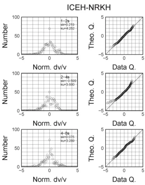
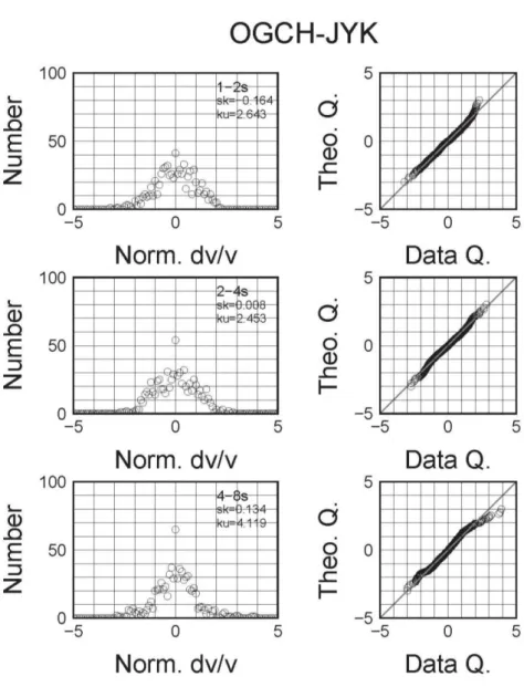
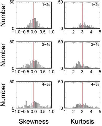
In Figures 5 and 6, we show histograms and normal quantile plots for the 1-2s, 2-4s, and 4-8 second bands of the station pairs ICEH-NRKH and OGCH-JYK in the Iwate-Miyagi data set. Histograms in the left panels show the number of data in each bin with a width of 0.1 from -5 to 5. Data follow symmetric bell shapes. ‘sk’ and ‘ku’ in each panel are skewness and kurtosis of the data. Skewness and kurtosis values are expected to be 0 and 3, respectively, for a Gaussian distribution. On the normal quantile plots in the right panels, data roughly follow straight lines, though data in the 2-4s band of the ICEH-NRKH pair seem slightly convex downward. For the examples shown in Figures 5 and 6, skewness values range from -0.599 to 0.219, including 0, and kurtosis values are from 2.453 to 4.252 sandwiching 3. We show histograms of the skewness and kurtosis values for all station pairs in the Iwate-Miyagi data set in Figure 7. Skewness values are peaked around 0 in the left panel suggesting a symmetric distribution. Kurtosis values are ranging between 2 and 4, not peaked around 3 as expected for the Gaussian. However, normal quantile plots still show almost straight lines. Therefore, we judge that all the results of the Iwate-Miyagi data set obey the Gaussian distribution.
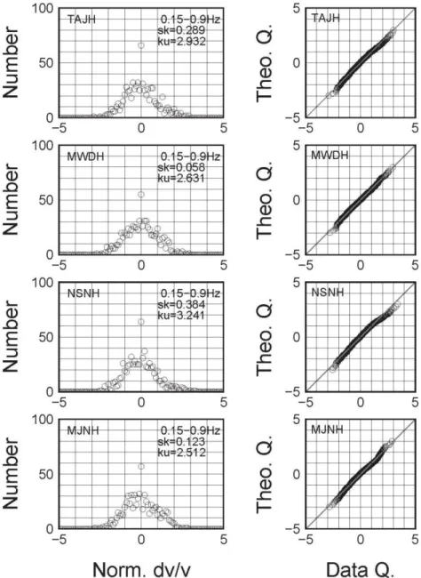
Then, we deal with the second data set: seismic velocity changes in the 0.15-0.9Hz band over the entire Japan. Figure 8 shows the results for four stations. The top three stations belong to the Northeast (NE) Japan group, and the bottom station belongs to the Southwest (SW) Japan group. Left panels show symmetric bell shapes. Right panels exhibit straight lines on the normal quantile plots, which suggests that the Gaussian distribution explains the data. Skewness values for these four stations range from 0.058 to 0.384, slightly higher than 0, and kurtosis values range from 2.512 to 3.241, sandwiching 3. Figure 9 shows skewness and kurtosis values for all stations in the NE Japan group and in the SW Japan group. According to the left panels, skewness values are peaked around 0, suggesting the symmetry of the distributions. The right panels show that kurtosis values are located around 3, suggesting the Gaussian distribution. Therefore, we think that all the results
5 6 7 8 9 10 11 12 13 14 15 16 17 18 19 20 21 22 23 24 25 26 27 28 29 30 31 32 33 34 35 36 37 38 39 40 41 42 43 44 45 46 47 48 49 50 51 52 53 54 55 56 57 58 59 60
10
of the entire Japan data set obey the Gaussian distribution well.
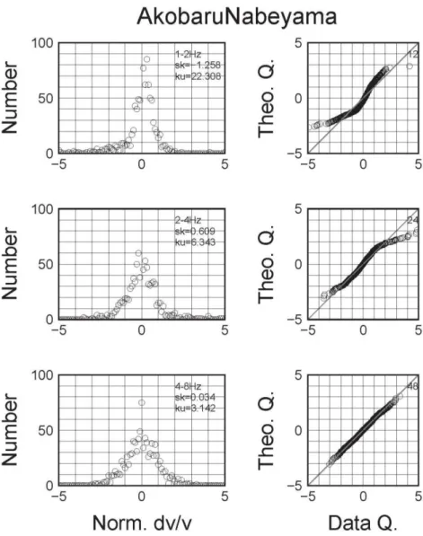
We move on to the last data set for Sakurajima volcano. Figures 10 and 11 show the results for two station pairs in the 1-2, 2-4, and 4-8 Hz bands. Histograms on the left panels are symmetric but with longer tails to both ends. Skewness values are around 0, which suggests the symmetry of the distributions. However, kurtosis values are much larger than 3 in the 1-2 and 2-4 Hz bands. The normal quantile plots on the left panels exhibit apparent deviations from the straight lines in these two lower frequency bands. The shape is like a skewed letter S. These results suggest that more outliers are expected than the Gaussian in the 1-2 Hz and 2-4Hz bands. On the other hand, results in the 4-8Hz band seem to follow the Gaussian. Indeed, skewness values are close to 0, and kurtosis values are close to 3.
To summarize the results, most of the observed seismic velocity changes during normal periods follow the Gaussian distribution. Exceptions are found in the 1-2 and 2-4 Hz bands for Sakurajima. In the next section, we discuss what statistical distribution explains these deviations from the Gaussian and what causes these deviations.
5. Discussions
5.1 Cauchy distribution for the Sakurajima dataset in lower frequencies
In the previous section, we found that the observed seismic velocity changes in the 1-2Hz and 2-4 Hz bands for Sakurajima are not explained by the Gaussian distribution. Here, we discuss what distribution explains these data in a good way. To see the characteristics in more detail, we plot the histograms of the two station pairs shown in Figures 10 and 11 in the log-log scale in Figure 12. In these panels, positive velocity changes are expressed by open circles. For negative velocity changes, absolute values are taken and then plotted by open triangles. In the 1-2Hz and 2-4Hz bands, the
5 6 7 8 9 10 11 12 13 14 15 16 17 18 19 20 21 22 23 24 25 26 27 28 29 30 31 32 33 34 35 36 37 38 39 40 41 42 43 44 45 46 47 48 49 50 51 52 53 54 55 56 57 58 59 60
11
histograms are flat for smaller dv/v values, and then seem to decay linearly in the log-log scale, which suggests that the data follow some power-law like distribution in the tails. On the contrary, the results in the 4-8Hz band are explained by the Gaussian, and the histograms do not show linear decays with the horizontal axis in the log-log scale.
Trying different power-law distributions, we end up with Cauchy distribution C(0, s), whose probability density function p(x) is expressed as
21
( )
,
1
/
p x
s
x s
(5)where s is the scale parameter, and x is a variable that is a daily seismic velocity change in this study. To show its appropriateness, we make random samplings from populations following the Cauchy distribution. The distribution function of Cauchy distribution F(x) is
1
1
1
( )
tan
.
2
x
F x
s
(6)Putting a uniform random number ui between 0 and 1 into the left-hand side of equation (6), we can
reproduce a random number xi following Cauchy distribution as
1
tan
.
2
i ix
s
u
(7)We practically introduce a truncation level xm because there seem upper and lower bounds on real
data. When the absolute value of a sample | xi | exceeds the truncation level, this sample is rejected.
5 6 7 8 9 10 11 12 13 14 15 16 17 18 19 20 21 22 23 24 25 26 27 28 29 30 31 32 33 34 35 36 37 38 39 40 41 42 43 44 45 46 47 48 49 50 51 52 53 54 55 56 57 58 59 60
12
Finally, we superimpose the Cauchy distribution C(0, s) over the standard normal distribution
N(0,1).
1
tan
,
2
i i ix
s
u
r
(8)where ri is a random number sampled from the standard normal distribution N(0,1). An underlying
assumption of this is as follows; Seismic velocity changes generally obey the Gaussian distribution as shown for all the datasets except for the 1-2 and 2-4 Hz bands at Sakurajima. On the other hand, the seismic velocity change in the 1-2Hz and 2-4Hz bands at Sakurajima are contaminated by the Cauchy distribution that is probably due to small-amplitude volcanic earthquakes and tremors. We will discuss this later in this subsection.
Assuming xm =8 and 16, we try four different s values of 0.25, 0.5, 1, and 2. The assumption of xm
does not change shapes of quantile plots seriously. However, larger xm values extend both ends of
the distribution and accordingly increase the kurtosis value. To mimic daily seismic velocity changes for three years at Sakurajima, we randomly sample 1100 data from the population. In Figure 13 (a) and (b), we show histograms for a realization of 1100 samples with eight different combinations of xm and s values. Skewness values are around 0, and kurtosis values get larger than
3 as s becomes smaller, which confirms an apparent deviation from the Gaussian distribution. The cases with smaller s values explain the skewed S letter shape on the normal quantile plots. Therefore, we conclude that the truncated Cauchy distribution superimposing the standard normal distribution well explains the statistical distribution of observed seismic velocity changes for Sakurajima in the 1-2, and 2-4 Hz bands. 5 6 7 8 9 10 11 12 13 14 15 16 17 18 19 20 21 22 23 24 25 26 27 28 29 30 31 32 33 34 35 36 37 38 39 40 41 42 43 44 45 46 47 48 49 50 51 52 53 54 55 56 57 58 59 60
13
Now, we discuss why only the results in the lower frequencies at Sakurajima show clear deviations from the Gaussian. We compare dates of outliers in observed seismic velocity changes with days of heavy rainfall by checking precipitation data, but we cannot find the significant correspondence. Predominant frequencies of volcanic tremors at Sakurajima are known to be between 1.3 and 3Hz (Iguchi, 2013). We now speculate as follows: Tiny signals from volcanic earthquakes and tremors are hidden in ambient seismic noise and might affect the estimation of seismic velocity changes by contaminating the noise wavefield. The Japan Meteorological Agency (JMA) reported activities of volcanic earthquakes and tremor at Sakurajima between 2012 and 2014. Then, we make the normal quantile plots of data on the days (154 days between 2012 and 2014) when no volcanic tremors were identified by JMA, and show them in Figures 14 and 15. The data actually get closer to the Gaussian though some disagreements still remain especially for station pair Amidagawa-Yuno station pair.
5.2 Contributions from known physical components
In the results section, we show that most of the observed seismic velocity changes obey a Gaussian distribution with exceptions of the low-frequency bands at Sakurajima. Based on the central limit theorem, we might interpret that several competing factors contribute to the observed seismic velocity changes. However, in some cases, one or two predominant factors such as pore pressure change induced by precipitation and elastic loading change generated by snow accumulation and sea height variation can affect the observed seismic velocity changes (Wang et al., 2017). In this section, we show examples of how a fit to a Gaussian distribution is improved by subtracting contributions of dominant factors from the observed seismic velocity changes in different regions in Japan following the study by Wang et al. (2017).
In Figure 8, we have shown that the results in 0.15-0.9 Hz at four stations almost obey the Gaussian
5 6 7 8 9 10 11 12 13 14 15 16 17 18 19 20 21 22 23 24 25 26 27 28 29 30 31 32 33 34 35 36 37 38 39 40 41 42 43 44 45 46 47 48 49 50 51 52 53 54 55 56 57 58 59 60
14
distribution. In order to see the improvement in Gaussian fit by removing the external forcing-generated changes, we start with the station NSNH, which is relatively less normal distributed compared with others. We make quantile plots of the data and calculate the skewness and kurtosis values in Figure 16. The results show that after subtracting the synthetic velocity changes from the physical model, the skewness changes from 0.384 to 0.275 and the kurtosis changes from 3.241 to 3.199. Both parameters slightly get closer to 0 and 3, respectively. Then we try with the other three stations TREH, ARKH, and UWEH, which are the same as in Figure 10 by Wang et al. (2017). They discussed that those stations had been strongly affected by some local external forcing. Globally, we confirm from the values of skewness and kurtosis before and after the physical model correction that the Gaussian fit has been improved after correction.
Finally, we check the changes in skewness and kurtosis for all stations throughout Japan using dv/v measured from 2009 to 2010 in the Northeast and from 2011 to 2012 in Southwest Japan in Figure 17. The two groups of histograms present how the two values systematically change before and after applying the physical model correction. We can see that skewness and kurtosis get more concentrated around 0 and 3, respectively. This observation confirms that the physical model-based seismic velocity correction can help remove some non-random portion of changes in seismic velocity. Applying the physical model correction can further help sort better changes in seismic velocity that related to long-term tectonic deformations and better quantitatively summarize the probability of seismic velocity changes.
5.3 Applications of the statistical distributions
Here we discuss some applications of the statistical distributions of observed seismic velocity changes. The discussion in the previous section will help to check if we can correctly remove contributions of known physical mechanisms to the observed seismic velocity changes based on their Gaussianities. That is one practical application of what we found in this study. Moreover,
5 6 7 8 9 10 11 12 13 14 15 16 17 18 19 20 21 22 23 24 25 26 27 28 29 30 31 32 33 34 35 36 37 38 39 40 41 42 43 44 45 46 47 48 49 50 51 52 53 54 55 56 57 58 59 60
15
another application is the quantification of anomalies by using probabilities. Once we know that observed seismic velocity changes statistically obey Gaussian distribution, we can assign a probability to each daily seismic velocity change. Then we can quantitatively judge if a current seismic velocity change is normal or abnormal. Figure 18 is similar to Figure 3, but the vertical axis is the seismic velocity change normalized by its standard deviation during the normal period. Red horizontal lines show +/- four times the standard deviation. According to the Gaussian distribution, a probability of exceeding +/- four times the standard deviation is only about 10^-4 (0.01%). Therefore, we can quantify how often a seismic velocity change exceeds this threshold with this probability. If the seismic velocity change exceeds the threshold for two successive days, the probability becomes as low as 10^-8. In the top three panels, seismic velocity changes exceed -4 times the standard deviation associated with the Tohoku-Oki earthquake on March 11, 2011. According to the results, we can quantitatively evaluate how rare such a large seismic velocity change is. Such quantification also helps monitor seismic velocity changes and detect some anomalies automatically without human intervention.
6. Conclusions
We have investigated statistical distributions of seismic velocity changes observed during normal periods when no large earthquakes or volcanic eruptions are known to occur by analyzing three different data sets of seismic velocities measured in Japan. Results show that the Gaussian distribution well explains most of the observed seismic velocity changes. However, an exception is the superposition of the truncated Cauchy distribution over the Gaussian distribution that well describes the results for the 1-2 and 2-4 Hz frequency bands at Sakurajima volcano. The truncated Cauchy distribution is a power-law like distribution which has longer tails than the Gaussian distribution. Reasons for such an exception are still open, but we speculate that small-amplitude volcanic earthquakes and tremors at Sakurajima might change the seismic noise wavefield, and accordingly affect the estimation of seismic velocity changes. Once the statistical distribution is
5 6 7 8 9 10 11 12 13 14 15 16 17 18 19 20 21 22 23 24 25 26 27 28 29 30 31 32 33 34 35 36 37 38 39 40 41 42 43 44 45 46 47 48 49 50 51 52 53 54 55 56 57 58 59 60
16
known, either Gaussian or the other, we can assign a probability to a current value of the observed daily seismic velocity change. Accordingly, we can objectively judge if the current value is normal or abnormal based on the probability. The statistical distribution of seismic velocity changes can be utilized to quantify the monitoring of seismic velocity changes using probabilities. Furthermore, such quantitative monitoring is useful for automatic detections of anomalies in seismic velocity changes without human intervention.
Acknowledgments
We used daily numbers of volcanic tremors at Sakurajima identified by the Japan Meteorological Agency. This collaborative study was realized thanks to the continuous support from our colleagues and friends: Drs. Michel Campillo and Florent Brenguier at Institut des Sciences de la Terre, Université Grenoble Alpes, France, Drs. Haruo Sato and Takeshi Nishimura at Tohoku University, Japan, Dr. Ulrich Wegler at Friedrich-Schiller-Universität Jena, Germany, and Dr. Katsuhiko Shiomi at National Research Institute for Earth Science and Disaster Resilience, Japan. This study was partially supported by the Japan Society for the Promotion of Science (JSPS) KAKENHI Grant 16K05528. Qing-Yu Wang acknowledges the funding from the European Research Council (ERC) under the European Union Horizon 2020 Research and Innovation Program (Grant Agreement 742335, F-IMAGE). 5 6 7 8 9 10 11 12 13 14 15 16 17 18 19 20 21 22 23 24 25 26 27 28 29 30 31 32 33 34 35 36 37 38 39 40 41 42 43 44 45 46 47 48 49 50 51 52 53 54 55 56 57 58 59 60
17
References
Bensen, G. D., M. H. Ritzwoller, M.P. Barmin, A. L. Levshin, F. Lin, M. P. Moschetti, N.M. Shapiro, & Y. Yang, 2007, Processing seismic ambient noise data to obtain reliable broad-band surface wave dispersion measurements, Geophys. J. Int., 169(3), 1239-1260.
Brenguier, F., M. Campillo, C. Hadziioannou, N. M. Shapiro, R. M. Nadeau, and E. Larose, 2008a, Postseismic relaxation along the San Andreas fault at Parkfield from continuous seismological observations, Science, 321, 1478-1481.
Brenguier, F., N. M. Shapiro, M. Campillo, V. Ferrazzini, Z. Duputel, O. Coutant, and A. Nercessian, 2008b, Towards forecasting volcanic eruptions using seismic noise, Nature Geoscience,
1, 126-130, doi:10.1038/ngeo104.
Brenguier, F., M. Campillo, T. Takeda, Y. Aoki, N. M., Shapiro, X. Briand, K. Emoto, and H. Miyake, 2014, Mapping pressurized volcanic fluids from induced crustal seismic velocity drops, Science, 345(6192), 80-82.
Campillo, M. & Paul, A., 2003, Long-range correlations in the diffuse seismic coda, Science,
299(5606), 547-549.
Curtis, A., Gerstoft, P, Sato, H., Snieder, R., & Wapenaar, K., 2006, Seismic interferometry- turning noise into signal, The leading edge, 25, 1082-1092.
Hirose, T., H. Nakahara, & T. Nishimura, 2017, Combined use of repeated active shots and ambient noise to detect temporal changes in seismic velocity: application to Sakurajima volcano, Japan, Earth Planets and Space, 69, .
5 6 7 8 9 10 11 12 13 14 15 16 17 18 19 20 21 22 23 24 25 26 27 28 29 30 31 32 33 34 35 36 37 38 39 40 41 42 43 44 45 46 47 48 49 50 51 52 53 54 55 56 57 58 59 60
18
Hobiger, M., Wegler, U., Shiomi, K., & Nakahara, H., 2012, Coseismic and postseismic elastic wave velocity variations caused by the 2008 Iwate-Miyagi Nairiku earthquake, Japan, J. Geophys. Res., 117, B09313, doi:10.1029/2012jb009402 .
Iguchi, M., 2013, A method for monitoring of discharge volume of volcanic ash by using volcanic tremor, Annuals of Disas. Prev. Res. Inst. Kyoto Univ., 56B, 221-225.
Li, Y. G., J. E. Vidale, K. Aki, F. Xu, and T. Burdette, 1998, Evidence of shallow fault zone strengthening after the 1992 M7.5 Landers, California, earthquake, Science, 279, 217-219.
Meier, U., N. M. Shapiro, and F. Brenguier, 2010, Detecting seasonal variations in seismic velocities within Los Angeles basin from correlations of ambient seismic noise, Geophys. J. Int., 181, 985-996.
Nishimura, T., S. Tanaka, T. Yamawaki, H. Yamamoto, T. Sano, M. Sato, H. Nakahara, N. Uchida, S. Hori, and H. Sato, 2005, Temporal changes in seismic velocity of the crust around Iwate volcano, Japan, as inferred from analyses of repeated active seismic experiment data, Earth Planets Space, 57, 491-505.
Pacheco, C., & Snieder, R., 2005, Time-lapse travel time change of multiply scattered acoustic waves, J. Acoust. Soc. Am., 118(3), 1300-1310.
Pacheco, C., & Snieder, R., 2006, Time-lapse traveltime change of singly scattered acoustic waves, Geophys. J. Int., 165(2), 485-500. 5 6 7 8 9 10 11 12 13 14 15 16 17 18 19 20 21 22 23 24 25 26 27 28 29 30 31 32 33 34 35 36 37 38 39 40 41 42 43 44 45 46 47 48 49 50 51 52 53 54 55 56 57 58 59 60
19
Poupinet, G., W. L. Ellsworth, and J. Frechet (1984), Monitoring velocity variations in the crust using earthquake doublets: an application to the Calaveras fault, California, J. Geophys. Res., 89, 5719-5731.
Sato, H., Fehler, M. C., & Maeda, T., 2012, Seismic wave propagation and scattering in the
heterogeneous Earth, 2nd edition, Springer, Berlin.
Sens-Schöfelder, C. & U. Wegler, 2006, Passive image interferometry and seasonal variations of seismic velocities at Merapi Volcano, Indonesia, Geophys. Res. Lett., 33(21).
Sens-Schönfelder, C., and U. Wegler, 2011, Passive image interferometry for monitoring crustal changes with ambient seismic noise, Comptes Rendus Geoscience, 343, 639-651.
Shapiro, N. M., and M. Campillo (2004), Emergence of broadband Rayleigh waves from correlations of the ambient seismic noise, Geophys. Res. Lett., 31, L07614, doi:
10.1029/2004GL019491.
Wang, Q. Y., F. Brenguier, M. Campillo, A. Lecointre, T. Takeda, and Y. Aoki, 2017, Seasonal Crustal Seismic Velocity Changes Throughout Japan, J. Geophys. Res. Solid Earth, 122(10), 7987-8002.
Wegler, U., H. Nakahara, C. Sens-Schönfelder, M. Korn, and K. Shiomi, 2009, Sudden drop of seismic velocity after the 2004 Mw6.6 Mid-Niigata earthquake, Japan, observed with Passive Image Interferometry, J. Geophys. Res., 114, B06305, doi:10.1029/2008JB005869.
5 6 7 8 9 10 11 12 13 14 15 16 17 18 19 20 21 22 23 24 25 26 27 28 29 30 31 32 33 34 35 36 37 38 39 40 41 42 43 44 45 46 47 48 49 50 51 52 53 54 55 56 57 58 59 60
20
Wegler, U., and C. Sens-Schönfelder, 2007, Fault zone monitoring with passive image interferometry, Geophys. J. Int., 168, 1029-1033, doi: 10.1111/j.1365-246X.2006.03284.x.
Wessel, P. and W. H. F. Smith (1998), New improved version of the Generic Mapping Tools released, EOS Trans., Am. Geophys. Union, 79, 579.
5 6 7 8 9 10 11 12 13 14 15 16 17 18 19 20 21 22 23 24 25 26 27 28 29 30 31 32 33 34 35 36 37 38 39 40 41 42 43 44 45 46 47 48 49 50 51 52 53 54 55 56 57 58 59 60
21
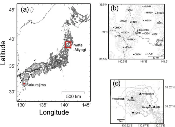
Figure 1 Maps of the study areas for three different data sets of observed seismic velocity changes. (a) All over Japan for Wang et al. (2017). Gray squares show stations in Northeastern Japan, and open triangles are those in Southwestern Japan. Red rectangles are areas zoomed up in (b) and (c). (b) Source area of the 2008 Iwate-Miyagi Nairiku earthquake. A solid star is the epicenter, and solid triangles are stations used in Hobiger et al. (2012). Thick broken curves are prefectural boundaries, and gray contours show elevations with an interval of 250m. (c)
Sakurajima volcano. Solid triangles are six stations used in Hirose et al. (2017). Contours show the topography of the volcano.
5 6 7 8 9 10 11 12 13 14 15 16 17 18 19 20 21 22 23 24 25 26 27 28 29 30 31 32 33 34 35 36 37 38 39 40 41 42 43 44 45 46 47 48 49 50 51 52 53 54 55 56 57 58 59 60
22
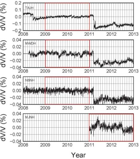
Figure 2 Examples of seismic velocity changes measured in the source area of the 2008 Iwate-Miyagi Nairiku earthquake between 2008 to the middle of 2011. The left panels are results for a station pair ICEH-NRKH in the 1-2s, 2-4s, and 4-8s from top to bottom. The right panels are those for OGCH-JYK. Sudden drops in the middle of 2008 and early 2011 correspond to the changes associated with the June 14, 2008 Iwate-Miyagi Nairiku earthquake and those with the March 11, 2011 Tohoku-Oki earthquake, respectively. Two years of 2009 and 2010 enclosed by a red rectangle are selected for the normal period when no large earthquakes took place.
5 6 7 8 9 10 11 12 13 14 15 16 17 18 19 20 21 22 23 24 25 26 27 28 29 30 31 32 33 34 35 36 37 38 39 40 41 42 43 44 45 46 47 48 49 50 51 52 53 54 55 56 57 58 59 60
23
Figure 3 Examples of seismic velocity changes measured all over Japan from 2008 to 2012. The top three panels show results obtained at three stations in Northeast Japan, and the bottom panel shows results at one station in Southwest Japan. In the top three panels, we can recognize two sudden velocity drops associated with the Iwate-Miyagi Nairiku earthquake in June 2008 and the Tohoku-Oki earthquake on March 11, 2011. We choose the years 2009 and 2010 as the normal period for Northeast Japan, and the years 2011 and 2012 as the normal period for Southwest Japan. These normal periods are enclosed by red rectangles.
5 6 7 8 9 10 11 12 13 14 15 16 17 18 19 20 21 22 23 24 25 26 27 28 29 30 31 32 33 34 35 36 37 38 39 40 41 42 43 44 45 46 47 48 49 50 51 52 53 54 55 56 57 58 59 60
24
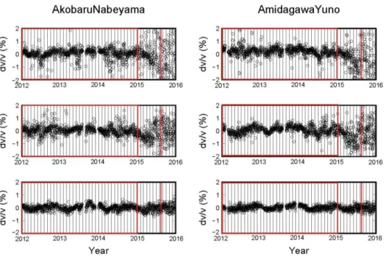
Figure 4 Examples of seismic velocity changes measured at Sakurajima from 2012 to 2015. The left panels are results for station pair Akobaru-Nabeyama in the 1-2, 2-4, and 4-8Hz bands from top to bottom. The right panels are those for Amidagawa-Yuno. The red vertical lines indicate August 15, 2015 when a dike intrusion event took place. We choose the years 2012, 2013, and 2014 enclosed by a red rectangle as the normal period
5 6 7 8 9 10 11 12 13 14 15 16 17 18 19 20 21 22 23 24 25 26 27 28 29 30 31 32 33 34 35 36 37 38 39 40 41 42 43 44 45 46 47 48 49 50 51 52 53 54 55 56 57 58 59 60
25
Figure 5 Histograms (left) and normal quantile plots (right) for the 1-2s, 2-4s, and 4-8 second bands (from top to bottom) for the station pair ICEH-NRKH for the Iwate-Miyagi data set. In each panel on the left, ‘sk’ and ‘ku’ stand for skewness and kurtosis of the data. In each panel on the right, a one-to-one line is shown by a solid line.
5 6 7 8 9 10 11 12 13 14 15 16 17 18 19 20 21 22 23 24 25 26 27 28 29 30 31 32 33 34 35 36 37 38 39 40 41 42 43 44 45 46 47 48 49 50 51 52 53 54 55 56 57 58 59 60
26
Figure 6 Histograms (left) and normal quantile plots (right) for the 1-2s, 2-4s, and 4-8 second bands (from top to bottom) for station pair OGCH-JYK for the Iwate-Miyagi data set. In each panel on the left, ‘sk’ and ‘ku’ stand for skewness and kurtosis of the data. In each panel on the right, a one-to-one line is shown by a solid line.
5 6 7 8 9 10 11 12 13 14 15 16 17 18 19 20 21 22 23 24 25 26 27 28 29 30 31 32 33 34 35 36 37 38 39 40 41 42 43 44 45 46 47 48 49 50 51 52 53 54 55 56 57 58 59 60
27
Figure 7 Skewness (left) and kurtosis (right) values for all 190 station pairs of the Iwate-Miyagi data set in the 1-2s, 2-4s, and 4-8s period bands. Vertical lines in the left panels indicate 0, the expected skewness for the Gaussian distribution. Vertical lines in the right panels correspond to 3, the expected kurtosis for the Gaussian distribution.
5 6 7 8 9 10 11 12 13 14 15 16 17 18 19 20 21 22 23 24 25 26 27 28 29 30 31 32 33 34 35 36 37 38 39 40 41 42 43 44 45 46 47 48 49 50 51 52 53 54 55 56 57 58 59 60
28
Figure 8 Histograms (left) and normal quantile plots (right) for four stations for the entire Japan data set. In each panel on the left, ‘sk’ and ‘ku’ stand for skewness and kurtosis of the data. In each panel on the right, a one-to-to line is shown by a solid line.
5 6 7 8 9 10 11 12 13 14 15 16 17 18 19 20 21 22 23 24 25 26 27 28 29 30 31 32 33 34 35 36 37 38 39 40 41 42 43 44 45 46 47 48 49 50 51 52 53 54 55 56 57 58 59 60
29
Figure 9 Skewness (left) and kurtosis (right) values for all stations in Southwest Japan (top) and Northeast Japan (bottom) of the entire Japan data set. Vertical lines in the left panels indicate 0, the expected skewness for the Gaussian distribution. Vertical lines in the right panels correspond to 3, the expected kurtosis for the Gaussian distribution.
5 6 7 8 9 10 11 12 13 14 15 16 17 18 19 20 21 22 23 24 25 26 27 28 29 30 31 32 33 34 35 36 37 38 39 40 41 42 43 44 45 46 47 48 49 50 51 52 53 54 55 56 57 58 59 60
30
Figure 10 Histograms (left) and normal quantile plots (right) for the 1-2Hz, 2-4Hz, and 4-8 Hz bands (from top to bottom) for the station pair Akobaru-Nabeyama for the Sakurajima data set. In each panel on the left, ‘sk’ and ‘ku’ stand for skewness and kurtosis of the data. In each panel on the right, a one-to-one line is shown by a solid line.
5 6 7 8 9 10 11 12 13 14 15 16 17 18 19 20 21 22 23 24 25 26 27 28 29 30 31 32 33 34 35 36 37 38 39 40 41 42 43 44 45 46 47 48 49 50 51 52 53 54 55 56 57 58 59 60
31
Figure 11 Histograms (left) and normal quantile plots (right) for the 1-2Hz, 2-4Hz, and 4-8 Hz bands (from top to bottom) for the station pair Amidagawa-Yuno for the Sakurajima data set. In each panel on the left, ‘sk’ and ‘ku’ stand for skewness and kurtosis of the data. In each panel on the right, a one-to-one line is shown by a solid line.
5 6 7 8 9 10 11 12 13 14 15 16 17 18 19 20 21 22 23 24 25 26 27 28 29 30 31 32 33 34 35 36 37 38 39 40 41 42 43 44 45 46 47 48 49 50 51 52 53 54 55 56 57 58 59 60
32
Figure 12 Histograms in the log-log scale for the 1-2Hz, 2-4Hz, and 4-8 Hz bands (from top to bottom) for the station pairs Akobaru-Nabeyama (left) and Amidagawa-Yuno (right) for the Sakurajima data set. In each panel, positive values of seismic velocity changes are shown by open circles and for negative values, their absolute values are taken and shown by open triangles.
5 6 7 8 9 10 11 12 13 14 15 16 17 18 19 20 21 22 23 24 25 26 27 28 29 30 31 32 33 34 35 36 37 38 39 40 41 42 43 44 45 46 47 48 49 50 51 52 53 54 55 56 57 58 59 60
33
Figure 13 (a) Histograms (left) and normal quantile plots (right) for a realization of 1100 samples from the population following Cauchy distribution with the truncation level xm of 8 for four
different s values. In each panel on the left, ‘sk’ and ‘ku’ stand for skewness and kurtosis of the data. In each panel on the right, a one-to-one line is shown by a solid line.
5 6 7 8 9 10 11 12 13 14 15 16 17 18 19 20 21 22 23 24 25 26 27 28 29 30 31 32 33 34 35 36 37 38 39 40 41 42 43 44 45 46 47 48 49 50 51 52 53 54 55 56 57 58 59 60
34
Figure 13 (b) Histograms (left) and normal quantile plots (right) for a realization of 1100 samples from the population following Cauchy distribution with the truncation level xm of 16 for four
different s values. In each panel on the left, ‘sk’ and ‘ku’ stand for skewness and kurtosis of the data. In each panel on the right, a one-to-one line is shown by a solid line.
5 6 7 8 9 10 11 12 13 14 15 16 17 18 19 20 21 22 23 24 25 26 27 28 29 30 31 32 33 34 35 36 37 38 39 40 41 42 43 44 45 46 47 48 49 50 51 52 53 54 55 56 57 58 59 60
35
Figure 14 Histograms (left) and normal quantile plots (right) for the 1-2Hz, 2-4Hz, and 4-8 Hz bands (from top to bottom) for the station pair Akobaru-Nabeyama only for the days when no volcanic tremors were identified. In each panel on the left, ‘sk’ and ‘ku’ stand for skewness and kurtosis of the data. In each panel on the right, a one-to-to line is shown by a solid line.
5 6 7 8 9 10 11 12 13 14 15 16 17 18 19 20 21 22 23 24 25 26 27 28 29 30 31 32 33 34 35 36 37 38 39 40 41 42 43 44 45 46 47 48 49 50 51 52 53 54 55 56 57 58 59 60
36
Figure 15 Histograms (left) and normal quantile plots (right) for the 1-2Hz, 2-4Hz, and 4-8 Hz bands (from top to bottom) for the station pair Amidagawa-Yuno only for the days when no volcanic tremors were identified. In each panel on the left, ‘sk’ and ‘ku’ stand for skewness and kurtosis of the data. In each panel on the right, a one-to-one line is shown by a solid line.
5 6 7 8 9 10 11 12 13 14 15 16 17 18 19 20 21 22 23 24 25 26 27 28 29 30 31 32 33 34 35 36 37 38 39 40 41 42 43 44 45 46 47 48 49 50 51 52 53 54 55 56 57 58 59 60
37
Figure 16 Histograms (left) and normal quantile plots (right) for four stations for the entire Japan data set but with the external forcing-generated changes removed. In each panel on the left, ‘sk’ and ‘ku’ stand for skewness and kurtosis of the data. In each panel on the right, a one-to-one line is shown by a solid line.
5 6 7 8 9 10 11 12 13 14 15 16 17 18 19 20 21 22 23 24 25 26 27 28 29 30 31 32 33 34 35 36 37 38 39 40 41 42 43 44 45 46 47 48 49 50 51 52 53 54 55 56 57 58 59 60
38
Figure 17 Skewness (left) and kurtosis (right) values for all stations in Southwest Japan (top) and Northeast Japan (bottom) of the entire Japan data set. Blue and red show the results for the data before and after the correction of the external forcing-generated changes, respectively. Vertical lines in the left panels indicate 0, the expected skewness for the Gaussian distribution. Vertical lines in the right panels correspond to 3, the expected kurtosis for the Gaussian distribution.
5 6 7 8 9 10 11 12 13 14 15 16 17 18 19 20 21 22 23 24 25 26 27 28 29 30 31 32 33 34 35 36 37 38 39 40 41 42 43 44 45 46 47 48 49 50 51 52 53 54 55 56 57 58 59 60
39
Figure 18 Examples of seismic velocity changes measured all over Japan from 2008 to 2012. The vertical axis means the seismic velocity change normalized by its standard deviation during the normal period. The top three panels show results obtained at three stations in Northeast Japan, and the bottom panel shows results at one station in Southwest Japan. The horizontal red lines show +/- 4 standard deviation as a threshold level to detect anomalies.
5 6 7 8 9 10 11 12 13 14 15 16 17 18 19 20 21 22 23 24 25 26 27 28 29 30 31 32 33 34 35 36 37 38 39 40 41 42 43 44 45 46 47 48 49 50 51 52 53 54 55 56 57 58 59 60