HAL Id: hal-00647485
https://hal.archives-ouvertes.fr/hal-00647485
Submitted on 2 Dec 2011
HAL is a multi-disciplinary open access
archive for the deposit and dissemination of
sci-entific research documents, whether they are
pub-lished or not. The documents may come from
teaching and research institutions in France or
abroad, or from public or private research centers.
L’archive ouverte pluridisciplinaire HAL, est
destinée au dépôt et à la diffusion de documents
scientifiques de niveau recherche, publiés ou non,
émanant des établissements d’enseignement et de
recherche français ou étrangers, des laboratoires
publics ou privés.
RFI mitigation: cyclostationary criterion
Rym Feliachi, Cedric Dumez-Viou, Rodolphe Weber, Albert-Jan Boonstra
To cite this version:
Rym Feliachi, Cedric Dumez-Viou, Rodolphe Weber, Albert-Jan Boonstra. RFI mitigation:
cyclo-stationary criterion. S. A. Torchinsky, A. van Ardenne, T. van den Brink-Havinga, A. van Es, A.J.
Faulkner. Widefield Science and Technology for the SKA SKADS Conference 2009, ISBN
978-90-805434-5-4, pp.201 - 205, 2010, ISBN 978-90-805434-5-4. �hal-00647485�
Abstract.Radio astronomical observations are increasingly corrupted by radio frequency interferences. Thus, real-time filtering algorithms are becoming essential. One approach is to use a specific real-time property of the Telecoms signals : the cyclostationarity. This property can be exploited for detection purpose or filtering purpose. In par-ticular, new generations of radio telescopes will be based on antenna arrays providing the possibility of applying spatial filtering techniques. In this paper, we compare the performance between classical approaches based on power statistics and cyclic approaches. This comparison is done through simulations on synthetic data and through simulations on real data acquired with the new generation low frequency array radio telescope, LOFAR.
1. Introduction
For several years, radio astronomy has had to face two contradictory trends. On the one hand, the exponential expansion of telecommunications has generated a growing demand on the electromagnetic spectrum, reducing the bandwidths available for good quality radio astronomical observations. On the other hand, radio astronomical needs in terms of sensitivity and bandwidth have also grown. As a result, radio frequency interference (RFI) mitigation has become a significant issue for current and future radio tele-scopes. The various methods that have been tried to limit RFI depend on the type of interference and the type of in-struments. Time, frequency and/or spatial properties can be considered in order to find efficient excision processing techniques, see for example the inventory carries out in the framework of SKADS DS4T3 work package (2009).
Most communication signals contain recurrent char-acteristics which stem, for example, from a transmitter carrier frequency or from a communication signal baud rate. Usually, these periodicities are scrambled and hid-den by the intrinsic signal randomness. However, to some extent, these periodicities can be regenerated. If it is the case, such signals are so called cyclostationary signals, or in short, cyclic signals. This specific property can be used to discriminate them from natural signals.
2. What is the cyclostationarity ?
Mathematically, a cyclostationary process means that its statistics are periodic with time. For example, let us con-sider the second order statistics given by the correlation of a given process x(t):
R(t, τ ) = E{x(t − τ2)x(t +τ
2)} (1)
where E{.} represents the ensemble average operator. If the process is modeled as stationary then R(t, τ ) = R(τ ). If the process is modeled as cyclostationary then
∃T/R(t + T, τ) = R(t, τ). T is called the cyclic pe-riod. Review papers on cyclostationarity can be found in Gardner (2006) or Serpedin(2005).
To illustrate these concepts, let us consider the fol-lowing simple baseband signal, x(t) =Pk∈Zakg(t − kT ),
where akis a random digital message with power σa2, g(t),
its pulse shape and T , its baud rate. The correlation of x(t) becomes :
R(t, τ ) = σa2
X
k∈Z
g(t − kT +τ2)g(t − kT −τ2) (2) One can easily verify that R(t, τ ) is T -periodic. So, it can be decomposed in Fourier series and the corresponding Fourier coefficients are (k ∈ Z):
Rα=k T(τ ) =σ 2 a T Z +∞ −∞ g(t +τ 2)g(t − τ 2) exp(−j2παt)dt | {z } rα g(τ ) (3)
In practice, a time average approach is preferred and Rα
(τ ), also called the cyclic correlation, is given by:
Rα(τ ) = lim N→+∞ 1 N Z N x(t +τ 2)x(t − τ 2) exp(−j2παt)dt(4) If Rα
(τ ) is non-zero for some cyclic frequencies, α, with α 6= 0, then x(t) can be modeled as cyclostationary. Note that for α = 0, we retrieve the expression of the classical correlation. Figure 1 gives the plots of these previous ex-pressions for the considered example with a rectangular pulse function.
In the cyclostationary case, the temporal periodicity of the correlation can be exploited to extract RFI infor-mation from the noise. In the next two sections, two RFI mitigation techniques based on the exploitation of the cy-clostationarity are presented.
R. Feliachi et al.: RFI mitigation: cyclostationary criterion
Fig. 1. Random binary signal, x(t) = Pk∈Zakg(t − kT )
with g(t) rectangular. (a) Temporal view. (b) correlation of x(t). R(t, τ ) is T -periodic. (c) the cyclic correlation Rα
(τ ). Rα
(τ ) 6= 0 for α = k
T, k ∈ Z. A stationary process will provide
information only at α = 0.
3. Example of cyclostationary detection
We suppose now that x(t) is a mix of a stationary signal (i.e. a cosmic source and/or the system noise) and a cyclo-stationary signal (i.e. a RFI). Let us consider the following criterion: Cα N = 1 N N−1 X n=0 |x|2(n) exp(−j2παn) (5)
This criterion is just derived from the cyclic correlation defined in Eq. 4 by considering 1) discrete samples and 2) a finite averaging 3) for τ = 0. Actually, through this criterion, we are just looking for periodicities in the in-stantaneous power fluctuations. To make this detector ro-bust again slow power variations, we define a normalized version of our previous criterion:
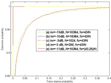
Dα N = √ N Cα N C0 N (6) In Weber (2007), the statistical properties of this de-tector have been derived as a function of the interference to noise ratio. Figure 2 plots the results obtained with an AM signal. If the expected cyclic frequency is not known, a blind cyclostationary detection can be perform by Fourier transform of the instantaneous power. Once spectral lines are detected at non-zero frequencies, it is the signature of a cyclostationary signal.
From that consideration, an operational cyclic detec-tor has been implemented on a real time digital back-end at Nan¸cay Observatory. The backback-end is described in Figure 3.a. The algorithm is implemented into a digital programmable component Virtex II, a FPGA from the Xilinx company. The successive steps are:
1. Channelization of the signal coming from the radio telescope. The signal in each channel is supposed to be complex. This process is done in real time by the digital receiver.
Fig. 2. Probability of detection vs. probability of false alarm for the cyclostationary detector (Eq. 6). The RFI is an AM modulation. Its carrier frequency is fo and the corresponding
expected cyclic frequency is α = 2fo. This simulation is based
on 10000 runs. In cases (a) to (d), fo is chosen so that 2fo is
multiple of 1/N (i.e. the 2fo spectral line is in the middle of
the N bin FFT channel, no attenuation). In case (e), the 2f0
spectral line is between two N bin FFT channels, which is the worst case. The channel attenuation at Nyquist frequency for a rectangular window is ≈ 2 dB. Thus, (e) should be similar to (a).
2. To reduce the computational load of the cyclic de-tector, the algorithm is applied to the real part only (sr(n)) of the signal.We compute the Fourier
trans-form, F F Tm
N(f ), over N samples on s 2
r(n) for the m th
channel, m = 1, . . . , M . M is the number of channels. 3. According to a given threshold ξ derived from the the-oretical study, we will consider that a RFI is present on the mth channel if: ∃k > 0/ √N |F F Tm N(k)| F F Tr N(0) ≥ ξ with ξ =p−2 log(pfa) (7)
where pfa is the expected probability of false alarm. Figure 3.b shows some results obtained in the decame-ter band. In the next section, the cyclostationary concept will be extended to correlation matrices by considering radio telescope arrays.
4. Example of cyclostationary spatial processing
Consider a telescope array consisting of p antennas, each having a received signal xk(t), k = 1, . . . p (see Figure 4.a).
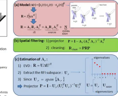
It is assumed that the narrowband condition holds and that geometric delays for each antenna and each impinging source can be represented by phase shifts. In this case, the telescope correlation matrix R can be modeled as:
R = E{xxH } = ArRrA H r + AsRsA H s + N (8)
Fig. 3. a) The current functionalities of the digital system are high dynamic range of 70 dB, bandwidth selection facil-ities ranging from 875 kHz to 14 MHz, high spectral resolu-tion through a polyphase filter bank with up to 8192 channels with 49152 coefficients. A more complete description can be found in Weber (2005) b) Results obtained in the decameter band. The total bandwidth is 7 MHz. The number of channels is M = 2048. On each channel, N = 2048 samples are used to compute the criterion. The cyclic detector is robust against power fluctuations generated by the successive calibration noise diode pulses added to the signal.
where (.)H
is the conjugate transpose operator, Rr is
the Kr × Kr correlation matrix due to the Kr
α-cyclostationary sources (i.e. the RFI), Rsis the Ks× Ks
correlation matrix due to the Ksothers sources (i.e.
sta-tionary sources and non α-cyclostasta-tionary RFI if any) and Nis the p × p correlation matrix due to the system noise. These matrices contain the signal information. Matrices Ar ( p × Kr) and As( p × Ks) contain the spatial
signa-tures of the impinging sources.
In order to remove RFI from the received data, we can filter them out by applying a spatial null in the direction of the undesired signals. Each received signal is identified by its spatial signature in the received data model. If the information contained in Ar can be estimated, then the
RFI can be filtered out (see Figure 4.b).
The proposed estimation method is based on subspace decomposition. If the cosmic sources are negligible and the system noise is calibrated (i.e. R ≈ ArRrAHr + σ2Iwhere
Iis the identity matrix and σ2 the system noise power ), Boonstra (2005) has demonstrated that a close estimate of the information contained in Arcan be derived from the
eigenvalue decomposition (EVD) of R (see Figure 4.c). The same idea can be applied on the cyclic correlation matrix defined by either its ensemble average version or its time average version
Rα= E{R(t) exp(−2παt} (9) Rα= lim N→+∞ 1 N Z N x(t)xH(t) exp(−j2παt)dt (10)
Fig. 4. a) The data array model: The correlation matri-ces Rr, Rsand N contain the signal information. Matrices Ar
and Ascontain the spatial signatures of the impinging sources.
b) Spatial filtering: This method is based on the estimation of the RFI spatial signature vector,Ar, from the correlation
matrix, R followed by a subspace projection to remove that dimension from the correlation matrix, R. To preserve the in-tegrity of the cosmic information, AsRsA
H
r , a correction
ma-trix must be applied on the cleaned correlation mama-trix, Rclean (see Boonstra (2005)). c) Estimation of Ar: the signal
sub-space, Ur, (i.e. subspace formed by the eigenvectors associated
to the Krlargest eigenvalues) will span the same dimensions as
the RFI spatial signature matrix, Ar, assuming that all other
signal contributions in the matrix correlation model are negli-gible.
where R(t) is the instantaneous correlation matrix. The great interest of the cyclic approach is that Rα
is asymptotically RFI-only dependent. Indeed, it can be easily shown that:
Rα= ArR α rA H r (11) where Rα
r is the RFI cyclic correlation matrix.
Thus, by using Rα
rather than R, the RFI spatial signature estimation is more robust.
Remark: It is assumed that the Kr RFI sources have
the same cyclostationary property. If not, the algorithm will be applied on each group of RFI. More results can be found in Feliachi (2009).
We have applied the classic (i.e. using R) and cyclic (i.e. using Rα
) spatial filtering to real observations ac-quired with the LOFAR radio telescope. LOFAR is a phased array interferometric telescope developed by ASTRON in the Netherlands. It is currently in the roll-out phase and operates in the band 30-240 MHz. In LOFAR, antennas are grouped in so-called stations in which the signals of 100 antennas are combined using phased-array beamforming. The beamformed signals of many stations are combined centrally by correlating them. Sky images
R. Feliachi et al.: RFI mitigation: cyclostationary criterion
Fig. 5. The eigenvalue decomposition of the classic and the cyclic correlation matrix estimated from real data acquired with the LOFAR telescope. A strong transmitter is present in the dataset (see Figure 6). p = 8 antennas have been used and the correlation matrices have been estimated over N = 65536 samples.
are produced by inverse Fourier transforming the corre-lation products. We have observed in the 160-240 MHz LOFAR band, which contains a very strong transmitter (pager) at 170 MHz with an INR of 47 dB. The array configuration consisted of M=8 LOFAR antennas.
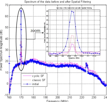
Figure 5 shows the eigenvalues obtained from the clas-sic and the cyclic correlation matrix which were derived from baseband data of the antennas of one station. The cyclic frequency, α, of the pager has been first estimated from the data: α = 0.1221 in normalized frequency. The figure shows that the interferer signal subspace can be fairly well estimated using one dimension in the cyclic decomposition, whereas it needs two dimensions in the classic one. The more dimensions are used to remove the interferer, the more information about the cosmic sources is thrown away as well. We used therefore only the eigen-vector corresponding to the strongest eigenvalue to build the projector for both methods. Figure 6 shows the effect of the projector on the pager. Using the cyclic method, the pager is removed more effectively compared with the classic approach.
5. Conclusions
In this paper, we have described two RFI mitigation ap-proaches based on the cyclostationary properties of the RFI. The first method is a blind cyclostationary detec-tor which has been implemented into a real time receiver. The second one is a cyclic spatial filtering. These methods seem to be an attractive alternative to the classic method based on power statistics. Indeed, as shown with simu-lations and experimental results, it leads to interesting performances for cases where there are relatively strong cosmic sources or for cases where the input signals are un-calibrated. Feliachi (to be published) will describe in her upcoming PhD manuscript other applications of cyclosta-tionarity for phased array radio telescopes.
Fig. 6. Spectrum of one antenna output after applying cyclic and classic spatial filtering (p = 8,N = 65536).
Acknowledgements. The authors would like to thank Pierre Colom, DS4-T3 task leader, Observatoire de Paris, France, Philippe Ravier and Rachid Harba, both from the University of Orl´eans, France, for supplying them with helpful materials and remarks. The authors also want to thank the European Commission Framework Program 6, Project SKADS (contract no 011938), the R´egion Centre, the French research consor-tium GDR-ISIS and the Dutch Helena Kluyver female visitor programme for funding part of this work.
References
Serpedin, E., Panduru, F., Sari, I. & Giannakis, G. B. 2005, Bibliography on cyclostationarity (Signal Processing),12, 85
Weber, R., Viou, C., Coffre, A., Denis, L., et al. 2005,DSP-Enabled Radio Astronomy: Towards IIIZW35 Reconquest (JASP),16
Boonstra, A. J. 2005, Radio Frequency Interference Mitigation in Radio Astronomy, Thesis, Delft university, The Netherlands.
Gardner, W.A, Napolitano, A.& Paura, L. 2006, Cyclostationarity: Half a century of research (Signal Processing), 4 ,86
Weber, R., Zarka, P., Ryabov, V. B., Feliachi, R., et al. 2007, Data preprocessing for decametre wavelength exo-planet detection: an example of cyclostationary rfi detector (Eusipco’2007),Poznan, Poland.
Boonstra, A. J., Weber, R. eds. 2009, RFI Mitigation Methods Inventory, SKADS DS4T3 Report
Feliachi, R., Weber, R., Boonstra, A. J. 2009, Cyclic spatial filtering in radio astronomy : application to LOFAR data (Eusipco’2009), Glasgow, Scotland.
Feliachi, R. to be published, Spatial processing of cyclostation-ary interferers for phased arrays radio telescopes, Thesis, University of Orl´eans, France