HAL Id: hal-02277192
https://hal-univ-rennes1.archives-ouvertes.fr/hal-02277192
Submitted on 8 Jul 2020
HAL is a multi-disciplinary open access
archive for the deposit and dissemination of
sci-entific research documents, whether they are
pub-lished or not. The documents may come from
teaching and research institutions in France or
abroad, or from public or private research centers.
L’archive ouverte pluridisciplinaire HAL, est
destinée au dépôt et à la diffusion de documents
scientifiques de niveau recherche, publiés ou non,
émanant des établissements d’enseignement et de
recherche français ou étrangers, des laboratoires
publics ou privés.
Traboulsi, Fabrice Wendling, Mahmoud Hassan
To cite this version:
Aya Kabbara, Mohamad Khalil, Georges O’Neill, Kathy Dujardin, Youssof El Traboulsi, et al..
Detect-ing modular brain states in rest and task. Network Neuroscience, MIT Press, 2019, 3 (3), pp.878-901.
�10.1162/netn_a_00090�. �hal-02277192�
Detecting modular brain states in rest and task
Aya Kabbara1,2,3, Mohamad Khalil1,3, Georges O’Neill4, Kathy Dujardin5,6,Youssof El Traboulsi7, Fabrice Wendling2, and Mahmoud Hassan2
1Azm Center for Research in Biotechnology and Its Applications, EDST, Lebanese University, Beirut, Lebanon 2University of Rennes, LTSI - U1099, Rennes, France
3CRSI Lab, Engineering Faculty, Lebanese University, Beirut, Lebanon
4Sir Peter Mansfield Imaging Centre, School of Physics and Astronomy, University of Nottingham, University Park, Nottingham, United Kingdom
5INSERM, U1171, Lille, France
6CHU Lille, Neurology and Movement Disorders Department, Lille, France 7LaMA-Liban, Lebanese University, Tripoli, Lebanon
Keywords: Brain network dynamics, Functional connectivity, M/EEG source-space networks
ABSTRACT
The human brain is a dynamic networked system that continually reconfigures its functional connectivity patterns over time. Thus, developing approaches able to adequately detect fast brain dynamics is critical. Of particular interest are the methods that analyze the modular structure of brain networks, that is, the presence of clusters of regions that are densely interconnected. In this paper, we propose a novel framework to identify fast modular states that dynamically fluctuate over time during rest and task. We started by demonstrating the feasibility and relevance of this framework using simulated data. Compared with other methods, our algorithm was able to identify the simulated networks with high temporal and spatial accuracies. We further applied the proposed framework on MEG data recorded during a finger movement task, identifying modular states linking somatosensory and primary motor regions. The algorithm was also performed on dense-EEG data recorded during a picture naming task, revealing the subsecond transition between several modular states that relate to visual processing, semantic processing, and language. Next, we tested our method on a dataset of resting-state dense-EEG signals recorded from 124 patients with Parkinson’s disease. Results disclosed brain modular states that differentiate cognitively intact patients, patients with moderate cognitive deficits, and patients with severe cognitive deficits. Our new approach complements classical methods, offering a new way to track the brain modular states, in healthy subjects and patients, on an adequate task-specific timescale.
AUTHOR SUMMARY
The brain is a dynamic modular network. Thus, exploring the dynamic behavior of the brain can reveal insights about its characteristics during rest and task, in healthy and pathological conditions. In this paper, we propose a new framework that aims to track the dynamic changes of the modular brain organization. The method presents two algorithms that can be applied during task-free or task-related paradigms. Using simulations, we demonstrated the advantages of the proposed algorithm over existing methods. The proposed algorithm was also tested on three datasets recorded from real EEG and MEG acquisitions. Overall, results showed the capacity of the proposed algorithm to track brain network dynamics with good spatial and temporal accuracy.
a n o p e n a c c e s s j o u r n a l
Citation: Kabbara, A., Khalil, M., O’Neill, G.,Dujardin, K., El Traboulsi, Y., Wendling, F. & Hassan, M. (2019). Detecting modular brain states in rest and task.Network Neuroscience, 3(3),
878–901. https://doi.org/10.1162/ netn_a_00090 DOI: https://doi.org/10.1162/netn_a_00090 Supporting Information: https://doi.org/10.1162/netn_a_00090 https://github.com/librteam/ Modularity_algorithm_NN Received: 3 January 2019 Accepted: 18 April 2019
Competing Interests: The authors have declared that no competing interests exist. Corresponding Author: Aya Kabbara [email protected] Handling Editor: Olaf Sporns Copyright:©2019
Massachusetts Institute of Technology Published under a Creative Commons Attribution 4.0 International (CC BY 4.0) license
INTRODUCTION
The human brain is a modular dynamic system. Following fast neuronal activity (Pfurtscheller & Aranibar,1977;Pfurtscheller & Lopes Da Silva,1999), the spatiotemporal organization of rest-ing (Baker et al.,2014;Damaraju et al.,2014;de Pasquale et al.,2012;de Pasquale, Della Penna, Sporns, Romani, & Corbetta,2015;Kabbara, El Falou, Khalil, Wendling, & Hassan,2017) and task-evoked connectivity (Bola & Sabel,2015;Hassan, Benquet, et al.,2015;Hutchison et al.,
2013;O’Neill, Tewarie, Colclough, et al.,2017) is in constant flux.
Hence, an appropriate description of time-varying connectivity is of utmost importance to understand how cognitive and behavioral functions are supported by networks. In this context, several frameworks have been suggested to explore the time-varying nature of func-tional brain connectivity. Among them, hidden Markov model approaches (Baker et al.,2014;
Vidaurre et al.,2017), K-means clustering (Allen, Damaraju, Eichele, Wu, & Calhoun,2017;
Allen et al.,2014;Damaraju et al.,2014), independent component analysis (ICA;O’Neill, Tewarie, Colclough, et al.,2017), principal component analysis (Preti & Van De Ville,2016), or orthogonal connectivity factorization (Hyvärinen, Hirayama, Kiviniemi, & Kawanabe,2016) have been applied to identify the main brain networks shaping dynamic functional connec-tivity. These methods consist of grouping the temporal networks into states, where each state
Dynamic functional connectivity: Measurement of transient changes in the functional brain network across time.
reflects a unique spatial connectivity pattern. It is important to note that in these frameworks, states are identified without looking at the modular organization of the networks.
However, because of the modular organization of the human brain network (Sporns & Betzel,2016) methods for detecting network communities (or modules) are of particular
inter-Module:
A subnetwork composed of strongly connected nodes that are weakly connected to the rest of the network.
est (Sporns & Betzel,2016). These methods decompose the network into building blocks or modules that are internally strongly connected, often corresponding to specialized functions. Importantly, during a learning task, Basset et al. showed that the flexibility (defined as how often a given node changes its modular affiliation over time) of the networks facilitates the prediction of individual future performances in next learning sessions (Bassett et al.,2011), remembering, attention, and integrated reasoning (Gallen et al.,2016).
To compute modularity in networks collected across multiple slices (time points), one could simply decompose each network independently. Another algorithm proposed to link corre-sponding nodes across slices before generating communities. This algorithm is known as multislice modularity (also called multilayer modularity;Mucha, Richardson, Macon, Porter, & Onnela,2010), which has been used to follow changes of the modular architecture in differ-ent applications (Bassett et al.,2011;Bassett, Yang, Wymbs, & Grafton,2015). However, the problem with solely applying these techniques is that they may not lead to easily interpretable results because of the particularly high number of modular structures generated. More
specifi-Modular structure:
The partition of the network into nonoverlapping modules.
cally, the dynamic modular structures obtained are technically difficult to visualize since their number is equal to the number of slices. Alternatively, one could use the multislice modularity algorithm to generate a community structure consistent over time. But such a strategy will con-strain the dynamic analysis. Hence, it would be very useful to find the main modular structures driving the dynamics of neural activity. To date, there is no automatic framework that is able to decipher modular brain states, that is, subsets of brain modules implicated in a given brain
Brain state:
A network pattern representing time points that share some similar topological properties.
function at a given time period.
Here, we propose a novel framework aiming to elucidate the main modular brain struc-tures, called modular states (MS), that fluctuate over time during rest and task. We attempt to find the modular structures that share the same topology by quantifying the similarity be-tween all the computed temporal partitions (Figure 1). The proposed framework simply takes
Figure 1. The algorithm procedure. (A) Computation of modules for each temporal network (Wt).
(B) Assessment of the similarity between the dynamic modular structures. (C) Clustering the similarity matrix into “categorical modules.”
as input a set of connectivity matrices, without making any constraint on how these matrices are computed. This means that it is independent of the choice of the connectivity method, the frequency range of interest, the temporal resolution of dynamic connectivity, and the regions of interest (ROIs). Connectivity matrices could be also extracted from different individuals, or different experimental conditions. The main purpose of the framework is to find the common modular states between the connectivity patterns interpreted. In the paper, we used simulated data to show the advantages of our method over other existing methods in terms of spatial and temporal accuracy. Then, using three different MEG/EEG datasets, recorded in rest and task from healthy subjects and/or patients, we demonstrate the feasibility of the method to reveal both time-varying functional connectivity and the corresponding spatial patterns, as compared
Functional connectivity: Statistical dependency between spatially separated brain regional time series.
with the state-of-the art findings. Overall, findings show that the algorithm was able to track the dynamics of brain networks in adapted timescale, offering a new way to explore the spa-tiotemporal organization of brain function.
MATERIALS AND METHODS
We have developed two versions of the algorithm: (a) “categorical,” where we aim to find the main modular structures over time, with no interest in their sequential order; and (b) “con-secutive,” where the objective is to find the modular structures in a successive way. The two versions are described hereafter.
Categorical Version
The categorical version includes three main steps:
(1) Decompose each temporal network into modules (i.e., clusters of nodes that are inter-nally strongly connected, but exterinter-nally weakly connected;Figure 1A). To do that, different modularity algorithms were proposed in the literature (Blondel, Guillaume, Lambiotte, & Lefebvre,2008;Duch & Arenas,2005;Girvan & Newman,2002;Guimerà & Amaral,
2005).
In our study, we adopted the consensus modularity approach that was previously used in many studies (Bassett et al.,2013;Kabbara et al.,2017): Given an ensemble of partitions acquired from the Newman algorithm (Girvan & Newman,2002) and Louvain algorithm (Blondel et al.,2008) repeated for 200 runs, an association matrix is obtained. This results in an N× N matrix (N is the number of nodes), and an element Ai,j represents the number of times the nodes i and j are assigned to the same module across all runs and algorithms. The association matrix is then compared with a null model association matrix generated from a permutation of the original partitions, and only the significant values are retained (Bassett et al.,2013). To ultimately obtain consensus communities, we reclustered the association matrix using the Louvain algorithm.
(2) Assess the similarity between the temporal modular structures (Figure 1B). In this context, several methods have been suggested to compare community structures (Traud, Kelsic, Mucha, & Porter,2008). Here, we focused on the pair-counting method, which defines a similarity score by counting each pair of nodes drawn from theN nodes of a network according to whether the pair falls in the same or in different groups in each partition (Traud et al.,2008). We considered the z-score of Rand coefficient, bounded between 0 (no similar pair placements) and 1 (identical partitions). This yields aT× T similarity matrix, whereT is the number of time windows.
(3) Cluster the similarity matrix into “categorical” modular states (MS) using the consensus modularity method (Figure 1C). This step combines similar temporal modular structures in the same community. Hence, the association matrix of each “categorical” community is computed using the modular affiliations of its corresponding networks.
Consecutive Version
The difference between the two versions of the algorithm is essentially in the third step, in which the final communities were defined. Particularly, the similarity matrix is segmented in a sequential way using the following steps:
(1) Threshold the similarity matrix using an automatic thresholding algorithm described in Genovese, Lazar, and Nichols (2002). Briefly the matrix was converted into a p value map that is then thresholded based on the false discovery rate (FDR) controlling. (2) Apply a median filter in order to get a smoother presentation of the similarity matrix. (3) Segment the matrix in a sequential way following the algorithm illustrated in the flowchart
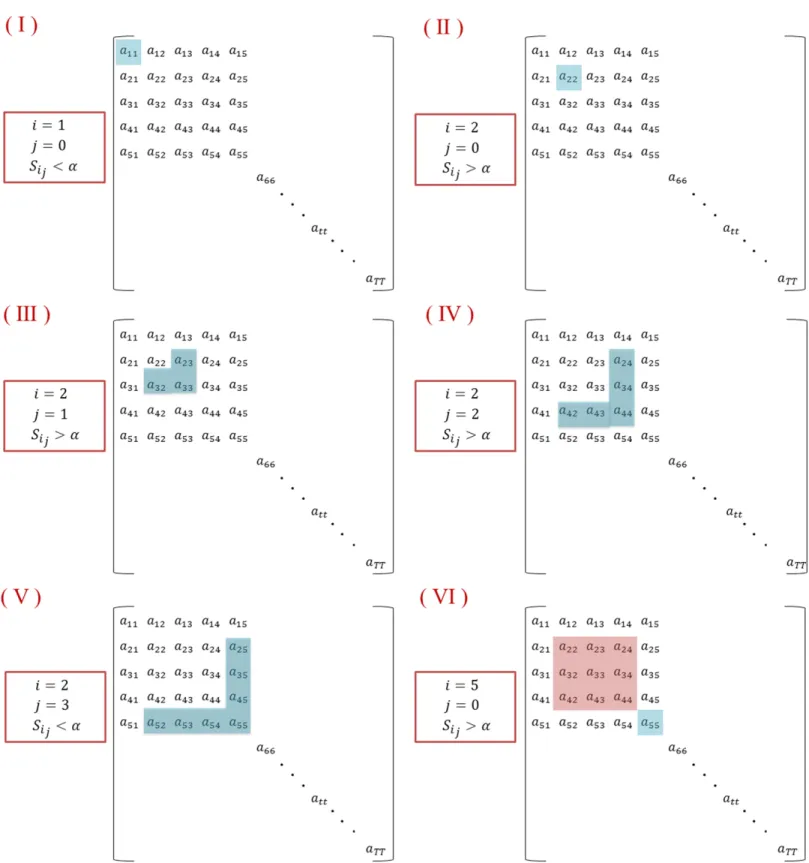
Figure 2. Flowchart of the segmentation algorithm.
modular structures show high similarity values with each other, the algorithm detects the squares located around the diagonal of the similarity matrix. As presented inFigure 2, the condition for which two consecutive structures are associated with the same state is the following:
Si,j > a,
whereSi,j = ∑jk=0ai+j,i+k+ ∑jk=0ai+k,i+j− ai+j,i+j;i, j ∈ [1, T], where al,m denotes the similarity value between the modular structure corresponding to the time windowl and that corresponding to the time windowm.
a is the “accuracy parameter,” strictly bounded between 0 and 1. It regulates the temporal-spatial accuracy of detected modular states. We recommend choosing an adaptive value of a. In this paper, a equals the average of the similarity matrix. A segment is considered to be relevant if the number of included time windows is greater thanjmin(the minimal size allowed for a segment).
The algorithm is illustrated inFigure 3. (I): Starting withi= 1, j = 0; and considering that a11 is lower thana, we obtained S1,0= a11< a, and the algorithm moves to the next time window i= 2. (II): As S2,0= a22is greater thana, j is incremented by 1. (III): Having S2,1= a23+a323+a33> a, the second and the third time windows are associated with the segment. (IV): The algorithm succeeds to add also the fourth time window asS2,2 = a24+a42+a34+a43+a44
5 > a. (V): Then, for
j= 3, we obtain S2,3 = a25+a35+a45+a755+a52+a53+a54 < a. This means that the fifth time window differs from the previous windows in its modular structure. Afterwards, the algorithm moves toward finding another segment by incrementingi and repeating the process (IV).
For each detected segment, the modular structure is obtained after computing the associa-tion matrix of the corresponding time windows modular affiliaassocia-tions.
The Matlab code developed to apply the algorithm in the two versions is publicly available (Kabbara et al.,2019).
Simulated Data
We simulated the adjacency tensor data following the methodology applied inO’Neill, Tewarie, Colclough, et al.(2017). Briefly, fourN× N adjacency matrices Pjwere constructed, where j ∈ [1, 4] and N is the number of ROIs. We used an anatomical atlas of 221 ROIs with the mean of the Desikan-Killiany atlas (Desikan et al.,2006) subdivided byHagmann et al.(2008), yielding to N = 221. The adjacency matrices and the 3-D visualization of the networks are presented inFigure 4A. Following this step, the time evolution of dynamic connectivity in each network is given by the following:
Mj(t) = a. f1j(t) + b. f2j(t);
f1j(t) is the modulation function, which was represented by the Hanning window of unit amplitude;f2j(t) represents uncorrelated Gaussian noise added to the simulated time courses; anda and b are scalar values set to 0.45 and 0.15 as inO’Neill, Tewarie, Colclough, et al.
(2017).
In our study, Mj(t) is sampled at 3.3 Hz (to obtain a sliding window of 0.3 s as in real
data). The onset as well as the duration of each module structure is illustrated inFigure 4B. We then combined the four network matrices in order to generate a single adjacency matrix at each time pointt over a time course spanning 60 s. As a final step, we added a random Gaussian noise to the adjacency tensor, and the standard deviation of the noise was allowed to vary between 0.2 and 0.5.
Validation
On simulated data, we evaluated the performance of the algorithm by computing the simi-larity between the reconstructed and the simulated (reference) networks, taking into account both spatial and temporal similarities. The spatial similarity is given by the z-score of Rand coefficient between the simulated and the constructed modular structures, while the temporal similarity represents the rate of the correct affiliation of time windows.
In addition, we have compared our algorithm with three methods originally developed to identify the brain states without looking at their modular structures. The three methods are K-means clustering as applied byAllen et al.(2014), independent component analysis as suggested byO’Neill, Tewarie, Colclough, et al.(2017), and the consensus clustering algorithm proposed byRasero et al.(2017). For each method, we followed the same pipeline adapted by the authors. To ultimately obtain the modular brain states, we preceded the analysis by decomposing each connectivity state to modules using the consensus modularity approach as detailed in the Categorial Version section.
Real Data
In order to track the brain network dynamics effectively, we particularly tested our method using electro- and magnetoencephalography (EEG/MEG), which allow the tracking of brain dynamics on a subsecond timescale, a resolution not reachable using other techniques such as functional magnetic resonance imaging (fMRI;Cohen,1972;Nunez & Srinivasan,2007;
Figure 4. The simulation scenario. (A) Left: The adjacency matrixPjof the constructed networks. Right: The 3-D cortical presentation of the modular structures of the simulated networks. (B) The time axis showing the beginning and the end of each networkMj(which was generated by combining Pjto uncorrelated noise).
Thus, three M/EEG datasets were analyzed. Before applying the algorithm, we reconstucted the functional brain networks at the level of the cortex using an emerging technique called EEG source connectivity (Chavez et al.,2013;De Vico Fallani et al.,2008;De Vico Fallani, Latora, & Chavez,2017;De Vico Fallani, Richiardi, Chavez, & Achard,2014;Hassan, Shamas, Khalil,
El Falou, & Wendling,2015;Hassan & Wendling,2018;Kabbara et al.,2017;Lai, Demuru, Hillebrand, & Fraschini,2018;Schoffelen & Gross,2009). In order to remove any bias from our analysis, we have generated the dynamic functional connectivity matrices according to how they were computed in the three previous studies that interpreted the data (Hassan, Benquet, et al.,2015;Hassan et al.,2017;O’Neill, Tewarie, Colclough, et al.,2017) The aim of this work is to test whether the modular states generated by our algorithm match the findings obtained in the literature.
Dataset 1: Self-paced motor task for healthy participants (MEG data). Previously used inO’Neill et al.(2015);O’Neill, Tewarie, Colclough, et al.(2017), andVidaurre et al.(2016), this dataset includes 15 participants (9 male, 6 female) asked to press a button using the index finger of their dominant hand, once every 30 s. Using a 275-channel CTF MEG system (MISL; Coquitlam, BC, Canada), MEG data were recorded at a sampling rate of 600 Hz. MEG data were coreg-istered with a template MRI. The cortex was parcellated using the Desikan-Killiany atlas (68 regions;Desikan et al.,2006). The preprocessing, the source reconstruction, and the dynamic functional connectivity computations were performed similarly to those inO’Neill, Tewarie, Colclough, et al. (2017). Briefly, the preprocessing comprises the exclusion of trials (t = −12s → 12s) contaminated by noise. Then, source time courses were reconstructed using a beamforming approach (please refer toO’Neill, Tewarie, Colclough, et al.,2017, for more details). Afterwards, the regional time series were symmetrically orthogonalized following the method proposed inColclough, Brookes, Smith, & Woolrich(2015) to remove the effects of “signal leakage.” The amplitude envelopes of the time courses were obtained using a Hilbert transform. Finally, the dynamic connectivity was estimated by the Pearson correlation measure using a sliding window approach of 6 s of length. The sliding window was shifted by 0.5 s over time. The number of connectivity matrices obtained for each trial was then 49. A statistical threshold (FDR) approach was used to threshold the matrices (Genovese, Lazar, & Nichols,
2002). This yields to a set of connectivity matrices that are thresholded and weighted. Then, the consecutive scheme of the proposed method was tested.
Dataset 2: Picture naming task for healthy participants (dense-EEG data). Twenty-one right-handed healthy subjects (11 women and 10 men) with no neurological disease participated in this study. In a session of about 8 min, each participant was asked to name 148 displayed pictures on a screen using E-Prime 2.0 software (Psychology Software Tools, Pittsburgh, PA;Schneider, Eschman, & Zuccolotto,2002). Oral responses were recorded to set the voice onset time. This study was approved by the National Ethics Committee for the Protection of Persons (CPP), ConneXion study, agreement number 2012-A01227-36, and promoter, Rennes University Hos-pital. All participants provide their written informed consent to participate in this study. A typi-cal trial started with the appearance of an image during 3 s followed by a jittered interstimulus interval of 2 or 3 s randomly. Errors in naming were discarded from the analysis. A total of 2,926 on 3,108 events were considered.
Dense-EEG data were recorded using a system of 256 electrodes (EGI, Electrical Geodesic, Inc.). EEGs were collected at 1 kHz sampling frequency and bandpass filtered between 3 and 45 Hz. The preprocessing and the computation of the functional connectivity followed the same pipeline applied inHassan, Benquet, et al.(2015). In brief, each trial (t= 0 → 600 ms) was visually inspected, and epochs contaminated by eye blinks, muscle movements, or other noise sources were rejected. As described in the previous study (Hassan, Benquet, et al.,2015), the source connectivity method was performed using the wMNE/PLV (phase locking value)
Phase locking value:
A measure used to quantify the statistical coupling, in term of phase
Authors also used the Destrieux atlas subdivided into 959 regions (Hassan, Benquet, et al.,
2015). To remove spurious connections from the dynamic connectivity matrices, we have adopted a statistical threshold based on FDR (Genovese et al.,2002). Finally, a weighted and thresholded connectivity tensor of dimension 959× 959 × 600 was obtained and analyzed using the consecutive scheme of our algorithm.
Dataset 3: Resting state in Parkinson’s disease patients (dense-EEG data). This dataset includes
Resting state:
An experimental paradigm in which the subject is asked to relax and to do nothing.
124 patients with idiopathic Parkinson’s disease defined according to the UK Brain Bank cri-teria for idiopathic Parkinson’s disease (Gibb & Lees, 1988). These patients were separated into three groups: (G1) cognitively intact patients (N= 63); (G2) patients with mild cognitive deficits (N = 46); and (G3) patients with severe cognitive impairment (N = 15). All partic-ipants gave their informed consent to participate in the study, which had been approved by the local institutional review boards (CPP Nord-Ouest IV, 2012-A 01317-36, ClinicalTrials.gov Identifier: NCT01792843). Dense-EEG were recorded with a cap (Waveguard, ANT software BV, Enschede, Netherlands) with 122 scalp electrodes distributed according to the interna-tional system 10-05 (Oostenveld & Praamstra,2001). Electrode impedance was kept below 10 kΩ. Patients were asked to relax without performing any task. Signals were sampled at 512 Hz and bandpass filtered between 0.1 and 45 Hz.
The data were preprocessed according toHassan et al.(2017) dealing with the same dataset. Briefly, EOG artifact detection and correction was applied following the method developed inGratton, Coles, & Donchin(1983). Afterwards, epochs with voltage fluctuation between 90μV and−90 μV were kept. For each participant, two artifact-free epochs of 40-s lengths were selected. This epoch length was used previously and considered as a good compromise between the needed temporal resolution and the reproducibility of the results in resting state (Kabbara et al.,2017).
To compute the dynamic functional connectivity, the steps adopted here are the same used in many previous studies (Hassan et al.,2017;Kabbara et al.,2018,2017). First, EEG data were coregistered with a template MRI through identification of the same anatomical landmarks (left and right preauricular points and nasion). Second, the lead field matrix was computed for a cortical mesh with 15,000 vertices using the OpenMEEG package (Gramfort, Papadopoulo, Olivi, & Clerc, 2010) available in Brainstorm. The noise covariance was estimated using a 1-min resting segment. After that, the time series of EEG sources were estimated using the wMNE algorithm where the regularization parameter was set according to the signal to noise ratio (λ = 0.1 in our analysis). An atlas-based segmentation approach was used to project EEGs onto an anatomical framework consisting of 68 cortical regions identified by means of the Desikan-Killiany atlas (Desikan et al., 2006). The dynamic functional connectivity was then computed using a sliding window over which PLV was calculated (Lachaux, Rodriguez, Martinerie, & Varela,1999). In the previous study (Hassan et al.,2017), the disruptions of the functional connectivity were found in the alpha 2 band (10–13 Hz). For this reason, we con-sidered the same frequency band in our analysis. To obtain a sufficient number of cycles at the given frequency band, we chose the smallest window length that is equal to central frequency6 , as recommended inLachaux et al.(1999). This yields a sliding window of 0.52 s. We then adopted a proportional threshold of 10% to maintain only the top 10% of correlation values of the connectivity matrix. These steps produce, for each epoch, a weighted thresholded con-nectivity tensor of dimensionN× N × T, where N is the number of ROIs (68 regions) and T is the number of time windows (77 time windows). This tensor is formally equivalent to dynamic functional connectivity matrices, and it was analyzed using the categorical version of the proposed algorithm.
RESULTS
Having the set of connectivity matrices, we first applied a community detection algorithm (Louvain method) to decompose each network into modules (i.e., clusters of nodes that are internally strongly connected, but externally weakly connected). The similarity between the temporal modular structures was calculated (Figure 1B). Finally, the modular states (MS) were obtained by applying a community detection algorithm to the similarity matrix (Figure 1C).
We propose two different frameworks: (a) “categorical,” where the objective is to find the main modular structures, without any interest in their sequential order; and (b) “consecutive,” where the objective is to find the modular structures in a successive way.
Validation on Simulated Data
Figure 5shows the results of the categorical method applied on the dynamic networks gen-erated by the simulation scenario (STDnoise= 0.2). Four modular states were obtained: MS1,
MS2, MS3, and MS4.Figure 5Aillustrates the modular states’ time courses, showing the most likely state at each time window, whileFigure 5Bshows the 3-D representation of the MS. Qual-itatively, the four simulated modular structures have been successfully reconstructed. However, one time window that actually belongs to the background (i.e., random) has been wrongly affiliated with MS2. Moreover, the MS3 state time course presented two false time window detections: one belongs to MS4, and the other belongs to the background. To quantitatively validate the obtained results, we compared the simulated structures (M1, M2, M3, and M4) with the reconstructed structures (MS1, MS2, MS3, and MS4) in terms of spatial and temporal
Figure 5. Results of the categorical method applied on simulated data. (A) The time course of the
four modular structures reconstructed. The gray square indicates false time window detection. (B) The 3-D representation of the four modular structures’ states.
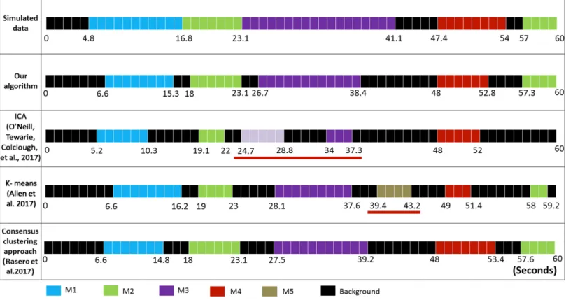
Figure 6. Results of the consecutive method applied on simulated data. (A) The results of the
segmentation algorithm used to derive the consecutive modular structures from the similarity matrix by (1) thresholding the matrix using FDR, (2) applying a median filter on the thresholded matrix, and (3) extracting the most significant segments. (See the Methods section for more details about the consecutive algorithm steps.) (B) The 3-D representation of the five consecutive modular structures obtained. (C) The difference between the simulated time axis and the obtained time axis.
similarities. The spatial similarities between the simulated and the reconstructed data are 0.99, 0.98, 0.99, and 0.98 for MS1, MS2, MS3, and MS4, respectively. The temporal similarities are 0.79, 0.83, 0.9, and 0.71 for MS1, MS2, MS3, and MS4, respectively. On average, the cate-gorical method achieved spatial accuracy of 98.5% and a temporal accuracy of 80.8%.
Using the consecutive method, the algorithm has segmented the similarity matrix yielding to the detection of five modular states (Figure 6A). Their 3-D representations are shown in
Figure 6B. One can remark that MS1 (spatial similarity= 0.94; temporal similarity = 0.88), MS2 (spatial similarity= 0.99; temporal similarity = 0.94), MS3 (spatial similarity = 0.97; temporal similarity= 0.77), MS4 (spatial similarity = 1; temporal similarity = 0.88), and MS5 (spatial similarity= 0.95; temporal similarity = 1) matched, temporally and spatially, the simulated networks generated at the corresponding time windows. In addition, one can remark that the algorithm hasn’t produced false positive results. Globally, the assessed spatial and temporal accuracies are 94% and 83%, respectively.
Results corresponding toSTDnoise= 0.35; STDnoise= 0.5 are illustrated in theSupporting Information. In brief, results show that using the categorical algorithm, the spatial characteriza-tions of the four modular states were successfully detected. However, the state time course of MS3 failed to detect the second corresponding segment (Figures 1and2in the Supporting In-formation). Using the consecutive algorithm, the five MSs were temporally detected (Figures 3
and4in the Supporting Information).
The difference between the simulated time axis and the obtained time axis using other differ-ent algorithms is presdiffer-ented inFigure 7. Using ICA (O’Neill, Tewarie, Colclough, et al.,2017), five independent components (ICs) were detected: IC1, IC2, and IC5 correspond, respectively,
Table 1. Temporal similarities between the simulated MSs and those obtained using the different algorithms
Algorithm MS1 MS2 MS3 MS4 MS5 False positive rate Average temporal similarity
Our algorithm 0.73 0.98 0.67 0.86 0.93 0 0.83
ICA (O’Neill, Tewarie, Colclough, et al., 2017)
0.43 0.6 0.41 0.71 0 0 0.43
K-means
(Allen et al.,2017)
0.8 0.77 0.53 0.61 0.55 0.07 0.58
Consensus clustering approach (Rasero et al.,2017)
0.68 0.98 0.65 0.79 0.85 0 0.79
to M1 (spatial similarity= 0.96; temporal similarity = 0.43), M2 (spatial similarity = 0.85; temporal similarity= 0.60), and M4 (spatial similarity = 0.86; temporal similarity = 0.71). However, M3 (spatial similarity= 0.94; temporal similarity = 0.42) was reflected by two sep-arated components: IC3 and IC4. One can realize also that the ICA algorithm failed to detect M2 spanning between 57 ms and 60 ms. Using K-means clustering (Allen et al.,2014), six brain states (BSs) were generated. BS1, BS2, BS3, BS5, and BS6 correspond, respectively, to M1 (spatial similarity= 0.96; temporal similarity = 0.8), M2 (spatial similarity = 0.94; tem-poral similarity= 0.77), M3 (spatial similarity = 0.97; temporal similarity = 0.53), M4 (spatial similarity= 1; temporal similarity = 0.61), and M5 (spatial similarity = 0.99; temporal similar-ity = 0.55). While the five simulated modular states were reconstructed, a false time win-dow detection was captured (BS4). Regarding the consensus clustering algorithm proposed by
Rasero et al.(2017), the algorithm succeeded to detect the five simulated states.Tables 1and2
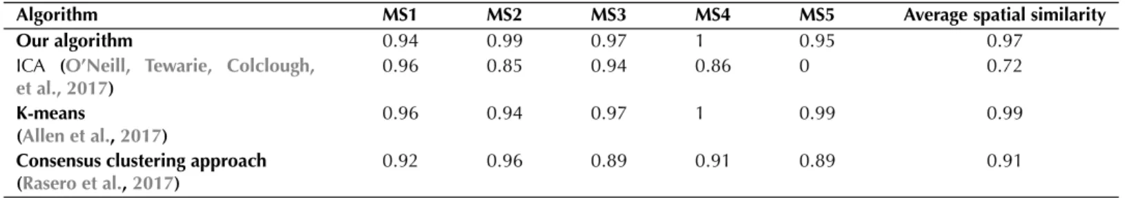
report the temporal and spatial similarities between the simulated MSs and those obtained us-ing the different algorithms. Overall, results show that our algorithm reached the highest tem-poral detection accuracy (0.83) compared with ICA (0.43), K-means clustering (0.58), and the consensus clustering (0.79). Spatially, our algorithm procured a good spatial similarity (0.97), outperforming ICA (0.72) and the consensus clustering algorithms (0.91).
Real Data
Dataset 1: Self-paced motor task for healthy participants (MEG data). As the considered dataset is collected during a task-related paradigm, our objective was to follow the spatiotemporal
Task-related paradigm:
An experimental paradigm in which the subject is asked to focus on a specific function.
organization of the dynamic brain networks during time (from the stimulus onset to the reaction time). Thus, we applied the consecutive algorithm to track the MSs in a successive way. The input of the algorithm is the tensor of dynamic connectivity matrices averaged over all trials and subjects. The same dataset and methods were previously used inO’Neill et al.(2015),
O’Neill, Tewarie, Colclough, et al.(2017), andVidaurre et al.(2016). The algorithm results in
Table 2. Spatial similarities between the simulated MSs and those obtained using the different algorithms
Algorithm MS1 MS2 MS3 MS4 MS5 Average spatial similarity
Our algorithm 0.94 0.99 0.97 1 0.95 0.97
ICA (O’Neill, Tewarie, Colclough, et al., 2017)
0.96 0.85 0.94 0.86 0 0.72
K-means
(Allen et al.,2017)
0.96 0.94 0.97 1 0.99 0.99
Consensus clustering approach (Rasero et al.,2017)
Figure 8. The MS of the MEG motor task obtained using the consecutive method.
one significant MS found between−0.5 s and 1.5 s (Figure 8). As illustrated, this module impli-cates the sensory motor area, the post- and precentral regions of both hemispheres.
Dataset 2: Picture naming task for healthy participants (dense-EEG data). The objective of using this dataset was to track the fast space/time dynamics of functional brain networks at subsecond timescale from the onset (presentation of the visual stimuli) to the reaction time (articulation). Hence, the consecutive version was applied on the dynamic connectivity matrices averaged over subjects.
Figure 9shows the results, revealing that the cognitive process can be divided into five modular structures: The first MS corresponds to the time period ranging from the stimulus onset
Figure 9. The sequential MSs of the EEG picture naming task obtained using the consecutive
to 130 ms and presents one module located mainly in the occipital region. The second MS is observed between 131 and 187 ms, and involves one module showing occipitotemporal connections. The third MS is identified between 188 and 360 ms, and illustrates a module located in the occipitotemporal region, and another module located in the frontocentral region. This structure was then followed by a fourth MS, found over the period 361–470 ms. MS4 was very similar to the previous MS but with additional frontocentral connections. The last MS is observed between 471 and 500 ms, and it shows a module connecting the frontal, central, and temporal regions. It is worth noting that these MSs denote the transitions from the visual processing and recognition to the semantic processing and categorization to the preparation of the articulation process (Hassan, Benquet, et al.,2015;VanRullen & Thorpe,2001).
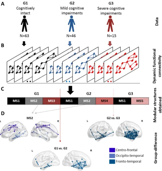
Figure 10. The analysis pipeline and the results of the categorical method applied on the Parkinson’s
disease EEG dataset. (A) The dataset composed of 124 patients partitioned into three groups: (G1) cognitively intact patients (N=63), (G2) patients with mild cognitive deficits (N=46), and (G3) pa-tients with severe cognitive impairment (N=15). (B) The functional dynamic connectivity matrices of the three groups concatenated over time. (C) The five modular structures obtained after applying the categorical algorithm on the concatenated tensor. (D) The modular differences between G1 and G2, G1 and G3, and G2 and G3.
Dataset 3: Resting state in Parkinson’s disease patients (dense-EEG data). Our objective here was to identify the modular structures that are common between G1, G2, and G4, and those that are specific to each group. As the sequential order of MSs is not intended, we applied the cat-egorical version of the proposed algorithm. The latter takes as input the concatenation of the dynamic connectivity matrices of the three groups. This will form a single data tensor of dimen-sionN× N × T, where N is the number of ROIs and T is equal to the number of time windows × the number of patients (Figure 10). The algorithm was then applied to validate the usefulness of the categorical version in detecting the modular alterations between G1, G2, and G3.
Results are illustrated inFigure 10. Five modular structures were identified (MS1, MS2, MS3, MS4, and MS5). Three MSs were found for G1 and G2. However, the number of MSs decreased from three to two MSs in G3. Results revealed that MS1 was found to be present in the three groups, while MS2 was present only in G1 and G2. The modular structure MS2 (absent in G3) is illustrated inFigure 10 and includes two modules involving mainly frontocentral and occipitotemporal connections. The difference between G1 and G2 was reflected by the absence of the structure MS3 replaced by the structure MS4 in G2. Results inFigure 10show that the difference concerns mainly the frontotemporal connections. The difference between G2 and G3 was reflected by the absence of the structure MS4 from G2 and the presence of the structure MS5 in G3.Figure 10shows that the functional disruptions between G2 and G3 are mainly frontotemporal connections. It is worth noting that the frontotemporal disruptions were widely reported in mild cognitive impairments (Beyer, Janvin, Larsen, & Aarsland,2007;
de Haan et al., 2012;Song et al., 2011; Zhang et al., 2009), while the central disruptions are widely observed in severe cognitive impairments (Hassan et al.,2017) and dementia (Song et al.,2011).
DISCUSSION
In this paper, we have developed a novel framework to explore the fast reconfiguration of the functional brain networks during rest and task. This new method can be used to track the sequential evolution of brain modules during a task-directed paradigm or to identify the modular brain states that arise at rest. The simulation-based analysis showed the ability of the method to “reestimate” the modular network structures over time. Compared with other methods, our proposed algorithm reached the highest temporal accuracy detection and a very good spatial accuracy.
The new framework was validated on three different EEG/MEG datasets: (a) MEG data recorded from 15 healthy subjects during a self-paced motor task, (b) dense-EEG data recorded from 21 healthy subjects during a picture naming task, and (c) dense-EEG data recorded at rest from 124 Parkinson’s disease patients with different cognitive phenotypes. Results show that our method can track the fast modular states of the human brain network at a subsecond timescale, and also highlight its potential clinical applications, such as the detection of the cognitive decline in Parkinson’s disease.
“Categorical” and “Consecutive” Processing Schemes
The two processing schemes proposed here are both derived from the similarity matrix between the temporal modules (Steps 1 to 3 in the Methods section). However, each version highlights a specific characterization of the modular structures, which can then be exploited depend-ing on the application (time/condition dependent). In particular, the results of the categorical algorithm on the simulated data reveal high spatial resolution and relatively low temporal resolution compared with those obtained using the consecutive algorithm. The low temporal
resolution of the categorical version is reflected by the false (Figure 5) as well as the missed time windows detection (Figures 1andFigure 2in theSupporting Information). In contrast, these time windows were correctly detected by the consecutive version despite their short length (Figure 6, andSupporting InformationFigures 3 and 4). Yet, the low spatial resolution of the consecutive version can be illustrated by MS5 (Figure 6, andSupporting Information
Figures 3 and 4) that should represent M2 (Figure 4). This is probably due to the categorical version using the maximum number of available data points to generate their corresponding MS, while the consecutive version treats each temporal segment solely.
We suggest using the consecutive version where sequential order of MSs is interesting to in-vestigate, such as the tracking of cognitive tasks. When the temporal aspects are not necessary, we would recommend the categorical version.
Tracking of Fast Cognitive Functions
The brain dynamically reconfigures its functional network structure on subsecond temporal scales to guarantee efficient cognitive and behavioral functions (O’Neill, Tewarie, Vidaurre, et al.,
2017). Tracking the spatiotemporal dynamics of large-scale networks over this short time dura-tion is a challenging issue (Allen et al.,2014;Hutchison et al.,2013). In this paper, we aimed to examine how fast changes in the modular architecture shape information processing and distribution in (a) motor tasks and (b) picture naming tasks.
Concerning the self-paced motor task, it is a simple task where only motor areas are ex-pected to be involved over time. Our results indeed showed that the motor module is clearly elucidated related to the tactile movement of the button press. The spatial and temporal fea-tures of the obtained module are very close to the significant component obtained byO’Neill, Tewarie, Colclough, et al.(2017) using the temporal ICA method.
The different MSs obtained in the EEG picture naming task are temporally and spatially anal-ogous to the network brain states detected using other approaches such as K-means clustering byHassan, Benquet, et al.(2015). In particular, the first MS representing the visual network is probably modulated by the visual processing and recognition processes (Thorpe, Fize, & Marlot,1996; VanRullen & Thorpe, 2001). The second MS reflects the memory access re-flected by the presence of the occipital-temporal connections (Martin & Chao,2001). In other words, the brain tries to retrieve the information related to the picture illustrated from memory (Martin & Chao,2001). In the third and the fourth MSs, we notice the implication of a sep-arated frontal module. This module may be related to the object category recognition (tools vs. animals) and the decision-making process (Andersen & Cui,2009;Clark & Manes,2004;
Rushworth, Noonan, Boorman, Walton, & Behrens,2011). After making the decision, speech articulation and the naming process is prepared and started (Dronkers,1996). This is reflected by the MS5 that combines the frontal, the motor, and the temporal brain areas.
Modular Brain States and Cognitive Phenotypes in Parkinson’s Disease
Emerging evidence shows that Parkinson’s disease (PD) is associated with alteration in struc-tural and functional brain networks (Fornito, Zalesky, & Breakspear, 2015). Hence, from a clinical perspective, the demand is high for a network-based technique to identify the patho-logical networks and to detect early cognitive decline in PD. Here, we used a dataset with a large number (N = 124) of PD patients categorized into three groups in terms of their cogni-tive performance: G1, cognicogni-tively intact patients; G2, patients with mild to moderate cognicogni-tive
deficits; and G3, patients with severe cognitive deficits in all cognitive domains. SeeDujardin et al.(2015),Hassan et al.(2017), andLopes et al. (2017) for more information about this database.
The obtained MSs presented inFigure 10show that while some MSs remain unchangeable during cognitive decline from G1 to G3, others are altered and replaced by new MSs. More specifically, the number of MSs detected in G3 has decreased compared with G1 and G2; MS3 in G1 was replaced by MS4 in G2, while MS4 in G2 was replaced by MS5 in G3. In addition, the alterations in G3 involve more distributed modules (central, frontotemporal) than the alterations occurring between G1 and G2 (frontotemporal modules) where the impairment still moderate.
Interestingly, the underlying modular differences between the MSs of groups are con-sistent with the previously reported studies that explored the network changes in PD (Beyer et al., 2007;Bosboom, Stoffers, Wolters, Stam, & Berendse, 2009;de Haan & Pijnenburg,
2009;Hassan et al.,2017;Song et al.,2011;Zhang et al.,2009). Particularly, the loss of fron-totemporal connections in PD is supported by several EEG and MEG studies (Bosboom et al.,
2009;Hassan et al.,2017;Zhang et al.,2009). Similarly, results of structural MRI studies reveal frontal and temporal atrophies in PD with mild cognitive impairment (Beyer et al.,2007;Song et al.,2011). Other functional (de Haan et al.,2012) and structural (Zhang et al.,2009) studies showed that Alzheimer’s disease networks are characterized by frontotemporal alterations. In addition, the brain regions involved in the modular alterations in G3 found in our study are in line with findings obtained by EEG edgewise analysis (Hassan et al.,2017), and by structural MRI studies showing widespread atrophy associated with PD patients’ related dementia (Song et al.,2011).
Methodological Considerations
First, we used a template anatomical image generated from MRIs of healthy controls for EEG/ MEG source functional connectivity analysis. The template-based method is common practice
EEG/MEG source connectivity: A method used to estimate functional brain networks at the cortical level using EEG/MEG sensors.
in the absence of individual anatomical images and was previously employed by multiple EEG and MEG source reconstruction studies, because of nonavailability of native MRIs (Hassan et al.,2017;Kabbara et al.,2018;Lopez et al.,2014). Furthermore, a recent study showed that there are few potential biases introduced during the use of a template MRI compared with individual MRI coregistration.
Second, the connectivity matrices in Dataset 3 (Parkinson’s disease analysis) were thresh-olded by keeping the highest 10% of the edge’s weights. According to previous studies, the 10% threshold provides an optimal trade-off between retaining the true connections and reduc-ing spurious connections (Lord, Horn, Breakspear, & Walter,2012). However, the consistency of results across a range of proportional thresholds would be interesting to consider. In con-trast, a statistical threshold (FDR) approach was used in Dataset 1 (self-paced motor tasks) and Dataset 2 (picture naming); see Methods. The reason is that in Dataset 3, three groups were compared. The proportional threshold approach, compared with other threshold approaches, ensures equal density between the analyzed groups (van den Heuvel et al., 2017). More-over, studies suggest that FDR controlling procedures are effective for the analysis of neuro-imaging data in the absence of intergroup comparison (Bassett et al.,2013;Genovese et al.,
2002;Patel & Bullmore,2016). One should also note that other strategies and criteria could be used to objectively threshold the connectivity matrices, such as the minimum spanning tree metric (Tewarie, van Dellen, Hillebrand, & Stam,2015) and the efficiency cost optimization (De Vico Fallani et al.,2017).
Third, according to the consecutive algorithm, it is noteworthy that two parameters should be adequately tuned to obtain relevant results: (a) the accuracy parametera, and (b) the min-imal length allowed for a statejmin. In particular, the accuracy parametera will dramatically affect the number and the temporal accuracy of detected states. Thus, it should be appropriately selected. A high value may eliminate strong and significant similarity values in a low-average matrix, whereas a low value may overemphasize weak similarity values in high-average con-nectivity networks. Thus, we recommend choosing an adaptive value determined based on the distribution of the similarity matrix. For this reason, the use of the average value is proposed. In order to evidence our choice, we illustrate, based on simulated data with different noise levels, the number of detected MSs as well the temporal accuracy as a function ofa (Figures 5, 6, and 7 in theSupporting Information). In all cases, results show that the average value of the similarity matrix provides the exact number of MSs and a good temporal accuracy. Concerning the second parameter,jmin, it will depend on the way in which the connectivity matrices are computed. In the case where the connectivity is calculated over a time window that guarantees a sufficient number of data points, there is no need to set a minimal length for a state (jmin= 1). In contrast, when a connectivity matrix is computed at each millisecond, one may restrict the length of a state to be less than a specific number of milliseconds. As an example,Mheich, Hassan, Khalil, Berrou, & Wendling(2015) suggested to reject a brain state that has a time interval less than 30 ms. In our study,jminwas set to 1 time window in simulated data, Dataset 1 and Dataset 3, since an optimal sliding window was used. In Dataset 2, where a connectivity matrix based on the PLV metric was computed each millisecond,jminwas set equal to 30 ms, as proposed byMheich et al.(2015).
Fourth, we are aware that spurious correlations caused by the problem of “source leakage” should be carefully considered. Here, we have adopted in each dataset the same pipeline (from data processing to network construction) used by the previous studies dealing with the same dataset. Thus, for the MEG dataset, the correction for source leakage was performed by the symmetric orthogonalization method proposed byColclough et al.(2015). Using the same pipeline also helps to avoid influencing factors caused by changing the source connectivity method, the number of ROIs, the connectivity measure, or the sliding window length. By rely-ing on previous studies (Hassan, Benquet, et al.,2015;Hassan et al.,2017;O’Neill, Tewarie, Colclough, et al.,2017), we provide appropriate input—already tested and validated—to the algorithm, regardless of how it was obtained. The source leakage issue was extensively dis-cussed in a very recent review about M/EEG source-space networks (Hassan & Wendling,
2018).
In addition, a quantitative comparison presented in the paper was performed between our algorithm, K-means clustering as proposed byAllen et al. (2014), independent component analysis as proposed byO’Neill, Tewarie, Vidaurre, et al.(2017), and the consensus cluster-ing algorithm as proposed byRasero et al.(2017). Nevertheless, other strategies that showed accurate results in previous studies could be also investigated and compared, such as the use of a hidden Markov model (HMM), which models the cortical time series using a probabilis-tic generative model (Vidaurre et al.,2017), or the use of a multivariate autoregressive model (De Vico Fallani et al.,2008).
ACKNOWLEDGMENTS
This work has received a French government support granted to the CominLabs excellence laboratory and managed by the National Research Agency in the “Investing for the Future” program under reference ANR-10-LABX-07-01. It was also financed by the Rennes University
Hospital (COREC Project named conneXion, 2012-14). This work was financed by the Azm Center for Research in Biotechnology and Its Applications. GCO is funded by a Medical Research Council New Investigator Research Grant (MR/M006301/1). This study was also sup-ported by the Future Emerging Technologies (H2020-FETOPEN-2014-2015-RIA under agree-ment No. 686764) as part of the European Union’s Horizon 2020 research and training program 2014–18. The study was also funded by the National Council for Scientific Research (CNRS) in Lebanon.
AUTHOR CONTRIBUTIONS
Aya Kabbara: Conceptualization; Formal analysis; Methodology; Software; Validation; Visu-alization; Writing - Original Draft. Mohamad Khalil: Funding acquisition. Georges O’Neill: Data curation. Kathy Dujardin: Data curation. Youssof El Traboulsi: Methodology. Fabrice Wendling: Funding acquisition. Mahmoud Hassan: Conceptualization; Formal analysis; Super-vision; Writing - Original Draft.
FUNDING INFORMATION
Fabrice Wendling, Rennes University Hospital (http://dx.doi.org/10.13039/501100001665), Award ID: ANR-10-LABX-07-01. Mohamad Khalil, National Council for Scientific Research. Georges O’Neill, Medical Research Council, Award ID: MR/M006301/1. Fabrice Wendling, Hôpital de rennes1, Award ID: COREC Project named conneXion, 2012–14.
REFERENCES
Allen, E. A., Damaraju, E., Eichele, T., Wu, L., & Calhoun, V. D. (2017). EEG signatures of dynamic functional network connec-tivity states. Brain Topography, 1–16. https://doi.org/10.1007/ s10548-017-0546-2
Allen, E. A., Damaraju, E., Plis, S. M., Erhardt, E. B., Eichele, T., & Calhoun, V. D. (2014). Tracking whole-brain connectivity dy-namics in the resting state. Cerebral Cortex, 24, 663–676.https:// doi.org/10.1093/cercor/bhs352
Andersen, R. A., & Cui, H. (2009). Intention, action planning, and decision making in parietal-frontal circuits. Neuron.https://doi. org/10.1016/j.neuron.2009.08.028
Baker, A. P., Brookes, M. J., Rezek, I. A., Smith, S. M., Behrens, T., Smith, P. J. P., & Woolrich, M. (2014). Fast transient networks in spontaneous human brain activity. eLife.https://doi.org/10.7554/ eLife.01867
Bassett, D. S., Porter, M. A., Wymbs, N. F., Grafton, S. T., Carlson, J. M., & Mucha, P. J. (2013). Robust detection of dynamic com-munity structure in networks. Chaos, 23.https://doi.org/10.1063/ 1.4790830
Bassett, D. S., Wymbs, N. F., Porter, M. A., Mucha, P. J., Carlson, J. M., & Grafton, S. T. (2011). Dynamic reconfiguration of hu-man brain networks during learning. Proceedings of the National Academy of Sciences, 108, 7641–7646.https://doi.org/10.1073/ pnas.1018985108
Bassett, D. S., Yang, M., Wymbs, N. F., & Grafton, S. T. (2015). Learning-induced autonomy of sensorimotor systems. Nature Neuroscience, 18, 744–751.https://doi.org/10.1038/nn.3993
Beyer, M. K., Janvin, C. C., Larsen, J. P., & Aarsland, D. (2007). A magnetic resonance imaging study of patients with parkin-son’s disease with mild cognitive impairment and dementia
using voxel-based morphometry. Journal of Neurology, Neuro-surgery, and Psychiatry, 78, 254–259.https://doi.org/jnnp.2006. 093849[pii]\r10.1136/jnnp.2006.093849
Blondel, V. D., Guillaume, J.-L., Lambiotte, R., & Lefebvre, E. (2008). Fast unfolding of communities in large networks. Jour-nal of Statistical Mechanics: Theory and Experiment, 10008, 6.
https://doi.org/10.1088/1742-5468/2008/10/P10008
Bola, M., & Sabel, B. A. (2015). Dynamic reorganization of brain func-tional networks during cognition. NeuroImage, 114, 398–413.
https://doi.org/10.1016/j.neuroimage.2015.03.057
Bosboom, J. L. W., Stoffers, D., Wolters, E. C., Stam, C. J., & Berendse, H. W. (2009). MEG resting state functional con-nectivity in Parkinson’s disease related dementia. Journal of Neural Transmission,116,193–202. https://doi.org/10.1007/s00702-008-0132-6
Chavez, M., De Vico Fallani, F., Valencia, M., Artieda, J., Mattia, D., Latora, V., & Babiloni, F. (2013). Node accessibility in cor-tical networks during motor tasks. Neuroinformatics.https://doi. org/10.1007/s12021-013-9185-2
Clark, L., & Manes, F. (2004). Social and emotional decision-making following frontal lobe injury. Neurocase, 10, 398–403.https:// doi.org/10.1080/13554790490882799
Cohen, D. (1972). Magnetoencephalography: Detection of the brain’s electrical activity with a superconducting magnetome-ter. Science, 175, 664–666.https://doi.org/10.1126/science.175. 4022.664
Colclough, G. L., Brookes, M. J., Smith, S. M., & Woolrich, M. W. (2015). A symmetric multivariate leakage correction for MEG connectomes. NeuroImage, 117, 439–448. https://doi.org/10. 1016/j.neuroimage.2015.03.071
Damaraju, E., Allen, E. A., Belger, A., Ford, J. M., McEwen, S., Mathalon, D. H., . . . Calhoun, V. D. (2014). Dynamic functional connectivity analysis reveals transient states of dysconnectivity in schizophrenia. NeuroImage: Clinical, 5, 298–308.https://doi. org/10.1016/j.nicl.2014.07.003
de Haan, W., & Pijnenburg, Y. (2009). Functional neural network analysis in frontotemporal dementia and Alzheimer’s disease us-ing EEG and graph theory. BMC Neuroscience, 10, 101.https:// doi.org/10.1186/1471-2202-10-101
de Haan, W., Van der Flier, W. M., Koene, T., Smits, L. L., Scheltens, P., & Stam, C. J. (2012). Disrupted modular brain dynamics reflect cognitive dysfunction in Alzheimer’s disease. NeuroImage, 59, 3085–3093.https://doi.org/10.1016/j.neuroimage.2011.11.055
de Pasquale, F., Della Penna, S., Snyder, A. Z., Marzetti, L., Pizzella, V., Romani, G. L., & Corbetta, M. (2012). A cortical core for dy-namic integration of functional networks in the resting human brain. Neuron, 74, 753–764.https://doi.org/10.1016/j.neuron. 2012.03.031
de Pasquale, F., Della Penna, S., Sporns, O., Romani, G. L., & Corbetta, M. (2015). A dynamic core network and global ef-ficiency in the resting human brain. Cerebral Cortex, bhv185.
https://doi.org/10.1093/cercor/bhv185
De Vico Fallani, F., Latora, V., Astolfi, L., Cincotti, F., Mattia, D., Marciani, M. G., . . . Babiloni, F. (2008). Persistent patterns of in-terconnection in time-varying cortical networks estimated from high-resolution EEG recordings in humans during a simple motor act. Journal of Physics A: Mathematical and Theoretical.https:// doi.org/10.1088/1751-8113/41/22/224014
De Vico Fallani, F., Latora, V., & Chavez, M. (2017). A topo-logical criterion for filtering information in complex brain networks. PLoS Computational Biology.https://doi.org/10.1371/ journal.pcbi.1005305
De Vico Fallani, F., Richiardi, J., Chavez, M., & Achard, S. (2014). Graph analysis of functional brain networks: Practical issues in translational neuroscience. Philosophical Transactions of the Royal Society B: Biological Sciences. https://doi.org/10.1098/ rstb.2013.0521
Desikan, R. S., Sugonne, F., Fischl, B., Quinn, B. T., Dickerson, B. C., Blacker, D., . . . Killiany, R. J. (2006). An automated labeling system for subdividing the human cerebral cortex on MRI scans into gyral based regions of interest. NeuroImage, 31, 968–980.
https://doi.org/10.1016/j.neuroimage.2006.01.021
Dronkers, N. F. (1996). A new brain region for coordinating speech articulation. Nature, 384, 159–161.https://doi.org/10. 1038/384159a0
Duch, J., & Arenas, A. (2005). Community detection in complex networks using extremal optimization. Physical Review E, 72, 027104.https://doi.org/10.1103/PhysRevE.72.027104
Dujardin, K., Moonen, A. J. H., Behal, H., Defebvre, L., Duhamel, A., Duits, A. A., . . . Leentjens, A. F. G. (2015). Cognitive disor-ders in Parkinson’s disease: Confirmation of a spectrum of sever-ity. Parkinsonism and Related Disorders, 21, 1299–1305.https:// doi.org/10.1016/j.parkreldis.2015.08.032
Fornito, A., Zalesky, A., & Breakspear, M. (2015). The connectomics of brain disorders. Nature Reviews Neuroscience.https://doi.org/ 10.1038/nrn3901
Gallen, C. L., Baniqued, P. L., Chapman, S. B., Aslan, S., Keebler, M., Didehbani, N., & D’Esposito, M. (2016). Modu-lar brain network organization predicts response to cognitive training in older adults. PLoS ONE, 11.https://doi.org/10.1371/ journal.pone.0169015
Genovese, C. R., Lazar, N. A., & Nichols, T. (2002). Thresholding of statistical maps in functional neuroimaging using the false dis-covery rate. NeuroImage, 15, 870–878.https://doi.org/10.1006/ nimg.2001.1037\rS1053811901910377[pii]
Gibb, W. R. G., & Lees, A. J. (1988). The relevance of the Lewy body to the pathogenesis of idiopathic Parkinson’s disease. Jour-nal of Neurology, Neurosurgery, and Psychiatry.https://doi.org/ 10.1136/jnnp.51.6.745
Girvan, M., & Newman, M. E. J. (2002). Community structure in social and biological networks. Proceedings of the National Academy of Sciences, 99, 7821–7826.https://doi.org/10.1073/ pnas.122653799
Gramfort, A., Papadopoulo, T., Olivi, E., & Clerc, M. (2010). Open-MEEG: Opensource software for quasistatic bioelectromagnetics. Biomedical Engineering Online, 9, 45.https://doi.org/10.1186/ 1475-925X-9-45
Gratton, G., Coles, M. G. H., & Donchin, E. (1983). A new method for off-line removal of ocular artifact. Electroencephalography and Clinical Neurophysiology, 55, 468–484.https://doi.org/10. 1016/0013-4694(83)90135-9
Guimerà, R., & Amaral, L. A. N. (2005). Functional cartography of complex metabolic networks. Nature, 433, 895–900.https://doi. org/10.1038/nature03288
Hagmann, P., Cammoun, L., Gigandet, X., Meuli, R., Honey, C. J., Van Wedeen, J., & Sporns, O. (2008). Mapping the structural core of human cerebral cortex. PLoS Biology, 6, 1479–1493.https:// doi.org/10.1371/journal.pbio.0060159
Hassan, M., Benquet, P., Biraben, A., Berrou, C., Dufor, O., & Wendling, F. (2015). Dynamic reorganization of functional brain networks during picture naming. Cortex, 73, 276–288.https:// doi.org/10.1016/j.cortex.2015.08.019
Hassan, M., Chaton, L., Benquet, P., Delval, A., Leroy, C., Plomhause, L., . . . Dujardin, K. (2017). Functional connectiv-ity disruptions correlate with cognitive phenotypes in Parkinson’s disease. NeuroImage: Clinical, 14, 591–601.https://doi.org/10. 1016/j.nicl.2017.03.002
Hassan, M., Shamas, M., Khalil, M., El Falou, W., & Wendling, F. (2015). EEGNET: An open source tool for analyzing and visualiz-ing M/EEG connectome. PLoS ONE, 10.https://doi.org/10.1371/ journal.pone.0138297
Hassan, M., & Wendling, F. (2018). Electroencephalography source connectivity: Toward high time/space resolution brain networks. IEEE Signal Processing Magazine, 1–25.
Hutchison, R. M., Womelsdorf, T., Allen, E. A., Bandettini, P. A., Calhoun, V. D., Corbetta, M., . . . Chang, C. (2013). Dynamic functional connectivity: Promise, issues, and interpretations. NeuroImage, 80, 360–378.https://doi.org/10.1016/j.neuroimage. 2013.05.079
Hyvärinen, A., Hirayama, J. I., Kiviniemi, V., & Kawanabe, M. (2016). Orthogonal connectivity factorization: Interpretable de-composition of variability in correlation matrices. Neural Com-putation.https://doi.org/10.1162/NECO_a_00810
Kabbara, A., Eid, H., El Falou, W., Khalil, M., Wendling, F., & Hassan, M. (2018). Reduced integration and improved segrega-tion of funcsegrega-tional brain networks in Alzheimer’s disease. Journal of Neural Engineering, 15.https://doi.org/10.1088/1741-2552/ aaaa76
Kabbara, A., El Falou, W., Khalil, M., Wendling, F., & Hassan, M. (2017). The dynamic functional core network of the human brain at rest. Scentific Reports, 7, 2936.https://doi.org/10.1038/ s41598-017-03420-6
Kabbara, A., Khalil, M., O’Neill, G., Dujardin, K., El Traboulsi, Y., Wendling, F., & Hassan, M. (2019). Modularity_algorithm_NN, GitHub,https://github.com/librteam/Modularity_algorithm_NN
Lachaux, J. P., Rodriguez, E., Martinerie, J., & Varela, F. J. (1999). Measuring phase synchrony in brain signals. Human Brain Mapping, 8, 194–208. https://doi.org/10.1002/(SICI)1097-0193(1999)8:4<194::AID-HBM4>3.0.CO;2-C
Lai, M., Demuru, M., Hillebrand, A., & Fraschini, M. (2018). A comparison between scalp- and source-reconstructed EEG net-works. Scientific Reports. https://doi.org/10.1038/s41598-018-30869-w
Lopes, R., Delmaire, C., Defebvre, L., Moonen, A. J., Duits, A. A., Hofman, P., . . . Dujardin, K. (2017). Cognitive phenotypes in Parkinson’s disease differ in terms of brain-network organiza-tion and connectivity. Human Brain Mapping, 38, 1604–1621.
https://doi.org/10.1002/hbm.23474
Lopez, M. E., Bruna, R., Aurtenetxe, S., Pineda-Pardo, J. A., Marcos, A., Arrazola, J., . . . Maestu, F. (2014). Alpha-band hy-persynchronization in progressive mild cognitive impairment: A magnetoencephalography study. Journal of Neuroscience, 34, 14551–14559.https://doi.org/10.1523/JNEUROSCI.0964-14.2014
Lord, A., Horn, D., Breakspear, M., & Walter, M. (2012). Changes in community structure of resting state functional connectivity in unipolar depression. PLoS ONE, 7(8).https://doi.org/10.1371/ journal.pone.0041282
Martin, A., & Chao, L. L. (2001). Semantic memory and the brain: Structure and processes. Current Opinion in Neurobiology, 11, 194–201.https://doi.org/10.1016/S0959-4388(00)00196-3
Mheich, A., Hassan, M., Khalil, M., Berrou, C., & Wendling, F. (2015). A new algorithm for spatiotemporal analysis of brain functional connectivity. Journal of Neuroscience Methods.https:// doi.org/10.1016/j.jneumeth.2015.01.002
Mucha, P. J., Richardson, T., Macon, K., Porter, M. A., & Onnela, J. P. (2010). Community structure in time-dependent, multiscale, and multiplex networks. Science, 328, 876–878.https://doi.org/ 10.1126/science.1184819
Nunez, P. L., & Srinivasan, R. (2007). Electroencephalogram. Schol-arpedia, 2, 1348.https://doi.org/10.4249/scholarpedia.1348
O’Neill, G. C., Bauer, M., Woolrich, M. W., Morris, P. G., Barnes, G. R., & Brookes, M. J. (2015). Dynamic recruitment of resting state sub-networks. NeuroImage, 115, 85–95.https://doi.org/10. 1016/j.neuroimage.2015.04.030
O’Neill, G. C., Tewarie, P. K., Colclough, G. L., Gascoyne, L. E., Hunt, B. A. E., Morris, P. G., . . . Brookes, M. J. (2017). Measurement of dynamic task related functional networks us-ing MEG. Neuroimage, 146, 667–678.https://doi.org/10.1016/ j.neuroimage.2016.08.061
O’Neill, G. C., Tewarie, P. K., Vidaurre, D., Liuzzi, L., Woolrich, M. W., & Brookes, M. J. (2017). Dynamics of large-scale electro-physiological networks: A technical review. NeuroImage.https:// doi.org/10.1016/j.neuroimage.2017.10.003
Oostenveld, R., & Praamstra, P. (2001). The five percent electrode system for high-resolution EEG and ERP measurements. Clin-ical Neurophysiology, 112, 713–719. https://doi.org/10.1016/ S1388-2457(00)00527-7
Patel, A. X., & Bullmore, E. T. (2016). A wavelet-based estima-tor of the degrees of freedom in denoised fMRI time series for probabilistic testing of functional connectivity and brain graphs. NeuroImage, 142, 14–26.https://doi.org/10.1016/j.neuroimage. 2015.04.052
Penfield, W., & Jasper, H. (1954). Epilepsy and the functional anatomy of the human brain. JAMA, 155, 86.https://doi.org/10. 1001/jama.1954.03690190092039
Pfurtscheller, G., & Aranibar, A. (1977). Event-related cortical desynchronization detected by power measurements of scalp EEG. Electroencephalography and Clinical Neurophysiology, 42, 817–826.https://doi.org/10.1016/0013-4694(77)90235-8
Pfurtscheller, G., & Lopes Da Silva, F. H. (1999). Event-related EEG/MEG synchronization and desynchronization: Basic prin-ciples. Clinical Neurophysiology. https://doi.org/10.1016/S1388-2457(99)00141-8
Preti, M. G., & Van De Ville, D. (2016). Eigenmaps of dy-namic functional connectivity: Voxel-level dominant patterns through eigenvector centrality. 2016 IEEE 13th International Sym-posium on Biomedical Imaging. https://doi.org/10.1109/ISBI. 2016.7493431
Rasero, J., Pellicoro, M., Angelini, L., Cortes, J. M., Marinazzo, D., & Stramaglia, S. (2017). Consensus clustering approach to group brain connectivity matrices. Network Neuroscience, 1, 242–253.
https://doi.org/10.1162/NETN_a_00017
Rushworth, M. F. S., Noonan, M. A. P., Boorman, E. D., Walton, M. E., & Behrens, T. E. (2011). Frontal cortex and reward-guided learning and decision-making. Neuron.https://doi.org/10.1016/ j.neuron.2011.05.014
Schneider, W., Eschman, A., & Zuccolotto, A. (2002). E-Prime ref-erence guide. Psychology Software Tools, 3, 1.
Schoffelen, J., & Gross, J. (2009). Source connectivity analysis with MEG and EEG. Human Brain Mapping.https://doi.org/10.1002/ hbm.20745
Song, S. K., Lee, J. E., Park, H. J., Sohn, Y. H., Lee, J. D., & Lee, P. H. (2011). The pattern of cortical atrophy in patients with Parkinson’s disease according to cognitive status. Movment Dis-orders, 26, 289–296.https://doi.org/10.1002/mds.23477
Sporns, O., & Betzel, R. F. (2016). Modular brain networks. Annual Review of Psychology, 67, 613–640. https://doi.org/10.1146/ annurev-psych-122414-033634
Tewarie, P., van Dellen, E., Hillebrand, A., & Stam, C. J. (2015). The minimum spanning tree: An unbiased method for brain network analysis. NeuroImage. https://doi.org/10.1016/ j.neuroimage.2014.10.015
Thorpe, S., Fize, D., & Marlot, C. (1996). Speed of processing in the human visual system. Nature. https://doi.org/10.1038/ 381520a0