HAL Id: hal-01404836
https://hal-univ-paris.archives-ouvertes.fr/hal-01404836
Submitted on 29 Nov 2016
HAL is a multi-disciplinary open access
archive for the deposit and dissemination of
sci-entific research documents, whether they are
pub-lished or not. The documents may come from
teaching and research institutions in France or
abroad, or from public or private research centers.
L’archive ouverte pluridisciplinaire HAL, est
destinée au dépôt et à la diffusion de documents
scientifiques de niveau recherche, publiés ou non,
émanant des établissements d’enseignement et de
recherche français ou étrangers, des laboratoires
publics ou privés.
behaviors
Jean-Baptiste Delfau, Christophe Coste, Michel Saint-Jean
To cite this version:
Jean-Baptiste Delfau, Christophe Coste, Michel Saint-Jean. Single-file diffusion of particles in a box:
Transient behaviors. Physical Review E : Statistical, Nonlinear, and Soft Matter Physics, American
Physical Society, 2012, 85, pp.61111 - 61111. �10.1103/PhysRevE.85.061111�. �hal-01404836�
Single-file diffusion of particles in a box: Transient behaviors
Jean-Baptiste Delfau, Christophe Coste, and Michel Saint JeanLaboratoire Mati`ere et Syst`emes Complexes, Unit´e Mixte de Recherche, Centre National de la Recherche Scientifique 7057, Universit´e Paris Diderot, and PRES Sorbonne Paris Cit´e,
Bˆatiment Condorcet, 10 rue Alice Domon et L´eonie Duquet, 75205 Paris Cedex 13, France
(Received 21 February 2012; revised manuscript received 3 May 2012; published 11 June 2012) We consider a finite number of particles with soft-core interactions, subjected to thermal fluctuations and confined in a box with excluded mutual passage. Using numerical simulations, we focus on the influence of the longitudinal confinement on the transient behavior of the longitudinal mean squared displacement. We exhibit several power laws for its time evolution according to the confinement range and to the rank of the particle in the file. We model the fluctuations of the particles as those of a chain of springs and point masses in a thermal bath. Our main conclusion is that actual system dynamics can be described in terms of the normal oscillation modes of this chain. Moreover, we obtain complete expressions for the physical observables, in excellent agreement with our simulations. The correct power laws for the time dependency of the mean squared displacement in the various regimes are recovered, and analytical expressions of the prefactors according to the relevant parameters are given.
DOI:10.1103/PhysRevE.85.061111 PACS number(s): 05.40.−a, 66.10.cg, 47.57.eb I. INTRODUCTION
Diffusion of particles in a one-dimensional (1D) system where mutual exchanges are forbidden has been largely explored in the case of infinite systems with hard-core (or zero range) interactions between the particles, in the thermo-dynamic limit [1–10]. In this single-file diffusion (SFD), after an initial ballistic motion with a mean square displacement (MSD) scaling as t2, the particles undergo a subdiffusive
motion characterized by a MSD increasing as t1/2. This
non-Fickian t1/2scaling, which can be observed at long times,
has also been predicted for particles with soft-core (or finite range) interactions [11–14].
A subdiffusive regime is observed for systems with pe-riodic boundary conditions too [13,15–23]. For hard-core interactions, the t1/2 regime is eventually followed by a
linear diffusion at very long times. This corresponds to the free diffusion of the whole system considered as a unique effective particle with the overall mass [6,16], and with a diffusion coefficient Dtot. For soft-core interactions, the
earliest simulations showed that the MSD varies instead as t1/2+! where the small correction ! depends upon the kind of interparticle interaction [24,25] in agreement with our own experimental results [20–22]. More recently, we exhibited more complex behaviors according to the number of particles and to the damping coefficient [13]. Indeed, after the initial ballistic motion, the MSD may exhibit three different regimes: a linear behavior growing as Dt where D is a collective diffusion constant (D "= Dtot), a subdiffusive SFD behavior
scaling as F t1/2where F is a collective mobility constant, or
these two behaviors in a sequence, as Dt then as F t1/2. For low
damping and a small number of particles, a ballistic behavior of the effective particle, growing as t2, can be observed after
the SFD regime and before its eventual diffusive scaling [13]. Those behaviors have been accounted for by describing the system of interacting particles as a chain of identical point masses linked by linear springs to their neighbors [13,26]. The chain motion is then described by the superposition of all the normal modes of oscillation. We have shown that the parts
of the MSD due to the overdamped and underdamped modes respectively scale as t1/2 and t, the relative amount of those
two parts depending upon the damping coefficient. Moreover, the translational invariance of the system, described by a null frequency mode, induces at very long times the ballistic motion of the effective particle with a MSD ∝ t2and, eventually, its
diffusive motion with a MSD ∝ t.
Finite linear systems have been seldom explored. Only a few experimental studies [27] and no complete theory are devoted to the SFD for particles with soft-core interactions in a finite channel [6,28,29]. In a previous paper [27], we have presented experimental results performed with a system of millimetric metallic balls, with soft-core screened electrostatic interactions. This system is put in an effective thermal bath insured by a random mechanical vibration [20–22]. Various regimes have been identified for the MSD time evolution. After an initial ballistic free motion (t < tcorr), the particles undergo
an intermediate subdiffusive motion (tcorr< t < tsat) until the
eventual saturation regime (tsat< t) where the MSD reaches
its constant asymptotic value due to the finite system size. Another important difference with respect to the cyclic systems is the loss of translational invariance. In finite linear systems, the diffusivities, the mobilities, and the crossover times (tcorr and tsat) strongly depend upon the rank of the
particle in the line. We have shown that the outermost particles reach their MSD saturation values always faster than the other particles (see Fig. 6 of Ref. [27]) and that the longest saturation times tsat are always associated to the inner balls. This is
somewhat paradoxical since the latter are the more confined particles and are submitted to the strongest interparticle forces; we should therefore expect the quickest saturation for these particles. The actual observation of the opposite effect suggests a collective behavior due to long-ranged correlations.
We have undertaken numerical simulations to extend our previous study towards damping constants that are experi-mentally out of reach, and to easily control the longitudinal confinement. In a first paper [30], we have studied the satu-ration regime at asymptotically long times, tsat$ t. We have
classified the observed behaviors according to the parameters λw and Ew, respectively defined as the length scale and the
magnitude of the confinement force. We have calculated a curve in the plane (λw,Ew) that separates short-ranged from
long-ranged confining forces. For short-ranged confinement, only the motions of the outermost particles are influenced by the confining walls, and the MSD saturation values decrease from the center particle down to the outermost ones with a roughly parabolic shape. For long-ranged confinement, the MSD saturation values do not vary monotonously with the particle index. On the contrary, it reaches symmetric minimal values for particles located between the walls and the center. When the confining force of each wall extends in the whole cell, this minimum takes place at the central particle whereas, quite surprisingly, the higher fluctuations are exhibited by the outermost particles. The confinement enhances the diffusion [30]. The dynamics is accounted for by the description as a chain of identical point masses linked by linear springs to their neighbors and to the confining walls, just as cyclic systems. All the long time behaviors of the particles are quantitatively recovered from a normal mode analysis of the chain.
In this paper, we focus on the influence of the confinement force on the transient regimes (0 < t < tsat) of interacting
particles confined in a box. We show that the time evolution of the MSD strongly depends on the characteristics of the confinement potential and on the rank of the particles in the line. The results of our simulations are analyzed with the same model used for the saturation regime analysis. In particular, we show that for each particle n, only a few normal modes contribute to the MSD and that the damping constant compared to the normal frequencies determines the time evolution of the MSD. We then deduce complete expressions for the physical observables, which provide an excellent agreement with our simulations.
The paper is organized as follows. In Sec.II A, we briefly describe our system and the simulation methods. In Sec.II B, we sum up the classification obtained in Ref. [30] for the confining force. SectionIIIis devoted to the description of the dynamical regimes observed in our simulations (Sec.III A), of the crossover times that define the transitions between these regimes (Sec. III B), and to an unevenness that is a characteristic of finite-size systems when they reach saturation (Sec.III C). In Sec.IV, we interpret our observations with a masses and springs chain model. The conclusion (Sec.V) sums up our results.
II. PARTICLES IN A FINITE BOX A. Simulations
We consider (2N − 1) identical point particles of mass M located in the x-y plane, in a thermal bath at temperature T. The particles are confined by a quadratic potential in y in such a way that they stay in the vicinity of the cell axis and cannot cross each other, as if they were diffusing in a narrow channel of finite length L [13,30]. Let rn= (xn,yn)
be the position of the particle n. The particle is submitted to the lateral confinement force −βyney of stiffness β, to the
repulsive confinement forces Fw(xn) and Fw(L − xn) from
the walls and to the interaction forceFint(rn) from the other
particles. The confinement force is characterized by an energy
scale Ewand a length scale λw, and the interaction force by
an energy scale E0 and a length scale λ0. We describe the
dynamics with the Langevin equation M ¨rn+ Mγ ˙rn− Fint(rn)
− [Fw(xn) − Fw(L − xn)]ex− βyney = µ(n,t) (1)
with γ the damping constant and with µ(n,t) the random force applied on the particle n at time t. Details of the model and of the algorithm may be found in Ref. [30].
The stiffness β is such that %%y2& $ %%x2&. The system
dynamics thus always fulfills the SFD requirement. All simu-lations are done with a system of 33 interacting particles (N = 17) confined in a channel of length L = 60 mm, and a length scale λ0= 0.48 mm. These values have been selected in order
to compare the simulations with our previous experiments [27]. The dimensionless mean density L/(2Nλ0) is of the
same order of magnitude as in other numerical [24,25,31] and experimental [15,17–19,32–35] studies. In Ref. [30], we have modified the particle number in the range 8! N ! 66 at constant mean density, and obtained convincing indications that the behavior of systems with N = 17 particles is generic. The temperature T and the amplitude E0 are such that the
dimensionless parameter E0/(kBT) ≈ 5, which is also of the
same order of magnitude as in other studies. The results obtained with 33 interacting particles are thus generically relevant to the SFD in a box.
B. The longitudinal confinement
Three domains must be considered according to the values of the parameters λw and Ew [30]. The area of short-ranged
(SR) confinement is separated in the plane (λw,Ew) from the
area of long-ranged (LR) confinement (see Fig. 7 of Ref. [30]). The separation curve is not a power law, but the rough estimate Ew/E0 = (2λ0/λw)1.22 may be useful. All points (λw,Ew)
above this estimate corresponds to a long-ranged confinement. It is noteworthy that the area of long-ranged confinement is not defined by the characteristic length alone.
The SR domain, for which the influence of each confining wall extends over the nearest particle only, may be itself separated in hard wall (HW) and soft wall (SW) domains according to the relative importance of the confinement with respect to the interparticle interactions. If we model the system as a chain of identical point masses linked by linear springs to their neighbors and to the confining walls, as in Sec.IV A, all the springs describing the interparticle interactions have the same stiffness k whereas the stiffness kw describing
the outermost particles interaction with the walls is smaller (higher) than k in the SW (HW) case [30]. For LR con-finement, the springs’ stiffness depends upon the rank of the particles.
We have the parameters λwand Ew vary by two decades.
In their respective natural scales, they range in the intervals λw∈ [λ0,60λ0] and Ew∈ [0.005E0,0.1E0]. For the sake of
comparison, the mean interparticle distance is L/(2N) = 3.68λ0and the cell length is 125 λ0. The three different kinds
of confinement have been studied in our simulations. For SR confinement, the HW (kw> k) and SW (kw< k) cases
respectively correspond to (λw= 0.48 mm, Ew/E0= 5 10−2)
confinement, we consider either a constant length λw= 15
mm with Ew/E0 between 5 10−3 and 0.5 or a constant
Ew/E0= 0.1 and λwbetween 4 mm and 30 mm.
III. SIMULATION RESULTS
When the system is in thermal equilibrium, the thermal fluctuations induce small displacements un of the particles
around their equilibrium positions x∗
n, such that xn(t) =
xn∗+ un(t). The instantaneous MSD of the particle n is written
%%u(n,t)2&.
A. Intermediate regime (tcorr<t < tsat)
A ballistic regime with %%u(n,t)2& ∝ t2is observed when
the damping is not too large at times t < tcorr. In the
intermediate regime, three different behaviors with peculiar power laws can be distinguished according to the damping, the particle index, and the kind of confinement. The MSD may saturate right after the ballistic regime. It may rather exhibit stretched oscillations around either a linear time scaling, a square root time scaling, or both behaviors successively. These evolutions strongly depend on the kind of confinement.
Let us begin with SR confining force, in the HW case. In Fig.1, we plot %%u(n,t)2& for the four outer particles, 13 !
0.01 0.1 1 10 0.001 0.005 0.010 0.050 0.100 0.500 time s x 2 mm 2 (a) (b) (c) (d) (e) (f) 0.01 0.1 1 10 0.001 0.005 0.01 0.05 0.1 0.5 time s x 2 mm 2 0.01 0.1 1 10 0.001 0.005 0.010 0.050 0.100 0.500 time s x 2 mm 2 0.01 0.1 1 10 0.001 0.005 0.01 0.05 0.1 0.5 time s x 2 mm 2 0.01 0.1 1 10 0.001 0.005 0.010 0.050 0.100 0.500 time s x 2 mm 2 0.01 0.1 1 10 0.001 0.005 0.01 0.05 0.1 0.5 time s x 2 mm 2
FIG. 1. (Color online) Plot of MSD %%u(n,t)2
& (in mm2) as a function of time (in s), for a system of 33 particles and HW confinement with λw= 0.48 mm and Ew= 0.0095E0. We show the particles with n = ±16 (blue dots), n = ±15 (red squares), n = ±14 (green diamonds),
n= ±13 (magenta triangles up), and n = 0 (black triangles down): γ = 1 s−1[(a) and (d)]; γ = 10 s−1[(b) and (e)]; γ = 60 s−1[(c) and (f)]. Left column: simulations data; right column: calculations. Both axes in Log scales. Dotted lines of slope 2, solid lines of slope 1, and dashed lines of slope 1/2.
TABLE I. Diffusivities and mobilities of the inner particles in Fig.2. γ = 1 s−1 γ = 60 s−1 Ew/E0= 0.1 Ew/E0 DSW(mm2s−1) Ew/E0 FSW(mm2s−1/2) γ(s−1) FSW(mm2s−1/2) 0.1 0.155 0.01 0.050 10 0.11 0.5 0.140 0.05 0.036 20 0.08 1 0.135 1 0.030 60 0.045
n! 16, and the central one n = 0. The MSD of the outermost particle behaves with a strikingly specific time dependence. For small damping (γ = 1 s−1), %%u(16,t)2& exhibits a direct
transition from the ballistic regime to a regime of damped oscillations around its saturation value at long times. These oscillations, not observed for the other particles, decrease
0.01 0.1 1 10 0.001 0.005 0.010 0.050 0.100 0.500 time s x 2 mm 2 0.05 0.1 0.2 0.100 0.050 0.020 0.030 0.070 0.01 0.1 1 10 0.001 0.005 0.01 0.05 0.1 0.5 time s x 2 mm 2 0.01 0.1 1 10 0.001 0.005 0.010 0.050 0.100 0.500 time s x 2 mm 2 0.01 0.1 1 10 0.001 0.005 0.01 0.05 0.1 0.5 time s x 2 mm 2 0.01 0.1 1 10 0.001 0.005 0.010 0.050 0.100 0.500 time s x 2 mm 2 0.01 0.1 1 10 0.001 0.005 0.01 0.05 0.1 0.5 time s x 2 mm 2 (a) (b) (c) (d) (e) (f)
FIG. 2. (Color online) Plot of MSD %%u(n,t)2
& (in mm2) as a function of time (in s), for a system of 33 particles and for a SW confining potential with λw= 1 mm and Ew= 0.1E0. We show the particles with n = ±16 (blue dots), n = ±15 (red squares), n = ±14 (green
diamonds), n = ±13 (magenta triangles up), and n = 0 (black triangles down). The damping is γ = 1s−1[(a) and (d)]; γ = 10s−1[(b) and
(e)]; γ = 60s−1[(c) and (f)]. Left column: simulations data; right column: calculations. Both axes in Log scales. Dotted lines of slope 2, solid
0.01 0.1 1 10 0.001 0.005 0.010 0.050 0.100 0.500 time s x 2 mm 2 0.01 0.1 1 10 0.001 0.005 0.01 0.05 0.1 0.5 time s x 2 mm 2 0.01 0.1 1 10 0.001 0.005 0.010 0.050 0.100 0.500 time s x 2 mm 2 0.01 0.1 1 10 0.001 0.005 0.01 0.05 0.1 0.5 time s x 2 mm 2 0.01 0.1 1 10 0.001 0.005 0.010 0.050 0.100 0.500 time s x 2 mm 2 0.01 0.1 1 10 0.001 0.005 0.01 0.05 0.1 0.5 time s x 2 mm 2 (a) (b) (c) (d) (e) (f)
FIG. 3. (Color online) Plot of MSD %%u(n,t)2
& (in mm2) as a function of time (in s), for a system of 33 particles and a LR confining potential with Ew= 0.1E0and λw= 4 mm [(a) and (d)], λw= 11 mm [(b) and (e)], and λw= 30 mm [(c) and (f)]. The damping is γ = 1s−1.
We show the particles with n = ±16 (blue dots), n = ±15 (red squares), n = ±14 (green diamonds), n = ±13 (magenta triangles down), and n= 0 (black triangles up). Left column: simulations data; right column: calculations. Both axes in Log scales. Dotted lines of slope 2, solid lines of slope 1.
with the damping and are almost suppressed for γ = 60 s−1.
All other particles display the same intermediate regime, as shown by the superposition of the MSD plots before their respective saturation [see Figs.1(a)–1(c)]. For small damping [γ = 1 s−1, see Fig.1(a)], the MSD is roughly linear in time
until its saturation. A single diffusion coefficient DHWcan be
determined for all particles. It is smaller than the single-particle free diffusivity D0(DHW= 0.16 mm2s−1, D0= 6.4 mm2s−1),
which proves that this Fickian diffusion is a collective behavior of the system. When the damping increases, we observe an SFD scaling %%u(n,t)2& = F
HWt1/2 with roughly the same
mobility FHWfor all particles [see Figs.1(b)–1(c)]. Its typical
value is FHW= 0.12 mm2s−1/2for γ = 60s−1.
We now consider SR confining force, in the SW case. Comparing Fig.2and Fig.1, we see that the main difference concerns the outermost particle. Its MSD does not oscillate anymore, but presents the fastest evolution towards saturation. The characteristic feature of SW confinement is thus the crossing between the MSD plot of the outermost particle and those of the other particles. In contrast, the inner particles still present the same intermediate regime before their respective saturation, as in the HW case [see Figs.2(a)–2(c)]. We may
0 5 10 15 0.10 0.11 0.12 0.13 0.14 0.15 0.16 index DLR mm 2s 1 a 0 5 10 15 0.06 0.08 0.10 0.12 0.14 0.16 index DLR mm 2s 1 b
FIG. 4. (Color online) Diffusivities (mm2s−1) as a function of the particle index for 33 particles and γ = 1 s−1. (a) HW confinement, λ
w=
0.48 mm, Ew/E0= 0.0095 (red open squares); SW confinement, λw= 0.48 mm, Ew/E0= 0.1 (blue circles); LR confinement, Ew/E0= 0.1,
λw= 4 mm (magenta triangles), 7 mm (green diamonds), 11 mm (orange squares), 15 mm (black dots). (b) LR confinement, λw= 15 mm,
Ew/E0= 0.005 (cyan squares), 0.1 (black dots), 0.5 (gray triangles).
define either a diffusivity or a mobility for the inner particles. Both decrease very weakly with increasing amplitude Ew, as
shown in TableI. The mobility may be defined only at large damping. As shown in the last column of TableI, the mobilities strongly decrease with the damping. Note that these values are very close to those measured in the HW case. We shall return to this point in the next section.
For LR confining forces, the intermediate regime depends on the particle index. The outermost particles evolve from the ballistic to the saturated regime directly as in the previous case. On the contrary, the inner particles undergo a slowing down of their dynamics that is more and more significant the farther they are from the walls. The superposition of the MSD curves is recovered only in the central part of the cell. Moreover, the differences between particles become more pronounced the further we are in the LR area of the (λw,Ew) plane (Fig.3).
Similar behaviors are observed if Ew is increased with λw
fixed to a large value. These effects are observable whatever the damping.
The diffusivity DLR(λw,Ew,n) decreases with the particle
distance from the wall over a distance roughly equal to the confinement length λw[see Fig.4(a)]. The further we are in the
LR area, the larger the difference between the diffusivities of the outermost and inner particles. We underline that whatever λw and Ew, these diffusivities are always smaller than for a
free particle (D0= 12.8 mm2s−1) with the same damping and
temperature.
For larger dampings, the time evolution of the MSD of the inner particles exhibits the SFD scaling %%u(n,t)2& ∝
t1/2 (see Fig. 5). A mobility FLR(λw,Ew,n) may thus be
defined as was the case for the diffusivities DLR(λw,Ew,n).
We plot in Fig. 6 its evolution according to the particle index for several confining force configurations. We see that going further in the LR region of the (λw,Ew) plane
increases the number of particles that exhibit a SFD behavior, decreases their mobility, with the smaller mobility for the inner particles at a given (λw,Ew). Moreover, the mobilities also
decrease with the damping whatever the particle. All these results are in qualitative agreement with those of previous experiments [27].
B. Crossover times
The correlation times tcorr exhibit some systematic
behaviors (see Fig. 7). For the SR case, tcorr is roughly
constant, except for the outermost particles for which it is either one third smaller or higher respectively in the HW and SW cases. On the contrary, in the LR case, the correlation times progressively increase when the particle gets closer to the confinement wall, over a distance roughly equal to confinement length [see Fig.7(a)]. Let us emphasize that its value near the edge is now twice higher than the values for the inner particles, which are of the same order of magnitude than those measured in the SR cases. On the other hand, the correlation time decreases with the confinement magnitude Ew[see Fig.7(b)]. Lastly, these times remain independent of
the damping for small values of γ but strongly decrease when the damping coefficient γ increases.
0.01 0.1 1 10 0.001 0.005 0.010 0.050 0.100 0.500 time s x 2 mm 2 0.01 0.1 1 10 0.001 0.005 0.010 0.050 0.100 0.500 time s x 2 mm 2 0.01 0.1 1 10 0.001 0.005 0.010 0.050 0.100 0.500 time s x 2 mm 2 (a) (b) (c)
FIG. 5. (Color online) Plot of MSD %%u(n,t)2& (in mm2) as a function of time (in s), for a system of 33 particles and a LR confining
potential with Ew= 0.1E0and λw= 4 mm (a); 11 mm (b), 30 mm (c). The damping is γ = 10 s−1. We display the particles with n = ±16
(blue dots), n = ±15 (red squares), n = ±14 (green diamonds), n = ±13 (magenta triangles up), and n = 0 (black triangles down). Dotted lines of slope 2, and dashed lines of slope 1/2
0 5 10 15 0.07 0.08 0.09 0.10 0.11 0.12 index FLR mm 2s 1 2 (a) (b) 0 5 10 15 0.01 0.02 0.03 0.04 0.05 index FLR mm 2s 1 2
FIG. 6. (Color online) Mobility (mm2s−1/2) as a function of the particle index for 33 particles: (a) γ = 1 s−1. HW confinement, λ w= 0.48
mm, Ew/E0= 0.0095 (red open squares); SW confinement, λw= 0.48 mm, Ew/E0= 0.1 (blue circles); LR confinement, Ew/E0= 0.1,
λw= 4 mm (magenta triangles), 7 mm (green diamonds), 11 mm (orange squares), 15 mm (black dots). (b) γ = 60 s−1. LR confinement,
λw= 15 mm, Ew/E0= 0.001 (red diamonds), 0.05 (pink circles), 0.1 (black dots).
After the intermediate regime, the saturation times tsat
decrease roughly linearly according to the particle index n (see Fig. 8). For small damping, the saturation times are independent of γ . As the damping increases, the tsatassociated
to the outer particles remains unchanged whereas those of the inner particles largely increase. The saturation times tsat for
the inner and the outer particles evolve differently for a LR confinement. When we go further in the LR area, tsatdecreases
for the inner particles whereas the opposite is observed for the outer particles [see Figs.8(b)and8(c)]. In our simulations, the saturation times tsatare one to three orders of magnitude
larger than the correlation times tcorr, in agreement with our
experiments [27], whereas simulations for hard-core (zero ranged) interactions suggest five orders of magnitude between these two times [28,29]. This confirms the important influence of the finite (nonzero) range of the interactions on the particle dynamics.
C. The unevenness at saturation
Finally, let us indicate another characteristic feature of the finite-size systems at the beginning of the saturation regime. For small damping, we systematically observe at t = tun a
little unevenness in the time evolution of %%u(n,t)2& in the
saturation regime, which is otherwise parallel to the time axis [see Figs. 1(a) and 1(d), Figs. 2(a) and 2(d), and Fig. 3].
For given parameters (λw,Ew), the time tun is the same for
all particles however the unevenness depth decreases as the particle gets closer to the wall. For the outermost particles, it is very small or completely lost. When Ew is fixed, the
unevenness is shifted towards short times as λw increases.
Similar behavior is observed when λwis fixed and Ewis raised
(Fig.3). This feature disappears at larger damping.
IV. MODELING AND INTERPRETATION A. Normal modes analysis
The small displacement u(n,t) induced by the thermal fluc-tuations around the equilibrium position x∗(n) is reasonably
assumed such that |u(n,t)| $ dn, where dn is the distance
between the particles n and n + 1. Using this approximation, we derive from Eq.(1)a model of a chain of (2N − 1) identical point masses M linked by linear springs to their neighbors and to both confining walls, submitted to dissipation and thermal fluctuations [13,26]. We therefore have to solve a set of coupled Langevin equations that reads
M ¨un= knun−1−!knw+ kn+ kn+1"un + kn+1un+1− Mγ ˙un+ µ(n,t), (2) 0 5 10 15 0.05 0.06 0.07 0.08 0.09 0.10 0.11 index Τcorr s (a) (b) 0 5 10 15 0.04 0.06 0.08 0.10 index Τcorr s
FIG. 7. (Color online) Correlation time tcorr (s) as a function of the particle index for 33 particles, γ = 1 s−1 and a LR confinement.
(a) Ew/E0= 0.1, λw= 4 mm (magenta triangles), 7 mm (green diamonds), 11 mm (black dots), 15 mm (orange squares). (b) λw= 15 mm,
0 5 10 15 0 1 2 3 4 5 6 7 index sa t s sa t s sa t s (a) (b) (c) 0 16 0 7 0 5 10 15 0.5 1.0 1.5 index 0 5 10 15 0.5 1.0 1.5 index
FIG. 8. (Color online) Saturation time tsat(s) as a function of the particle index for 33 particles. (a) SW confinement, Ew/E0= 0.1, λw= 1
mm: γ = 0.1 s−1(red triangles); 1 s−1(orange diamonds); 10 s−1(blue square); 20 s−1(green dots). Inset: Plot of tsatin the HW case: γ = 1
s−1(red triangles); 10 s−1 (black diamonds). (b) LR confinement, E
w/E0= 0.1, γ = 1 s−1, λw= 4 mm (magenta triangles); 7 mm (green
diamonds); 15 mm (black dots). (c) LR confinement with γ = 1 s−1, λ
w= 15 mm, Ew/E0= 0.05 (pink circles); 0.1 (black dots); 0.5 (gray
triangles).
with n ∈ [−N,N] and with u(−N,t) = u(N,t) = 0. The spring stiffnesses are given by
kn≡ − ∂Fint ∂x (dn), knw≡ −∂Fw ∂x (L/2 + x ∗ n) − ∂Fw ∂x (L/2 − x ∗ n). (3)
For a set of confinement parameters (λw,Ew), the equilibrium
positions of the particles are measured on the simulations data. Then the spring stiffnesses are deduced from these positions since the expressions of the confining and interparticle force are known.
Some typical stiffness distributions are displayed in Fig.9(a)(SR confinement, SW, and HW) and Fig.9(b)(LR confinement). For the SR cases, all kn= k are the same,
whereas each outermost particle is linked to its nearest wall by a spring of stiffness kw. We consider two SR cases with
roughly identical stiffness k, in order to identify the specific effects of the confinement, with kw(HW) ≈ 5kw(SW). In the
LR case, the distribution of equilibrium positions induces complex dependencies of the stiffnesses kw
n and knwith λw
and Ew. The wall-particle knwremains always smaller than kn
whatever the particle n (the case kw
n > knis not as interesting
as it looks like the HW case). Going further in the LR domain, the equilibrium positions of the outermost particles get further from the walls, which compresses the inner particles. This results in a large decrease of the wall-particle stiffnesses for the
outermost particles and a moderate increase of the interparticle stiffnesses.
Knowing the stiffnesses, we write the sparse symmetric matrix, which is the characteristic matrix associated to the system of equations(2), Spn= −knδp,n−1+ ! knw+ kn+ kn+1 " δn,p− kn+1δp,n+1. (4)
The characteristic frequencies ωsare given by the eigenvalues
σsof Spn, with ω2s = σs/M. Several examples are presented in
Fig.10(a)for various confinements. The frequencies increase with the range of the confining force. In the HW case, the system has localized modes, which are characterized by high frequencies, larger than the cutoff frequency of a homogeneous chain with a mean stiffness k(L/2N), as shown in Fig.10(b)
[30].
The normal modesUs are the eigenvectors of this matrix,
with components Us(n). The displacement u(n,t) of the
particle n at time t is expressed in terms of the normal modes as u(n,t) =#2N−1s=1 Us(n)Xs(t). Each amplitude Xs(t) behaves
as a damped oscillator forced by a random force, so that the MSD of each normal mode is
%%X2s(t)& = 2kBT Mωs2 $ 1 + ω−(s)eω+(s)t ω+(s) − ω−(s) − ω+(s)eω−(s)t ω+(s) − ω−(s) % , ω±(s) ≡ −γ 2 ± & γ2 4 −ω2s. (5) 15 10 5 0 5 10 15 0.4 0.6 0.8 1.0 1.2 1.4 index kn k d a 15 10 5 0 5 10 15 0.0 0.5 1.0 1.5 2.0 0.00 0.05 0.10 index kn k d kn w k d b
FIG. 9. (Color online) Dimensionless stiffness as a function of the particle index, for 33 particles. (a) SR confinement. Interparticle stiffness kn/ k(d) for a SW (blue dots) and HW (red triangles). (b) LR confinement, λw= 11 mm, Ew= 0.1 E0. Interparticle stiffness kn/ k(d) (left axis,
blue dots) and confinement stiffness −∂Fw
5 10 15 20 25 30 0 10 20 30 40 50 60 Mode s (a) (b) 29 30 31 32 33 35 36 37 38 39 Mode s ωS s 1 ΩS s 1
FIG. 10. (Color online) (a) Dispersion relation of the normal modes for a system of 33 particles. HW confinement, λw= 0.48 mm,
Ew/E0= 0.0095 (red dots); SW confinement, λw= 1 mm, Ew/E0= 0.1 (blue squares); LR confinement, Ew/E0= 0.1, λw= 4 mm (green
diamonds), 11 mm (black triangles up), 30 mm (orange triangles down). (b) Focus on the dispersion equation of the highest frequencies for the HW (red dots) and the SW (blue squares) cases: for HW the two highest frequencies are associated to localized modes. The dotted line is a guide for the eyes.
Then the MSD of the particle n, %%u(n,t)2&, is given by
%%u(n,t)2& =
2N−1' s=1
Us(n)2%%X2s(t)&. (6)
From Eq.(5), we recover the ballistic regime %%u(n,t)2&t→0
∼ kBT t2/M. At short times, the particles diffuse without
effi-ciently interacting with their neighbors, nor with the confining walls. Therefore, they undergo a ballistic flight at their thermal velocity √kBT /M.
In Figs.1–3we plot the MSD measured in the simulations and the corresponding analytical expressions obtained from Eq.(5)and Eq.(6). Although the calculations are done without any free parameter, the agreement is excellent, which shows that the dynamics of the confined particles can be explained by our model of a masses and springs chain. We will now bring some light on the qualitative behaviors of the particles by carefully studying the evolution of each normal modes according to the time.
Let us therefore discuss the variations of |Us(n)| with the
characteristics of the confining potential (λw,Ew). Figure11
shows the variations of |Us(n)| according to the modes index
sfor three different particles, the outermost one (n = ±16), the next one (n = ±15), and the central particle (n = 0) in the SW [Fig.11(a)], HW [Fig.11(b)], and LR [Fig.11(c)] cases.
In cyclic systems, the amplitude of the modes does not depend on the mode index s and is equal to 1/(2N − 1).
Here, the amplitudes |Us(n)| are maximal for the modes s,
which have an antinode at the position of the particle n. For a given particle n, the number of maxima is equal to N − n. This is obvious for the displacement amplitude of the central particle that is by symmetry either null (odd modes, s even) or maximum (even modes, s odd) according to the parity of the mode (note that the number of particles, 2N − 1, is odd). This is indeed observed in the plots of |Us(0)| as a function of s,
whatever the confinement.
For a SW confinement and a given particle n, the positions of the maxima look like those of an homogeneous system with a single stiffness and are roughly given by s = N(2q+1) N−−n
where 0! q ! n. When the wall-particle stiffness is enhanced or the confinement range extended, the amplitudes of the normal modes |Us(n)| are modified. As expected, the outer
particles have the most important changes. For the HW case, the modes of highest amplitude are shifted towards higher frequencies. For the outermost particles (n = ±16 and n= ±15), the maximum amplitudes are associated to the two highest frequencies, whereas the amplitude of the center particle becomes very small for these localized modes [see Fig.11(b)]. On the contrary, when the range of the confinement increases, the maxima of |Us(n)| are shifted towards lower
frequencies for the two outermost particles. In this case, the contribution of the high-frequency modes to the motion of the outermost particles (n = ±16 and n = ±15) is extremely small [see Fig.11(c)]. The evolution of the maxima according
5 10 15 20 25 30 0.0 0.1 0.2 0.3 0.4 0.5 Mode s US n 2 US n 2 US n 2 (a) (b) (c) 5 10 15 20 25 30 0.0 0.1 0.2 0.3 0.4 0.5 Mode s 5 10 15 20 25 30 0.0 0.1 0.2 0.3 0.4 0.5 Mode s
FIG. 11. (Color online) Variations of |Us(n)| with the mode index s for three different particles, the outermost one (n = ±16) (red dots),
the next one (n = ±15) (blue squares), and the central particle (n = 0) (green diamonds). (a) SW confining potential with λw= 1 mm,
0 5 10 15 20 25 30 35 ω s 1 ω u ar b .uni ts (a) 0 5 10 15 20 25 30 35 s 1 u ar b .uni ts (b)
FIG. 12. (Color online) Plot of the power spectra (arb. units) of the particles trajectories as a function of the frequency ω (s−1) for particles
n= ±16 (bottom), n = ±15 (center) and n = 0 (top). (a) SW confinement: λw= 1 mm, Ew/E0= 0.1. (b) LR confinement: λw= 15 mm,
Ew/E0= 0.1. The dotted lines indicate the first 24 (a) and 16 (b) calculated frequencies.
to the confinement is the key to understanding the diffusion behaviors of particles confined in a box. The shift towards low frequencies for the two outermost particles may be directly observed on the Fourier transform of the trajectories provided by the simulations. These Fourier transforms are shown on Fig. 12 for the particles (n = ±16) and (n = ±15). They exhibit indeed a shift towards low frequencies between the case of a SW confinement [Fig.12(a)] and of a LR confinement [Fig.12(b)].
Hereafter, we shall thus locate for each particle n and each confining force (λw,Ew) the local maxima associated
to the mode smin(smax) of smallest (highest) frequency. They
will be respectively noted smin= Pmin(n,λw,Ew) and smax=
Pmax(n,λw,Ew).
B. The intermediate regime
In order to understand the intermediate regime, it is convenient to consider the contribution %%X2
s(t)&Us(n)2 of
the mode s to %%u(n,t)2& in Eq. (6). To illustrate this point
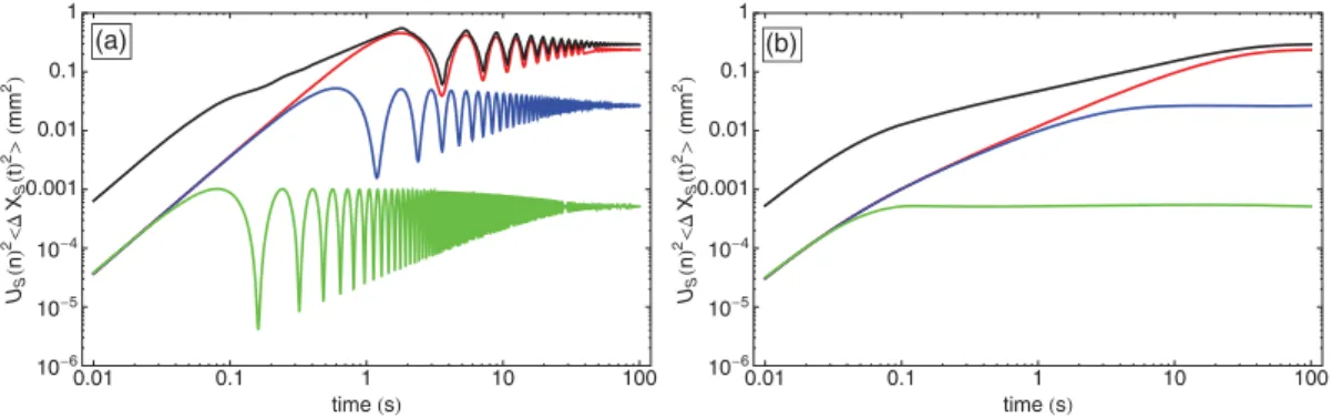
we plot in Fig.13the time evolution of the contributions of the modes s = 1, 3 and 33 for the center particle (n = 0). Two dampings are considered: γ = 0.1 s−1 [Fig.13(a)] and
γ = 60 s−1 [Fig. 13(b)]. The complete MSD curves, that include the contributions of all modes, are also displayed in order to discuss their main behaviors.
At very low damping, all modes oscillate before reaching their constant value [Fig. 13(a)]. The time evolution of %%u(n,t)2& in the intermediate regime is explained by the progressive disappearance in the sum(6)of the contributions of the modes s as soon as they lose their initial quadratic dependence with t. The power series development of %%X2
s(t)&
shows that it happens at a characteristic time t ≈ 2√3/ωs.
Thus at a given time t, the variation of %%u(n,t)2& with
time is dominated by the contributions of the modes such as t <2√3/ωs(strictly speaking, t < 2
√
3/(ω2s− γ2/4, which is the same for small γ ). The number P (t) of those modes may easily be estimated in the frame of the Debye approximation
P(t) ∼ 4 √
3N π√KD/M t
, (7)
where KD is an effective stiffness such that the dispersion
relation at small frequencies reads ωs = ) π 2N & KD M * s. (8)
The use of the Debye approximation is supported by the fact that the most important contributions in (6) come from the low frequencies, which follow a linear dispersion law. In the ballistic regime, each mode s behaves as %%X2
s(t)& ∼
kBT t2/M, and using(7)we obtain the MSD for the particle n
0.01 0.1 1 10 100 106 105 104 0.001 0.01 0.1 1 time s US n 2 XS t 2 mm 2 (a) (b) 0.01 0.1 1 10 100 106 105 104 0.001 0.01 0.1 1 time s US n 2 XS t 2 mm 2
FIG. 13. (Color online) Plot of the variations with time (in s) of the contribution %%X2
s(t)&Us(0)2of the mode s = 1 (red; dark gray, top),
s= 3 (blue; medium), s = 33 (green; bottom) to the MSD %%u(0,t)2& (in mm2) for a system of 33 particles and a SW confining potential with
5 10 15 20 25 30 0.0 0.2 0.4 0.6 0.8 1.0 P P, n (a) (b) 5 10 15 20 25 30 0.0 0.2 0.4 0.6 0.8 1.0 P P, n
FIG. 14. (Color online) Plot of the partial sum +(P ,n) as a function of P for particles n = ±15 (red dots), n = ±14 (blue squares), and n= 0 (green diamonds). (a) SW confining potential with λw= 1 mm and Ew/E0= 0.1. (b) LR confining potential with λw= 30 mm and
Ew/E0= 0.1. as %%u(n,t)2& ≈ + kBT M P(t) ' s=1 Us2(n) , t2= 2Dt. (9) In the opposite limit of very large damping, all modes are overdamped [Fig.13(b)] and evolve linearly as [2kBT /(Mγ )]t
before reaching saturation at a typical time γ /ω2
sfor the mode s
[13]. Now, the time evolution of %%u(n,t)2& is explained by the
progressive disappearance in the sum(6)of the contributions of the modes s when they reach their saturation. Thus, the modes that contribute to the variation of %%u(n,t)2& satisfy
t < γ /ω2s. Using once again the Debye approximation, the number P (t) is estimated as
P(t) ∼ 2N
π√KD/Mγ
√
t. (10)
Using(10), the expression of the MSD of the particle n is given by %%u(n,t)2& ≈ + 2kBT Mγ P(t) ' s=1 Us2(n) , t= F√t . (11) At this point, it is convenient to introduce the partial sum +(P ,n) ≡#Ps=1Us2(n) and to calculate its evolution accord-ing to the number P of modes that are taken into account. Such sums associated to three different particles n are presented in Fig. 14(a) and Fig. 14(b) for SR and LR confinements respectively.
In the SR case, whatever the considered particle, the sum increases roughly linearly with P . Then, each mode contributes to the MSD, even if they all have a different weight. We get +(P ,n) = 1 for P = 2N − 1. Thus, for the SR case, we may write in first approximation +(P ,n) ≈ P /(2N − 1). The LR case is very different. Now, for a given particle and a given confinement, the sum is roughly linear with P until P = Pmax(n,λw,Ew) < (2N − 1) and then jumps
abruptly to 1, which means that all modes of higher index do not contribute. This is due to the smallness of amplitudes Us(n) associated with high-frequency modes. Thus, as long
as P < Pmax(n,λw,Uw), the sum can be written as +(P ,n) =
+(Pmax,n)P /Pmax, and is equal to 1 otherwise. The evolution
of Pmax(n,λw,Ew) according to the particle index n for
different values of λw is shown on Fig.15. We see that Pmax
decreases with |n|.
Thus, in the case of small damping, all particles diffuse normally with %%u(n,t)2& = 2Dt with diffusion constants D
SR
and DLRrespectively associated with the SR and LR cases
DSR= 2 √ 3kBT N π(2N − 1)√MKD = 2√3kBT N π(2N − 1) & κ T Mρ, (12) DLR(n) = 2 √3k BT N π√MKD +(Pmax,n) Pmax(n,λw,Ew) = 2 √ 3kBT N +(Pmax,n) π Pmax(n,λw,Ew) &κ T Mρ, (13) where ρ is the mean particle density and κT = ρ/KD is
the isothermal compressibility, which takes into account the complete distribution of the stiffnesses in the chain.
At large damping, the MSD %%u(n,t)2& can be expressed
as F√t where the mobilities F are given, according to the confinement range, by:
FSR= 2kB T N π(2N − 1)√MKDγ = 2kBT π N 2N − 1 & κ T Mργ, (14) 0 5 10 15 0 5 10 15 20 25 30 index Pmax
FIG. 15. (Color online) Plot of Pmax(n,λw,Ew) as a function
of the particle index n for several LR confining potentials char-acterized by Ew/E0= 0.1 and λw= 4 mm (magenta triangles),
15 mm (black dots), and 30 mm (red diamonds). The values of Pmax(16,15 mm,0.1E0) and Pmax(16,15 mm,0.1E0) may be read in
FLR(n) = 4kB T N π√MKDγ +(Pmax,n) Pmax(n,λw,Ew) = 4kBπT N & κ T Mργ +(Pmax,n) Pmax(n,λw,Ew) (15)
Let us underline that the expressions DSR and FSR are
independent of the positions of the particles. Since the only parameter that depends on the confining force is KD, systems
in which the confinement results in the same equilibrium positions of the particles have the same set of diffusivities and mobilities. Those features are displayed in the simulation results for the HW and the SW cases (see Fig.1and Fig.2). In contrast, DLR(n) and FLR(n) explicitly depend on the index
of the particles n because of Pmax(n,λw,Ew). Both increase
as the particle gets closer to the walls, the highest coefficients being associated with the outermost particles. Moreover, the dependence of the diffusivities and mobilities on the effective stiffness KD indicates that they result from a collective effect.
Lastly, note also that they are proportional, with D/F = √γ /3. It means that, for a given set (λ
w,Ew), the mobility
scales as γ−1/2. This is indeed observed in the simulations,
as shown in Fig. 6. As an example, for λw= 15 mm and
Ew/E0= 0.1 the mobility is 0.07 mm2s−1/2 for γ = 10 s−1
and 0.03 ≈ 0.07/√6 mm2s−1/2 for γ = 60 s−1 as indicated
by Eq.(15).
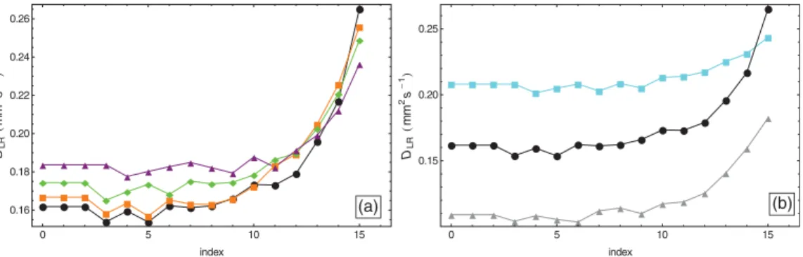
In Fig.16, the diffusivities given by the expressions(13)
are plotted as a function of the index for various values of the confinement length [Fig. 16(a)] and amplitude [Fig. 16(b)]. Those values are to be compared to the simulation data presented in Fig.4. We see that the simple estimates of Eqs.
(12)and(13)catch all qualitative features of the simulation data, such as the shape of the curves and their ordering with λw [Fig. 4(a)] and with Ew/E0 [Fig. 4(b)]. Quantitatively,
our estimates are in satisfactory agreement. Moreover, the mobilities may be directly calculated from the Fig. 16, multiplying by √γ /3. When compared with the mobility data displayed in Fig.6, we see that all qualitative features of the simulation data are recovered. The order of magnitude for the mobilities deduced from Fig.16 compare well with the simulations.
C. Crossover times
The correlation time tcorr(n), which characterizes the
begin-ning of the intermediate regime of a particle n is roughly given by 2√3/-ω2Pmax(n)− γ2/4 (for the sake of readability, the dependency of Pmaxupon λwand Ewis not written explicitly
in this section).
For the SW confinement case, most particles have Pmax(n) > 20. Since at large s the frequencies vary slowly with
the mode number (see Fig.10), their resulting correlation times are roughly the same. As the particle gets towards the wall, its frequency ωPmax(n) decreases and consequently its correlation
time is somewhat longer. In the HW case, all the Pmax(n) are
shifted towards larger s, thus tcorr(n) remains independent of
the particle position but, since their frequencies are smaller than in the SW case, the resulting value of the correlation time tcorr(n) is somewhat higher. However this concerns the inner
particles only. Indeed, the frequencies associated to Pmaxfor
the outermost particles correspond to localized modes with higher frequencies, so these particles have a smaller tcorr.
In the LR case, all the Pmax(n) are shifted toward the small s
and the high-frequency modes do not contribute efficiently to the MSD. This induces larger correlation times than in the SR cases, in particular for the outer particles for which the Pmax
are the most shifted. The evolution of the correlation times according to the particle positions for several values of λwand
Ew are shown in Fig.17. All these theoretical results are in
good agreement with the correlation times measured from the simulations (see Fig.7). Notice in particular that the change of evolution with λwobserved as the particle gets closer to the
wall is consistent with our theoretical estimates. In the case of hard-core interactions [6,28,29] this correlation time depends only on the particle concentration because the particles are free, except the direct contact with one of their neighbors. In the present situation, the particles are not actually free for t < tcorr
since they diffuse in the local potential of their neighbors and the walls, which explains why tcorrdepends on the interactions.
After the intermediate regime, the saturation time for the particle n is controlled by the frequency of the mode s= Pmin(n,λw,Uw). As before, we do not write explicitly the
dependency of Pminupon λwand Uwin the rest of this section.
When ωPmin> γ /2, most modes are oscillating ones as shown
by Fig. 13(a). Thus, the saturation time may be estimated from Eq. (5) by π(ω2
Pmin− γ
2/4)−1/2. On the other hand, if
0 5 10 15 0.16 0.18 0.20 0.22 0.24 0.26 index DLR mm 2s 1 (a) (b) 0 5 10 15 0.15 0.20 0.25 index DLR mm 2s 1
FIG. 16. (Color online) Plot of the theoretical diffusivities (in mm2s−1) as a function of the particle index n. (a) E
w/E0= 0.1, λw= 4
mm (magenta triangles), 7 mm (green diamonds), 11 mm (orange squares), and 30 mm (red dots). (b) λw= 15 mm, Ew/E0= 0.005 (cyan
2 4 6 8 10 12 14 16 0.07 0.08 0.09 0.10 0.11 index tcorr s 0 5 10 15 0.04 0.05 0.06 0.07 0.08 0.09 0.10 index tcorr s (a) (b)
FIG. 17. (Color online) (a) Theoretical correlation times tcorr(s) as a function of the particle index n. (a) Ew/E0= 0.1; λw= 4 mm (magenta
triangles), 7 mm (green diamonds), 15 mm (black dots). (b) λw= 15 mm; Ew/E0= 0.005 (magenta circles), 0.1 (black dots), and 0.5 (gray
triangles).
ωPmin< γ /2, the modes are overdamped [see Fig.13(b)] and
the saturation time is π[γ /2 − (ω2 Pmin− γ
2/4)1/2]−1. At very
large damping, this time is πγ /ω2
Pmin. At very small damping,
the saturation time is π/ωPminfor all particles. Since ωPmin(n) is
roughly equal to ωPmaxN/(N−n), the saturation time decreases
linearly with n. In the intermediate γ range, the outer particles with the highest ωPmin could be in the small damping regime
while the inner ones with smaller ωPminare in the large damping
regime. Thus, the saturation times are independent of γ for the outer particles but strongly depend on the damping for the inner ones, and the evolution of tsat according to the index
n shows a jump at the particle, which corresponds to this change of regime. This analysis is in complete agreement with the behaviors observed in the simulations (see Fig.8). The intermediate regime extends between tcorrand tsat, respectively,
determined by the frequencies associated with Pmax and
Pmin. However, the amplitude |Us(±16)| corresponding to the
contribution of the mode s to the motion of the outermost particles presents a maximum for only one mode s, as shown by Fig.11. Therefore, tcorr= tsat, which explains the absence
of intermediate regime for those particles.
D. Saturation unevenness
The behavior of the normal modes also explains the unevenness observed in the saturation regime and the evolution of its value according to λw and Ew. This unevenness exists
only when the damping is small enough for the mode s = 1 to be an oscillating mode. It corresponds to the first local minimum in the time evolution curve of the mode s = 1, which is typically reached at t = 2π(ω2
1− γ2/4)−1/2. For
a mode s > 1 whose frequency is proportional to ω1, this
time also corresponds to its sth minimum (this is true at low frequencies, associated to the main contributions, since the dispersion relation is linear). The unevenness is then explained by the superposition at the same time of all these minima and its time position is independent of the particle considered. This surperposition also exists in the case of cyclic systems, but the unevenness is masked by the translationally invariant mode, which evolves linearly in time and dominates the dynamic at long time [13]. When λwor Ewincrease, the unevenness shifts
towards short times since ω1 increases (see Fig.10). On the
contrary, when γ increases, the unevenness shifts towards long
times. Thus, the unevenness depth δdepthmay be estimated as
δdepth≈ ' s $ Us2(n)e−γ π/ω1 ω2s− γ2/4 % . (16)
It increases from the outermost particle to the central one and decreases with γ , in perfect agreement with the simulation results (see Figs.1–3).
E. Discussion
All the behaviors obtained with these theoretical expres-sions are in perfect agreement with the simulation results; they also explain the experimental observations presented in Ref. [13]. The analysis of the equilibrium positions obtained in these experiments shows that the decrease of the applied voltage V is equivalent to a displacement of the (λw,Ew) point
inside the LR domain. The observed increase of diffusivity D as the voltage V decreases is explained by the relation
(13), as well as its increase with the particle index |n|. In the same way, our analysis explains the observed mobilities, which were left unexplained in Ref. [27] but are consistent with(15)
(see Fig 10 of Ref. [27]. There is a misprint in the caption where the colors have been transposed. The text in the body of the paper is correct). In this article, we also presented a surprising result concerning the correlation time. While the correlation time measured for V = 1300 V is always higher than the one measured at 1000 V, the opposite is observed for the outermost balls (see Fig 8. of Ref. [27]). This is in agreement with our estimations of the correlation time displayed in Fig.17.
V. CONCLUSION
We have described the SFD of a finite number of particles with soft-core interactions, confined in a linear and finite box and submitted to thermal fluctuations. We have performed numerical simulations of the relevant Langevin equations and proposed to describe this system as a chain of linear springs and point masses in a thermal bath. In a previous work [30], we have identified three different kinds of confinement, according to the relative values of the springs: The SR confining forces are such that interparticle interactions may be described by identical springs, with HW and SW confining forces corresponding to a wall-particle interaction respectively higher and smaller than the interparticle interactions. For the
LR confinement the springs vary along the line. Since such systems have finite size, the particles’ MSD reach constant values at very long times (tsat! t). In a previous article, we
have studied the effects of the confinement on the MSD in this saturation regime [30]. Here we focus on the transient behaviors at short times.
Two regimes have been identified for the transient time evolution of the MSD %%u(n,t)2& of the nth particle. At small
times (0! t ! tcorr), it evolves as %%u(n,t)2& = (kBT /m)t2.
This is a ballistic flight that results from the inertial effects and is observed whatever the damping γ , the particle n, and the confinement range. For (tcorr! t ! tsat), an intermediate
regime takes place in which the power law describing the evolution of the MSD according to the time depends on the damping value. For small damping, a linear scaling in t is observed and a constant diffusivity may be defined for all the particles. For large damping, the MSD undergoes a SFD scaling in t1/2 and mobilities may be determined. In these
finite-size linear systems, the translation invariance is broken and the evolution of the MSD according to the time depends on the rank of the particle in the line.
We exhibit a strong dependency of the dynamics on the confinement. While the dynamic of the outermost particles is the slowest in the HW case, it is by contrast the fastest in the SW and LR cases. Moreover, while the behavior of the MSD may be described by a single diffusivity or a single mobility in the case of a SR confinement, these coefficients
vary along the line for a LR confinement. In this case, both coefficients increase when the considered particle is far from the confining walls. The crossover times depend on the confinement too. For LR confinement, the correlation times strongly increase for particles close to the wall whereas the saturation times decrease as the particle gets farther from the walls.
From a theoretical point of view, we show that the motion of the particles of such systems may be described in terms of the normal modes of oscillation of the corresponding chain of springs and point masses. The MSD results from the superposition of all these modes, which undergo the same dynamic as an oscillator in an harmonic well. The overdamped modes, which do not oscillate until they saturate, contribute to the SFD scaling in t1/2. The underdamped modes oscillate
before reaching their saturation and contribute to the linear time scaling. The particularity of finite-sized linear systems is that the particles are not equivalent. Each of them is associated with specific modes in which they oscillate preferentially. Thus, the superposition of modes is different for each particle. Complete expressions of their diffusivities and mobilities have been expressed according to the relevant parameters. Those estimates are in perfect agreement with our simulation data. With this model, we recover the correct power laws for the time dependency of the MSD in the various regimes, and we are able to estimate the prefactors according to the relevant parameters.
[1] D. Jepsen,J. Math. Phys.6, 405 (1965). [2] R. Arratia,Ann. Prob.11, 362 (1983).
[3] P.-G. de Gennes,J. Chem. Phys.55, 572 (1971). [4] D. G. Levitt,Phys. Rev. A8, 3050 (1973). [5] P. M. Richards,Phys. Rev. B16, 1393 (1977).
[6] H. van Beijeren, K. W. Kehr, and R. Kutner,Phys. Rev. B28, 5711 (1983).
[7] J. K¨arger,Phys. Rev. A45, 4173 (1992).
[8] K. Hahn and J. K¨arger,J. Phys. A28, 3061 (1995). [9] K. Hahn and J. K¨arger,J. Phys. Chem. B102, 5766 (1998). [10] A. Taloni and F. Marchesoni,Phys. Rev. E74, 051119 (2006). [11] M. Kollmann,Phys. Rev. Lett.90, 180602 (2003).
[12] B. Felderhof,J. Chem. Phys.131, 064504 (2009).
[13] J.-B. Delfau, C. Coste, and M. Saint Jean,Phys. Rev. E84, 011101 (2011).
[14] T. Ooshida, S. Goto, T. Matsumoto, A. Nakahara, and M. Otsuki, J. Phys. Soc. Jpn.80, 074007 (2011).
[15] B. Lin, M. Meron, B. Cui, S. A. Rice, and H. Diamant,Phys. Rev. Lett.94, 216001 (2005).
[16] V. Borman, B. Johansson, N. Skorodumova, I. Tronin, V. Tronin, and V. Troyan,Phys. Lett. A359, 504 (2006).
[17] Q.-H. Wei, C. Bechinger, and P. Leiderer,Science 287, 625 (2000).
[18] B. Lin, B. Cui, J.-H. Lee, and J. Yu,Europhys. Lett.57, 724 (2002).
[19] C. Lutz, M. Kollmann, P. Leiderer, and C. Bechinger,J. Phys.: Condens. Matter16, S4075 (2004).
[20] G. Coupier, C. Guthmann, Y. Noat, and M. Saint Jean,Phys. Rev. E71, 046105 (2005).
[21] G. Coupier, M. Saint Jean, and C. Guthmann,Phys. Rev. E73, 031112 (2006).
[22] G. Coupier, M. Saint Jean, and C. Guthmann,Europhys. Lett. 77, 60001 (2007).
[23] C. Coste, J.-B. Delfau, C. Even, and M. Saint Jean,Phys. Rev.
E81, 051201 (2010).
[24] K. Nelissen, V. Misko, and F. Peeters,Europhys. Lett.80, 56004 (2007).
[25] S. Herrera-Velarde and R. Casta˜neda-Priego,J. Phys.: Condens. Matter19, 226215 (2007).
[26] L. Lizana, T. Ambjornsson, A. Taloni, E. Barkai, and M. A. Lomholt,Phys. Rev. E81, 051118 (2010).
[27] J.-B. D. Delfau, C. Coste, C. Even, and M. Saint Jean,Phys. Rev. E82, 031201 (2010).
[28] L. Lizana and T. Ambj¨ornsson,Phys. Rev. Lett.100, 200601 (2008).
[29] L. Lizana and T. Ambj¨ornsson,Phys. Rev. E80, 051103 (2009). [30] J.-B. Delfau, C. Coste, and M. Saint Jean, Phys. Rev. E85,
041137 (2012).
[31] S. Herrera-Velarde and R. Casta˜neda-Priego,Phys. Rev. E77, 041407 (2008).
[32] B. Cui, H. Diamant, and B. Lin,Phys. Rev. Lett.89, 188302 (2002).
[33] C. Lutz, M. Kollmann, and C. Bechinger,Phys. Rev. Lett.93, 026001 (2004).
[34] M. K¨oppl, P. Henseler, A. Erbe, P. Nielaba, and P. Leiderer, Phys. Rev. Lett.97, 208302 (2006).
[35] P. Henseler, A. Erbe, M. K¨oppl, P. Leiderer, and P. Nielaba, Phys. Rev. E81, 041402 (2010).

![FIG. 3. (Color online) Plot of MSD % %u(n,t) 2 & (in mm 2 ) as a function of time (in s), for a system of 33 particles and a LR confining potential with E w = 0.1E 0 and λ w = 4 mm [(a) and (d)], λ w = 11 mm [(b) and (e)], and λ w = 30 mm [(c) and (f)]](https://thumb-eu.123doks.com/thumbv2/123doknet/14604122.544351/6.911.85.825.103.813/fig-color-online-plot-function-particles-confining-potential.webp)