HAL Id: hal-00350211
https://hal.archives-ouvertes.fr/hal-00350211
Submitted on 6 Jan 2009HAL is a multi-disciplinary open access
archive for the deposit and dissemination of sci-entific research documents, whether they are pub-lished or not. The documents may come from
L’archive ouverte pluridisciplinaire HAL, est destinée au dépôt et à la diffusion de documents scientifiques de niveau recherche, publiés ou non, émanant des établissements d’enseignement et de
Projective topology on bifinite domains and applications
Samy Abbes, Klaus Keimel
To cite this version:
Samy Abbes, Klaus Keimel. Projective topology on bifinite domains and applications. Theoretical Computer Science, Elsevier, 2006, 365 (3), pp.171-183. �10.1016/j.tcs.2006.07.047�. �hal-00350211�
Projective Topology on Bifinite Domains and
Applications
Samy Abbes
a,1a
LIAFA – Universit´e Paris 7
Klaus Keimel
bb
Technische Universit¨at Darmstadt
Abstract
We revisit extension results from continuous valuations to Radon measures for bifi-nite domains. In the framework of bifibifi-nite domains, the Prokhorov theorem (exis-tence of projective limits of Radon measures) appears as a natural tool, and helps building a bridge between Measure theory and Domain theory. The study we present also fills a gap in the literature concerning the coincidence between projective and Lawson topology for bifinite domains. Motivated by probabilistic considerations, we study the extension of measures in order to define Borel measures on the space of maximal elements of a bifinite domain.
Key words: Bifinite domains, Continuous valuations, Radon measures, Maximal elements
1 Introduction
A recent research area concerns so-called probabilistic concurrent systems [16,1]. The main problem is to describe and study, a random behavior of systems with concurrency properties. Engineering applications of this topic are found in the study of large distributed systems, such as telecommunication networks [3]. Probabilistic extensions have been developed for some models from Concur-rency theory, in particular for Winskel’s event structures and for 1-bounded Petri nets. The domain of configurations of an event structure represents the
1
different processes that can occur in the system modeled by the event struc-ture. In turn, the maximal elements of the domain represent the complete his-tories, or runs of the system. According to the usual concepts from stochastic processes theory, a probabilistic event structure, seen as a model of concurrent probabilistic system, is thus specified by a probability measure on the space of runs of the system, i.e., on the space of maximal elements of its domain of configurations. It is understood that the σ-algebra that equips the space of maximal configurations is the Borel σ-algebra related to some topology of the domain, for instance, the Borel σ-algebra associated with the Lawson topol-ogy. This setting encompasses of course systems without concurrency, such as discrete Markov chains, where the maximal elements of the domain are the infinite sequences of states of the chain.
Hence, the notion of concurrent probabilistic system is conceptually not very different from other “classical” probabilistic systems, and is not even particular to event structures. A general concurrent probabilistic system can be defined as a probability measure on the space of maximal elements of some Dcpo. We will explain below why this definition suffers from too much generality to be useful in practice.
The next step in the theory of probabilistic concurrent systems is to explicitly specify a probability measure on the space of maximal elements of a Dcpo. This is usually decomposed, at least for classical stochastic processes, in two steps:
(1) Specify a probability for finite processes of the system, if possible in an incremental fashion (for instance, the chain rule for discrete Markov chains); this is the central job of probability theory [1].
(2) “Extend” the probabilistic behavior of finite processes to a probability measure on the space of maximal elements; this requires a measure-theoretic argument.
It turns out that, for concurrent systems, both steps 1 and 2 above are more difficult than for non-concurrent systems, such as Markov chains. The issues encountered when dealing with concurrency models have led one of the au-thors to study a restricted class of event structures, in particular for step 1, the so-called locally finite event structures [1]. Other authors have studied the even more restrictive class of confusion-free event structures [16]. In the study of locally finite event structures, the extension measure-theoretic argument used was Prokhorov extension theorem for projective systems of probabilities. This solution has several advantages: besides its simplicity and elegance, it provides an effective way to describe the probability measure on the space of maximal configurations by means of a (countable) collection of finite probabil-ity measures. It is therefore very attractive to extend this method to models more general than event structures.
A natural class of domains that could be used for extension results of this kind is the class of bifinite domains thanks to their representation as projective lim-its of finite posets. Bifinite domains have been introduced by Plotkin [15] in the countably based case as projective limits of sequences of finite posets and by Gunter [7] and Jung [10] in the general case. The class of bifinite domains encompasses the domains of configurations of Winskel’s event structures. Bifi-nite domains have encountered a particular interest since their category is Cartesian closed [6].
This paper aims to present extension results for bifinite domains. We do not restrict ourselves to the extension problem on the space of maximal elements of bifinite domains, but also revisit the problem of the extension of a continuous valuation on the domain to a Radon measure on the domain. For this, we propose a self-contained study of bifinite domains exclusively based on their projective representation. The extension of measures on the space of maximal elements appears as a byproduct of this study, although it was one of our original motivations.
More specifically, we prove the following results: the projective topology of the domain coincides with its Lawson topology (Theorem 1); there is a one-to-one correspondence between continuous valuations on a bifinite domain, and Radon measures on the domain equipped with the Borel-Lawson σ-alge-bra (Theorem 2); the space of maximal elements of a bifinite domain can be represented as a projective limit of finite sets if and only if the space is compact for the Lawson topology (Theorem 3). Theorem 1 is certainly known by specialists, although we are not aware of its explicit formulation in the literature. On the one hand, Theorem 2 is known for more general cases than for bifinite domains [2,12]. On the other hand the proof we give here is new; it uses the Prokhorov theorem on projective limits of measures; the proof is more direct than in [2], and makes clearer the use of the measure-theoretic argument. The problem of extension of continuous valuations to Borel measures has been popularized by Lawson [13]. Finally, Theorem 3 gives a fundamental limitation for the representation of a measure on the space of maximal elements of a bifinite domain as a projective limit of measures of finite sets.
The paper is organized as follows: Section 2 collects the needed background on projective limits and bifinite domains. To keep the paper self-contained we have given proofs of most of the results, that are usually presented as corollaries of results in more general frameworks than bifinite domains. We also there state the coincidence between the projective and the Lawson topologies on bifinite domains. Then we apply this result to the extension of continuous valuations to Radon measures in Section 3, and study the representation of the space of maximal elements as a projective limit of finite sets in Section 4.
2 Background
2.1 Dcpos
We recall some elements from Domain theory (see [6]). The aim is to quickly arrive to the definition of bifinite domains, that will constitute our main model. We assume basic knowledge on posets (partially ordered sets). If X is a subset of a poset (L, ≤), we denote by sup X the least upper bound (l.u.b.) of X in L, if it exists. We most usually denote a poset (L, ≤) simply by L when no confusion occurs on the ordering relation involved. For a poset L, the downward closure ↓a and the upward closure ↑a of an element a ∈ L are defined to be:
↓a = {x ∈ L : x ≤ a}, ↑a = {x ∈ L : a ≤ x}.
Let L be a poset. A subset D ⊆ L is said to be directed, if it is nonempty and if any two elements x, y ∈ D have a common upper bound in D. A Dcpo (directed complete poset) is a poset L every directed subset of which has a l.u.b. in L.
Let L, M be two posets. A mapping f : L → M is said to be order preserving if f (x) ≤ f (x′) for any two elements x ≤ x′ in L. If M is a Dcpo, the image
f(D) of any directed set D under such a mapping f is a directed set. This makes the following definition meaningful: if L, M are two Dcpos, a mapping f : L → M is said to be Scott-continuous if f is order preserving, and if sup(f (D)) = f (sup(D)) for any directed set D ⊆ L.
2.2 Projective Limits of Sets, Posets and Spaces
Let (Li)i∈I be a family of sets. We denote by:
L=Y
i∈I
Li,
the product of the the family (Li)i∈I, the elements of which are all families
(li)i∈I such that li ∈ Li for each i ∈ I. We denote by πi : L → Li the canonical
projections.
Assume that I is equipped with some ordering ≤, such that I is directed. We assume that, for each pair i ≤ j in I, we are given mapping gij : Lj → Li,
such that the following equalities hold:
∀i, j, k ∈ I, gii= IdLi, i≤ j ≤ k =⇒ gik = gij ◦ gjk.
The data³(Li)i∈I,(gij)i≤j in I
´
is called a projective system. The mappings gij
are called the bonding maps. The family (gij)i≤j in Iis most usually understood,
so that we denote the projective system simply by (Li)i∈I. The projective limit
of the projective system (Li)i∈I is defined to be the following subset D of L:
D=n(li)i∈I ∈ L : ∀i ≤ j in I, li = gij(lj)
o
.
We denote by gi : D → Li the restriction to D of the projection πi : L → Li,
for i ∈ I. The following identities hold:
∀i ≤ j in I, gi = gij ◦ gj. (1)
Assume that each Li is equipped with an ordering. Then the product L is
equipped with the product ordering:
∀(l, l′) ∈ L × L, l ≤ l′ ⇐⇒ ∀i ∈ I, π
i(l) ≤ πi(l′).
Then (L, ≤) is a partial order, and every projection πi : L → Li is order
pre-serving. Moreover, if each Li is a Dcpo, then L is a Dcpo and the projections
πi : L → Li are Scott-continuous.
The projective limit D of a projective system built upon the family (Li)i∈I
with order preserving bonding maps gij, i≤ j, is equipped with the ordering
induced from L by restriction. The maps gi : D → Liare then order preserving.
If the Li are Dcpos, and if the bonding maps are Scott-continuous, then D is
a Dcpo and the mappings gi : D → Li are Scott-continuous.
Finally, instead of an ordering, consider a topology τi on each of the sets Li.
The product L is equipped with the product topology τ . This is the coarsest topology rendering continuous all the canonical projections πi. A subbasis for
the open sets of this topology is given by the sets of the form π−1i (U ) where i ∈ I and U ∈ τi.
It suffices indeed to choose the open sets U in some subbase for the topology τi.
The projective limit D of a projective system built upon the family (Li)i∈I
of topological spaces with continuous bonding maps gij, i ≤ j, is equipped
with the topology induced from the product topology on L by restriction. The maps gi : D → Li are then continuous.
2.3 Projection-embedding pairs. Bifinite domains
Let L and M be two posets. Let d : L → M and g : M → L be two functions. We say that (g, d) is a projection-embedding pair if both g and d are order preserving, and if moreover:
d◦ g ≤ IdM , g◦ d = IdL . (2)
g is called the upper adjoint and d is called the lower adjoint. As the lower adjoint d is uniquely determined by the upper adjoint g, if it exists [6, O-3.2], we may denote it by d = ˆg. We say that g is a projection, if it is order preserving and if there is a lower adjoint d such that (g, d) is a projection embedding pair. By (2), projections are surjective and their lower adjoints are order embeddings. A projection-embedding pair is a particular case of an adjunction pair (see [6, O-3.1]). We recall the following properties of adjunction pairs (g,g):b
(A1) [6, O-3.1] For elements s ∈ M and t ∈ L, one has g(s) ≥ t if and only if s ≥bg(t); in other words: g−1(↑t) = ↑bg(s).
(A2) [6, O-3.3] bg is Scott-continuous.
(A3) Projection-embedding pairs compose: if (g,g) and (f,b fb) are two projection-embedding pairs as shown in the left diagram below, then the composite (g ◦ f,fb◦g) in the diagram at right is also a projection embedding-pair:b
L b g // M g oo b f // N f oo , L b f ◦bg // N g◦f oo
We will be interested in projective systems (Li)i∈I of Dcpos with
Scott-continuous projections gi,j, i ≤ j, as bonding maps, and their projective
limit D.
Note that, thanks to property (A3), the identity gik = gij ◦ gjk for i ≤ j ≤ k
implies the contravariant identity
b
gik =gbjk ◦bgij (3)
on lower adjoints. We have the following result which, informally speaking, says that we can make k → ∞ in the above equation:
Lemma 1 Let D be the projective limit of a projective system of Dcpos (Li)i∈I with Scott-continuous projections gij as bonding maps. Then the
fol-lowing properties hold:
(1) for each i ∈ I, the canonical map gi : D → Li is a Scott-continuous
projection and has a lower adjoint bgi;
(3) for each y ∈ D, the family yi =gbi◦ gi(y), i ∈ I is a directed subset of D,
and supiyi = y.
Proof. 1. Let i0 ∈ I, and x ∈ Li0. We define an element (xi)i∈I in the product
Q
i∈ILi as follows: For each i ∈ I, let p ∈ I such that p ≥ i and p ≥ i0. Such
a p exists since I is directed. Then we put xi = gip◦gbi0p(x). We claim that
xi does not depend on the choice of p. Indeed, let q ∈ I be another common
upper bound of i, i0, and let x′i = giq ◦gbi0q(x) . Pick r ∈ I such that r ≥ p, q.
Such an r exists since I is directed; the following diagram represents the posets involved: Lr Lp Lq Li Li0 ¡¡ ¡ ✒ ❅ ❅ ❅ ■ ✻ ✟✟✟✟ ✟✟✟✟ ✯ ✻ ❍ ❍ ❍ ❍ ❍ ❍ ❍ ❍ ❨
where the arrows represent the lower adjoints of bonding maps. The diagram commutes thanks to Equation (3). By definition, we have the identity gpr◦gbpr =
IdLp, whence:
xi = gip◦gbi0p(x) = gip◦ (gpr ◦gbpr) ◦gbi0p(x) = gir◦gbi0r(x).
For the same reasons we have:
x′i = giq ◦bgi0q(x) = giq◦ (gqr◦gbqr) ◦gbi0q(x) = gir◦gbi0r(x).
Therefore xi = x′i as claimed. Moreover, the element (xi)i∈I belongs to the
projective limit D. Indeed, let i ≤ j, we have to show:
gij(xj) = xi. (4)
For this, pick p ∈ I such that p ≥ j, i0. Then we also have p ≥ i. Therefore
xi = gip◦gbi0p(x) and xj = gjp◦bgi0p(x). Hence:
gij(xj) = (gij ◦ gjp) ◦gbi0p(x) = gip◦gbi0p(x) = xi.
which proves (4). We consider thus the mappinggbi0 : Li0 → D defined by x ∈
Li0 7→gbi0(x) = (xi)i∈I, and we prove that (gi0,gbi0) is a projection-embedding
pair. It is clear from the definition thatgbi0 is order preserving, and we already
know that gi0 is order preserving. It is also clear that gi0 ◦gbi0 = IdLi0. It
remains thus only to show:
For this, we claim first that, if z = (zi)i∈I and y = (yi)i∈I are two elements
of D, then:
z ≤ y ⇐⇒ ∃k ∈ I : ∀i ∈ I, i≥ k ⇒ zi ≤ yi. (6)
We prove this claim. The (⇒) part is trivial. For the converse implication, assume there exists k ∈ I as in (6). For each i ∈ I, there is a j ∈ I such that j ≥ i and j ≥ k since I is directed. Then zj ≤ yj, and since gij is order
preserving, this implies zi = gij(zj) ≤ gij(yj) = yi. Hence z ≤ y, and the claim
is proved.
We now come back to (5). Let x ∈ Li0 and let y = (yi)i∈I be an element
of D. If gbi0(x) ≤ y, then since gi0 is order preserving and by the identity
gi0◦bgi0 = IdL0, this implies that x ≤ gi0(y), which proves the (⇐) part of (5).
Conversely, assume that x ≤ gi0(y), and let z = gbi0(x). Then, by definition
ofgbi0, we have zi =gbi0i(x) for any i ∈ I such that i ≥ i0. Hence, for any i ≥ i0,
we have:
zi =gbi0i(x) ≤bgi0i(yi0) = gbi0i◦ gi0i(yi) ≤ yi,
where the last inequality comes from property (A2) above. Therefore, thanks to (6), we conclude that z =gbi0(x) ≤ y, which completes the proof of (5). We
have obtained so far that (gi0,gbi0) is a projection-embedding pair.
2. From the identity gi = gij◦ gj, valid for i ≤ j, we obtain thanks to (A3) by
taking the lower adjoints bgi =gbj ◦bgij.
3. Denote fi = bgi ◦ gi for each i ∈ I. Fix y ∈ D. Observe first that fi(y) ≤
fj(y) if i ≤ j. Indeed, fi(y) = bgj ◦ (bgij ◦ gij) ◦ gj(y) by point 2 above. Since
b
gij ◦ gij ≤ IdLj by property (A1) of projection-embedding pairs, it follows
that fi(y) ≤gbj ◦ gj(y) = fj(y), as claimed. Since I is directed, it follows that
yi = fi(y), i ∈ I, is a directed subset of D. Now we show that supiyi. On
the one hand, y ≥fbi(y) for all i ∈ I by property (A1). On the other hand, if
z ∈ D is such that z ≥ fi(y) for all i ∈ I, then gi(z) ≥ gi(y) for all i ∈ I by the
definition of adjunction pairs. In other words, z ≥ y in D. Hence, y = supyyi.
✷
It is appropriate now to recall the notions of compact elements and algebraic domains:
Definition 1 An element k of a Dcpo D is called compact, if the following property holds: whenever X is a directed subset of D such that sup X ≥ k, then there is an element x ∈ X such that x ≥ k. A Dcpo D is called algebraic, if for each of its elements x there is a directed set K of compact elements such that x = sup K.
These properties of domains are preserved under projective limits. First we state the following lemma (see [6, Exercise I-4.34]):
Lemma 2 Let g : C → D be a Scott-continuous projection map of Dcpos and gb: D → C its lower adjoint. Then an element k ∈ D is compact in D if and only if g(k) is compact in C.b
We now are ready for:
Lemma 3 Let D be the projective limit of a projective system (Li)i∈I of
alge-braic domains with Scott-continuous projections gi,j, i ≤ j, as bonding maps.
Let gbi : Li → D be the lower adjoints defined in Lemma 1, point 1. Then D is
an algebraic domain. An element y ∈ D is compact if and only if y = gbi(k)
for some i ∈ I and some compact element k ∈ Li.
Proof. Let y ∈ D be such that y = gbi(k) for some i ∈ I and some compact
element k ∈ Li. By the preceding lemma, y is compact. Conversely, let y be a
compact element of D. As y is the l.u.b. of the directed set gbi◦ gi(y), there is
an i ∈ I such that y =gbi◦ gi(y), whence y =gbi(x) with x = gi(y) ∈ Li. Again
by the preceding lemma, x is compact in Li. Thus, we have proved that the
compact elements y of D are of the form y =gbi(k) for some i ∈ I and some
compact element k ∈ Li.
In order to prove algebraicity of D, let y be an arbitrary element of D. We know that y is the l.u.b. of the directed familyg(xb i), where xi = gi(y) ∈ Li. As each
Li is supposed to be algebraic, there is a directed set Xi of compact elements
in Li such that xi = sup Xi. Then the set Y =Sig(Xb i) is a directed family of
compact elements in D such that sup X = supisupg(Xb i) = supigb(sup Xi) =
supigbi(x) = y. ✷
We now come to the main object of our paper:
Definition 2 Assume that I is a directed poset. A projective system (Li)i∈I,
with bonding maps gij for i ≤ j, is called a projective system of finite type if
all Li are finite posets, and if each bonding map gij : Lj → Li, for i ≤ j, is
a projection with lower adjoint gbij : Li → Lj. The projective limit of such a
projective system is called a bifinite domain.
As in a finite domain every element is compact, the preceding lemma has the following consequence:
Corollary 1 Let D be a bifinite domain, represented as the projective limit of a projective system (Li) of finite type with bonding maps gij. Then D is an
algebraic domain. An element y of D is compact if and only if y = gbi(x) for
2.4 Topologies
Several topologies can be defined on Dcpos, and in particular on bifinite domains. This subsection describes these topologies. It is one of the aims of the paper to describe their relationships.
Recall that a topology τ on a set X is said to be coarser than a topology σ on X if τ ⊆ σ. The topology generated by a family F of subsets of X is defined as the coarsest topology that contains all elements of F as open sets.
Scott, lower and Lawson topologies. A subset U of a Dcpo D is called Scott-open if:
(1) U is increasing; i.e.: ∀x ∈ U, ↑x ⊆ U ;
(2) (Scott condition) for any directed subset X of D, we have: sup X ∈ U ⇒ U ∩ X 6= ∅.
The collection of Scott-open sets is a topology on D called the Scott topology. The lower topology on a Dcpo D is the topology generated by the sets of the form D \ ↑x, with x ranging over D. Finally, the Lawson topology on D is the join of the Scott and of the lower topologies on D. We denote by σ, ω and λ the Scott topology, the lower topology, and the Lawson topology, respectively. For an algebraic domain D, the sets of the form ↑k for compact elements k ∈ D form a basis for the open sets of the Scott topology, and their complements D\ ↑k form a subbasis for the open sets of the lower topology.
On a finite set, the open sets for the Scott topology are the upper sets and the open sets for the lower topology are the lower sets. The Lawson topology is discrete.
Lemma 4 Let C and D be Dcpos and g : C → D a Scott-continuous pro-jection with lower adjoint gb: D → C. Then g is lower continuous, hence Lawson-continuous, and bg is an embedding for the respective Scott topologies.
Proof. By property (A3) characterizing adjunctions, the inverse image g−1(↑y)
is ↑gb(y). Thus the inverse image of a subbasic closed set for the lower topology on D is a subbasic closed set for the lower topology on C. This shows that bg is lower continuous.
As gb is Scott-continuous, it remains to show, that for any Scott-open set V in D, there is a Scott-open set U in C such that U ∩g(D) =b bg(V ). For V Scott-open in D, let U = Sv∈V ↑g(v). For x ∈ D withb bg(x) ∈ U there is a
v ∈ V such thatg(x) ≥b g(v) whence x = g(b g(x)) ≥ g(b g(v)) = v which impliesb
x ∈ V . Thus U ∩g(D) =b g(V ). It remains to show that U is Scott-open.b
By definition, U is an upper set. Let X be a directed subset of C such that sup X ∈ U . Then sup X ≥g(v) for some v ∈ V . As g is Scott-continuous, web
get sup g(X) = g(sup X) ≥ g(g(v)) = v ∈ V . As V is Scott-open, we concludeb
that there is an x ∈ X with g(x) ∈ V . We conclude thatg(g(x)) ≤ x, whenceb
x∈ U . ✷
Projective Topologies. Let D be an algebraic domain, defined as the pro-jective limit of a propro-jective system (Li)i∈I of algebraic domains with
projec-tions gij as bonding maps. We consider our three topologies on Dcpos, the
Scott topology, the lower topology and the Lawson topology, on all of the Li.
Let L be the product of the family (Li)i∈I. Each of the three topologies yields
a product topology on L and induces a topology on the subset D. We call it the associated projective topology, and it is the coarsest topology on L that makes all the projections gi : D → Li continuous. A subbasis for the open
sets of the product topology is given by the sets of the form gi−1(U ) where
gi: D → Li is any of the canonical projections and U a basic open set in Li.
Finally, for a bifinite domain D, we refer to the Lawson-projective topology simply with the expression projective topology. This is what is usually under-stood when talking about the projective topology of a projective limit of finite sets equipped with the discrete topology, as it is the case for bifinite domains. The Scott topologies on the Li yield a projective topology ˜σ on D. As a basis
for the Scott-open sets of the algebraic domains Li is given by the sets of the
form ↑x, where x is a compact element of Li, a subbasis for the open sets for
the topology ˜σ on L is given by the subsets of the form U = g−1
i (↑x), i∈ I, x∈ Li. (7)
As g−1
i (↑x) = ↑bg(x) by (A1) and as, by Corollary 1, the compact elements of
Dare precisely the images gbi(x) of compact elements in the Li, the projective
topology ˜σ coincides with the intrinsic Scott topology on the projective limit D.
The lower topologies on the Li yield a projective topology ˜ω on D. As a basis
for the lower closed sets of the algebraic domains Li is given by the sets of the
form ↑x, where x is a compact element of Li, a subbasis for the closed sets for
the topology ˜ω on L is given by the subsets of the form U = g−1
i (↑x), i∈ I, x∈ Li. (8)
As gi−1(↑x) = ↑bg(x) by (A1) and as, by Corollary 1, the compact elements of
topology ˜ω coincides with the intrinsic lower topology on the projective limit D.
The Lawson topologies on the Li yield a projective topology ˜λ on D. As the
Lawson topology is the join of the lower and the Scott topology, the projective topology ˜λ coincides with the intrinsic Lawson topology on D by the above. With respect to the Lawson topology, an algebraic domain is always a Haus-dorff space. Thus, on L = QiLi, the product of the Lawson topologies is
Hausdorff, too. We claim that the projective limit domain D is a closed sub-set in L: Indeed D can be described as follows:
D= \ i,j∈I i≤j n l ∈ L : πi(l) = gi,j◦ πj(l) o .
As the projections gi,j are Lawson-continuous for all i, j ∈ I, also the maps
πi and gi,j◦ πj are continuous functions. Therefore the above equation shows
that D is an intersection of closed subsets of L.
If the Lawson topologies on all the Li are compact, their product topology
on L is compact, too, by Tychonoff theorem. As a closed subset of a compact space is compact, we conclude that the Lawson topology on the projective limit D is Lawson compact, too. We conclude:
Proposition 1 Let D be the projective limit of a projective system Li of
al-gebraic domains and D their projective limit. Then D is an alal-gebraic domain, too. The intrinsic topologies on D, the Scott, lower and Lawson topology, co-incide with the respective projective limit topologies. If the domains Li are
Lawson-compact, the same holds for the projective limit D.
As finite domains are Lawson compact, in fact discrete, we obtain our first theorem for bifinite domains:
Theorem 1 A bifinite domain is Lawson compact. Its Lawson topology coin-cides with its projective topology regardless which projective system of finite type is used to represent D.
2.5 Example: Event Structures
The domain of configurations of Winskel’s event structures [14] is an example of bifinite domain. Recall that an event structure is a triple (E, ≤, #), where (E, ≤) is a poset at most countable and such that ↓e is finite for every e ∈ E, and # is a binary symmetric and irreflexive relation on E such that: for all e1, e2, e3 ∈ E, e1#e2 and e2 ≤ e3 imply e1#e3. A configuration of E is any
downward closed subset x ⊆ E such that # ∩ (x × x) = ∅. Configurations are ordered by inclusion. They form a bifinite domain. Indeed, take I as the set of finite downward closed subsets of E, ordered by inclusion, and Li is the set of
configuration subsets of i, for i ∈ I. Then for i ⊆ j, gij : Lj → Li is defined by
the intersection gij(x) = x ∩ i, for all x ∈ Lj. Then there is an isomorphism of
posets Φ : D → L, where D is the projective limit of the projective system of finite type (Li)i∈I, and L is the poset of configurations of the event structure.
Take Φ defined by:
∀(xi)i∈I ∈ D, Φ((xi)i∈I) =
[
i∈I
xi.
Such bifinite domains have the property of being coprime algebraic; recall that a dcpo [poset] is called coprime algebraic if it is bounded complete [a complete bounded poset] (i.e., any two bounded elements have a sup) and if each of its elements is a supremum of completely co-prime elements, where an element p is completely co-prime if p ≤Wixi implies p ≤ xi for some i. Bifinite domains
are more general however; for instance, every finite poset is bifinite, whereas a finite poset is prime algebraic if and only it is a distributive meet semilattice.
3 Extension of Continuous Valuations
In this section we apply the results from the previous section to the problem of extending continuous valuations on a bifinite domain to Borel measures. This extension result is known in a much more general framework. However the proof we propose is simpler than, e.g., the proof of [2], since it makes use of the peculiar representation of a bifinite domain as a projective limit. The measure theoretic argument that we use is the Prokhorov extension theorem, that gives a (necessary and) sufficient condition for the existence of projective limits of measures.
Two subsections are devoted to the background on projective systems of mea-sures §3.1 and on continuous valuations §3.2.
3.1 Projective Limits of Measures
σ-algebras and measures. Let Y be a set. An algebra of sets on Y is a collection F of subsets of Y closed under complementation and under finite intersections. In particular, ∅ and Y belong to F. A σ-algebra on Y is an algebra F that is closed under countable intersections. A pair (Y, F), where F is a σ-algebra on Y , is called a measurable space. If the σ-algebra is understood,
a subset A ⊆ Y is said to be measurable if A ∈ F. If F is a collection of subsets of Y , the algebra generated by F is the smallest algebra that contains F; the σ-algebra generated by F is the smallest σ-algebra that contains F.
A measure on an algebra F is a set function m : F → R, where R denotes the set of real numbers, such that m(A) ≥ 0 for all A ∈ F and m(A ∪ B) = m(A)+m(B), whenever A and B are disjoint sets belonging to F. A σ-additive measure m on a σ-algebra F is a measure on F such that m(Sn≥1An) =
limn→∞m(An), whenever (An)n≥1 is an increasing sequence of elements of F.
Note that, implicitly, we only consider bounded measures, i.e., we do not allow measures to take the value +∞.
If τ is the topology on the Hausdorff space Y , the Borel σ-algebra Fτ is the
σ-algebra on Y generated by τ . A Radon measure is a σ-additive measure defined on (Y, Fτ) such that, for any measurable subset A ∈ Fτ, the following
holds:
m(A) = sup{m(K), K compact, K ⊆ A} = inf{m(U ), U open, U ⊆ A}.
If Y is a finite set, equipped with its discrete topology, the associated Borel σ-algebra is simply the powerset of Y ; we call it the discrete σ-algebra. We use then m(x) as a shorthand for m({x}), for every x ∈ Y . A measure m is then uniquely determined by the nonnegative function m : Y → R, and m(A) = Px∈Am(x) for every A ⊆ Y .
Measurable mappings. Image measure. Let (Y, F) and (Z, G) be two measurable spaces. A mapping ϕ : Y → Z is said to be measurable if ϕ−1(B) ∈
Ffor any B ∈ G. Such a measurable mapping maps a σ-additive measure m on (Y, F) to a σ-additive measure ϕm on (Z, G) defined by ϕm(B) = m³ϕ−1(B)´, for all B ∈ G. This is indeed a left action, i.e., whenever they are well defined, (ϕ ◦ ψ)m = ϕ(ψm).
Note that, if Y and Z are two finite sets equipped with their discrete σ-alge-bras, then any function Y → Z is measurable.
Projective systems of measures. Let (Li)i∈I be a projective system of
finite sets, with surjective bonding maps gijfor i ≤ j. Let Fidenote the discrete
σ-algebra of Li, for i ∈ I. Let (mi)i∈I be a family of measures, such that mi is
a measure on (Li, Fi) for each i ∈ I. We say that (mi)i∈I is a projective system
of measures if the following holds:
Such a projective system of measures always satisfies the so-called Prokhorov condition, that we recall now: Let D denote the projective limit of the pro-jective system, and let gi : D → Li be the canonical projections, for i ∈ I.
For every ² > 0, there exists a compact K ⊆ D such that mi
³
Li\ gi(K)
´
< ² holds for all i ∈ I. This condition is trivially satisfied since D itself is compact, hence K = D matches the requirement. As a consequence we have [5]:
Prokhorov extension theorem. Let (mi)i∈I be a projective system of
mea-sures on a projective system (Li)i∈I of finite sets. Let D denote the projective
limit of (Li)i∈I, and let F be the Borel σ-algebra on D associated with the
projective topology on D. Then there is a unique Radon measure m on (D, F) such that:
∀i ∈ I, mi = gim .
The measure m is called the projective limit of (mi)i∈I.
3.2 Continuous Valuations
If D is a Dcpo, with σ the Scott topology on D, a valuation is a set-function ν : σ → R such that:
(1) ν is nondecreasing, and ν(∅) = 0;
(2) (modularity) ν(A ∪ B) + ν(A ∩ B) = ν(A) + ν(B) for any A, B ∈ σ. A valuation ν on a Dcpo is said to be continuous (Lawson, [13]) if it satisfies the following condition:
(3) If (Uj)j∈J is directed in σ, then ν(supj∈J Uj) = supj∈Jν(Uj).
The following key result is due to Horn and Tarski [8].
Lemma 5 A valuation ν : σ → R, where σ is the Scott topology of a Dcpo D, has a unique extension to a measure µ defined on the algebra of sets generated by σ.
We finally state this lemma:
Lemma 6 Let D be a finite poset, and let ν1, ν2 : σ → R be two valuations.
If ν1(↑x) = ν2(↑x) holds for every x ∈ D, then ν1 = ν2.
Proof. First observe the following. Let D be a finite nonempty poset equipped with a valuation ν, and let y be any minimal element of D. Consider D′ =
D\ {y}. Then any upward closed subset U of D′ is an upward closed subset
We now proceed with the proof of the lemma, by induction on the cardinality of D. The result is obvious if D has one element. Assume it holds for any poset of cardinality n ≥ 1, and assume that the cardinal of D is n + 1. Pick y some minimal element of D, put D′ = D \ {y}, and consider the two restrictions ν′
1
and ν′
2 from ν1 and ν2 respectively, associated with D′ as above. Then ν1′ and
ν2′ satisfy ν ′ 1(↑x) = ν ′ 2(↑x) for any x ∈ D ′, and therefore ν′ 1 = ν ′ 2 thanks to the induction hypothesis.
Consider the two measures µ1 and µ2 on D, extensions of ν1 and ν2 provided
by the Horn-Tarski Lemma (Lemma 5), and let U be any upward closed subset of D. On the one hand, if y does not belong to U , then U ⊆ D′ and therefore
ν1(U ) = ν1′(U ) = ν2′(U ) = ν2(U ). On the other hand, assume that y belongs
to U . Observe that we have:
µ1(y) = ν1(↑y) − ν1(↑y \ {y}) = ν2(↑y) − ν2(↑y \ {y}) = µ2(y).
Therefore we get:
ν1(U ) = ν1′(U \{y})+µ1(y) = ν2′(U \{y})+µ2(y) = ν2(U \{y})+µ2(y) = ν2(U ).
This completes the induction and the proof of the lemma. ✷
3.3 Extension of Continuous Valuations to Radon Measures
Horn-Tarski’s Lemma shows that a valuation extends uniquely to a measure defined on the algebra of sets generated by the Scott topology of a Dcpo D. Next, if we consider a continuous valuation, it is reasonable to expect that ν can be extended to a σ-additive measure defined on the σ-algebra generated by the Scott topology. As already mentioned, this kind of result indeed holds in fairly general cases. The proof we present here is adapted to bifinite domains and it yields an approximation of the Radon measure by simple measures, i.e., linear combinations of point measures.
Theorem 2 Let D be a bifinite domain equipped with a continuous valuation ν : σ → R, and let F be the Borel σ-algebra associated with the Lawson topology λ on D (obviously, σ ⊆ F). Then there exists a unique Radon measure m : F→ R that extends ν on σ. This defines a one-to-one and onto correspondence between continuous valuations on (D, σ) and Radon measures on (D, λ). Proof. Let ν be a continuous valuation on D. We proceed step by step to construct a Radon measure on (D, F) that extends ν. We represent D as the projective limit of a projective system of finite type (Li)i∈I, with bonding
maps gij, and we let gi : D → Li denote the canonical projections, with
b
1. We define a valuation νi on the upper (=Scott-open) subsets of Liby setting:
νi(A) = ν
³
gi−1(A)´ for every upper set A ⊆ Li.
From the identity gi = gij◦ gj valid for i ≤ j, we deduce:
gijνj(A) = νj
³
gij−1(A)´= ν³(gij◦gj)−1(A)
´
= νi(A) for all upper sets A ⊆ Li.
Let µi be the unique extension of νi to the Boolean algebra of all subsets of
Li given by the Horn-Tarski Lemma (Lemma 5). As the last identity extends
to all subsets A of Li, the family (µi)i∈I is a projective system of measures.
Therefore, by the Prokhorov theorem, there exists a unique Radon measure m on (D, F) such that gim= µi for all i ∈ I.
2. We now show that m extends ν. Consider first a Scott-open set U of the form U = ↑y, where y is a compact element of D. There are i ∈ I and x ∈ Li
such that y = gbi(x). By (A3), U = g−1i (↑x), where ↑x denotes the upward
closure of x in Li. Therefore, we get:
m(U ) = m³gi−1(↑x)´= gim(↑x) = µi(↑x) = νi(↑x) = ν
³
gi−1(↑x)´= ν(U ).
Next, we claim that we have
m(↑y1∪ · · · ∪ ↑yn) = ν(↑y1∪ · · · ∪ ↑yn) (9)
for any sequence y1, . . . , yn of compact elements of D. In order to prove this
claim, consider some index i ∈ I such that there are elements x1, . . . , xn of Li
with yj =gbi(xj) for all j = 1, . . . , n. Such an index i exists since I is directed.
Then we use the above, combined with Lemma 6 applied to the finite poset Li to obtain (9).
Now we show that m(U ) = ν(U ) holds for any Scott-open set U . Let A be the family of Scott-open sets of the form A = ↑y1 ∪ · · · ∪ ↑yn, n ≥ 1, with yi
compact in D and yi ∈ U for all i = 1, . . . , n. Then A is directed in σ, and
U =SA since the sets ↑y, where y ranges over the compact elements of D, is a basis of the Scott topology. From (9) we have:
m(A) = ν(A) for all A ∈ A . (10) On the one hand, we have by the continuity of the valuation ν: ν(U ) = supA∈Aν(A) = supA∈Am(A). In particular: ν(U ) ≤ m(U ). On the other hand,
since m is a Radon measure, there is for any ² > 0 a compact subset K ⊆ U such that m(K) > m(U ) − ². By compactness of K, there is an element A ∈ A such that K ⊆ A. We deduce ν(A) = m(A) ≥ m(K) > m(U ) − ². Since this holds for any ² > 0, we get ν(U ) = supA∈Aν(A) ≥ m(U ), and finally
3. So far, we have shown that a continuous valuation ν can be extended to a Radon measure. The uniqueness of the extension comes from the uniqueness in the Prokhorov theorem and in the Horn-Tarski lemma.
Conversely, the same compactness argument that we used in point 2 shows that, for any Radon measure m on (D, F), the set function ν : σ → R defined by ν(U ) = m(U ) for any U ∈ σ, is a continuous valuation. This shows that continuous valuations and Radon measures are in a one-to-one correspondence. ✷
Remark 1 The proof of the previous theorem also yields an explicit approx-imation of the given continuous valuation ν and its extension to a Radon measure by a directed system of simple valuations: Indeed, the measure µi on
the finite set Li is a simple measure, i.e., a linear combination Px∈Lirxδx of
Dirac measures. Let L′
i ⊆ D be the the image of the finite poset Li under the
embeddinggbi: Li → D and consider the simple valuation (= simple measure)
µ′
i =
P
y∈L′
iryδy on D. For i ∈ I, these simple valuations form a directed set
the least upper bound of which is the original valuation ν.
Remark 2 If the index set I has a a cofinal sequence (that is, a sequence (in)n≥1 such that, for all i ∈ I there exists n ≥ 1 with i ≤ in), then D is
metrizable and compact. Therefore every Borel measure is Radon [4, Th. 1.1, p.7], and the above Theorem 2 states an equivalence between continuous val-uations and Borel measures.
Remark 3 (Scott versus Lawson Borel σ-algebra) The above theorem deals with the Borel σ-algebra F associated with the Lawson topology. Let G denote the Scott Borel σ-algebra. Obviously, G ⊆ F. Although the inclusion may be strict, Theorem 2 also shows, through a large detour, that Radon measures on F correspond exactly to Radon measures on G.
4 Space of Maximal Elements
From the probabilistic point of view, the space of maximal elements of a Dcpo is of particular interest, since it represents the space of histories of a system modeled by the Dcpo. It is thus of interest to know whether the technique of projective systems of measures that we used above can be applied to construct measures—and in particular, probability measures—on the space of maximal elements, by means of projective limits of finite measures.
As it is well known from Stone duality theory, spaces obtained as projective limits of finite sets are precisely the Stones spaces (compact, Hausdorff and completely disconnected, see [9, p. 69]). When considering the space of
maxi-mal elements of a bifinite domain, we have a natural projective representation of it in case of compactness (Theorem 3). The point here is also to observe that, in many cases, the space of maximal elements is not compact (Exam-ples 1 and 2 following the theorem).
We first need a remark on sub-projective systems.
Remark on sub-projective systems. Let X be the projective limit of finite sets (Xi)i∈I, with bonding maps gij : Xj → Xi for i ≤ j. We say that a
projective system (Yi)i∈I, with bonding maps gij′ : Yj → Yi for i ≤ j, is a
sub-projective system of (Xi)i∈I if Yi ⊆ Xi for all i ∈ I, and gij′ is the restriction
of gij to Yj for all i, j with i ≤ j. In this case, there is a continuous injection
Y → X, where Y is the projective limit of (Yi)i∈I and X is the projective limit
of (Xi)i∈I.
Maximal elements of bifinite domains and their projective represen-tation. As a Dcpo, any bifinite domain has maximal elements. We denote by MD the set of maximal elements of a bifinite domain D. MD is equipped
with the restriction of the projective topology on D.
Let D be a bifinite domain, projective limit of a projective system of finite type (Li)i∈I, with bonding maps gij and canonical projections gi : D → Li. Define
Ri = gi(MD) for i ∈ I. Then, for all i, j ∈ I with i ≤ j, we have gij(Rj) ⊆ Ri,
and therefore we consider the mapping fij : Rj → Ri, restriction of gij to Rj.
We define by this a sub-projective system (Ri)i∈I, with bonding maps fij. If
MD can be represented as a projective limit of finite sets, the sub-projective
system (Ri)i∈I appears as a natural candidate. Actually, the following holds:
Lemma 7 Let D be a bifinite domain, projective limit of a projective system (Li)i∈I of finite type, and let (Ri)i∈I be the sub-projective system defined as
above. Let R be the projective limit of (Ri)i∈I, seen as a subset of D. Then R
coincides with the closure of MD in D, w.r.t. the projective topology.
Proof. Let C denote the closure of MDin D w.r.t. the projective topology. We
first show that R ⊆ C. For this, let ξ ∈ R, let U be any open set containing ξ, and we show that U ∩ MD 6= ∅. We assume without generality that U has the
form U = g−1
i (x), since these sets form a basis of the projective topology. Then
gi(ξ) = x by construction. On the other hand, there is an elements ζ ∈ MD
such that gi(ζ) = gi(ξ) since ξ ∈ R. Therefore gi(ζ) = x, i.e., ζ ∈ U ∩ Ω. This
shows that R ⊆ C.
For the converse inclusion C ⊆ R, observe first that MD ⊆ R, by definition of
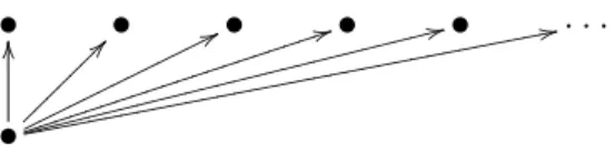
• • • • • . . . • OO ~?? ~ ~ ~ ~ ~ ~ 77o o o o o o o o o o o o o 44 i i i i i i i i i i i i i i i i i i i i 33 g g g g g g g g g g g g g g g g g g g g g g g g g g 22 e e e e e e e e e e e e e e e e e e e e e e e e e e e e e e e e e
Fig. 1. Tree for Example 1.
as a projective limit of finite sets. Therefore R is in particular closed in D. Since R ⊇ MD, this implies that R contains the closure of MD. Hence R = C.
✷
Theorem 3 Let D be a bifinite domain. Then the topological space MD of
maximal elements of D can be represented as a projective limit of finite sets if and only if MD is compact. In this case, MD is naturally represented as the
projective limit of the above projective system (Ri)i∈I.
Proof. It is clear that, if MD can be represented as a projective limit of finite
sets, then it is compact.
Conversely, assume that MD is compact. Then MDis closed in D, and therefore
MD coincides with its closure. It follows from Lemma 7 that the sub-projective
system (Ri)i∈I introduced above, which is a projective system of finite sets,
has its limit R that satisfies R = MD. ✷
The examples below show that compactness is not easy to guarantee. The two first examples show bifinite domains with non compact spaces of maximal ele-ments. Example 3 gives a sufficient condition for an event structure (see §2.5) to have a compact space of maximal configurations.
Example 1 A first simple example of bifinite domain D which space of max-imal elements is not compact is the following: take D to be the set of paths of the tree with one root, and countably many immediate successors (pictured in Figure 1). More formally, take I = N, the set of nonnegative integers, and Li = {0, 1, . . . , i} for i ∈ I, with the following ordering: 0 ≤ k for any k ∈ Li,
and otherwise the ordering is discrete. Then take, for i, j ∈ I with i ≤ j, gij : Lj → Li defined by gij(k) = k if k ≤ i and gij(k) = 0 otherwise. Then gij
is member of the projection-embedding pair with lower adjoint gbij : Li → Lj
defined by gbij(k) = k for k ∈ Li. The bifinite domain D, projective limit of
(Li)i∈I is given by L = N, with the discrete ordering on {1, 2, . . . }, and 0 as
bottom element. The space of maximal elements MD is given by {1, 2, . . . },
every element of which is a compact element of D. MD is thus an infinite set
of isolated elements, so it is not a compact space.
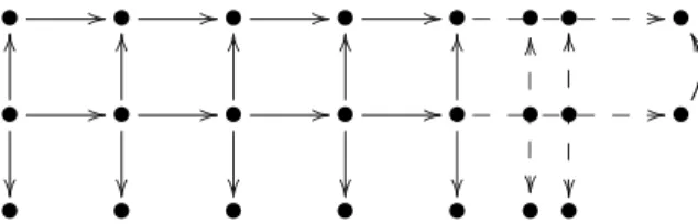
Example 2 In the above example, the bottom element 0 in D has infinitely many immediate successors. From a modeling viewpoint, we could prefer that finitely many actions should be enabled at any time. Unfortunately, this is not
• //• //• //• //•_ _•_•_ _ _//• • // OO ²² • // OO ²² • // OO ²² • // OO ²² •_ _ _ _ _ _// OO ²² • • ²² OOÂ Â Â Â Â OO ²² Â Â Â Â Â • XX • • • • • • •
Fig. 2. Bifinite domain for Example 2.
enough to guarantee compactness of the space of maximal elements. We leave to the reader to check that the poset pictured in Figure 2 is a bifinite domain (it can be seen as the domain of configurations of an event structure), with the property that every element has at most 3 immediate successors, but still with a non compact space of maximal elements.
Example 3 Let (E, ≤, #) be an event structure, and let D be the domain of configurations of E. Say that a downward closed subset P of E is intrinsic if, for every configuration ξ which is maximal in E, the set-theoretic intersection ξ∩ P , which is obviously a configuration of P , is maximal in P . Then we have: if every e ∈ E belongs to some finite intrinsic downward closed subset of E, then the space MD is compact. Indeed, we check in this case that the space
MD is closed in D, and thus compact.
5 Conclusion
We have presented a self-contained study of bifinite domains based on their representation as projective limits of projective systems of finite type. We have studied the relationship between the projective topology of bifinite domains and their usual topologies that come from Domain theory, showing that the projective topology coincides with the Lawson topology. As an application, we have established for bifinite domains the one-to-one correspondence between continuous valuations and Radon measures. Finally, motivated by probabilistic considerations, we have given a concrete representation of the space of maximal elements of a bifinite domain as a projective limit of finite sets if this space is compact—which is the necessary and sufficient condition for the existence of such a representation.
Future work goes along two lines. First, it would be interesting to extend the techniques of projective systems of measures used here in frameworks more general than bifinite domains. Secondly, the probabilistic interpretation can be pushed further. Domain, and in particular bifinite domains, present a suitable framework for partially ordered stochastic processes. In particular, we expect to successfully apply to domains the theory of martingales with partially ordered, directed sets.
References
[1] S. Abbes and A. Benveniste. Probabilistic models for true-concurrency: branching cells and distributed probabilities for event structures. Information and Computation, 204(2):231–274, 2006.
[2] M. Alvarez-Manilla, E. Edalat, and N. Saheb-Djahromi. An extension result for continuous valuations. Journal of London Mathematical Society, 61(2):629–640, 2000.
[3] A. Benvensite, S. Haar, and E Fabre. Markov nets: probabilistic models for distributed and concurrent systems. IEEE Transactions on Automatic Control, 48(11):1936–1950, 2003.
[4] P. Billingsley. Convergence of probability measures, second edition. John Wiley, 1999.
[5] N. Bourbaki. Int´egration, chapitre ix. ´El´ements de Math´ematiques, fascicule xxxv. Hermann, 1961.
[6] G. Gierz, K. Hofmann, K. Keimel, J. Lawson, M. Mislove, and D. Scott. Continuous Lattices and Domains. Cambridge University Press, 2003.
[7] C. Gunter. Profinite solutions for Recursive Domain Equations. PhD Thesis. University of Wisconsin, 1985.
[8] A. Horn and A. Tarski. Measures in boolean algebra. Transactions of American Mathematical Society, 64(3):467–497, 1948.
[9] P.T. Johnstone. Stone spaces. Cambridge University Press, 1982.
[10] A. Jung. Cartesian Closed Categories of Domains. CWI Tracts, volume 66. Centrum voor Wiskunde en Informatica, Amsterdam, 1989.
[11] A. Jung. Classification of continuous domains. Proceedings of the Fifth Annual IEEE Symposium on Logic in Computer Science, pages 35–40. IEEE Computer Society Press, 1990.
[12] K. Keimel and J.D. Lawson. Measure extension theorems on T0-spaces.
Topology and its Applications, 149:57–83, 2005.
[13] J. Lawson. Continuous Lattices and Related Topics, volume 27 of Mathematik Arbeitspapiere, chapter Valuations on continuous lattices, pages 204–225. Universit¨at Bremen, 1982.
[14] M. Nielsen, G. Plotkin, and G. Winskel. Petri nets, event structures and domains, part 1. Theoretical Computer Science, 13:85–108, 1981.
[15] G. Plotkin. A powerdomain construction. SIAM Journal on Computing, 5:452– 487, 1976.
[16] D. Varacca, H. V¨olzer, and G. Winskel. Probabilistic event structures and domains. In Proceeding of CONCUR 2004, International Conference on Concurrency theory, volume 3170 of LNCS, pages 481–496, 2004.