Borehole Stoneley Wave Propagation Across Heterogeneous And Permeable Structures

ACROSS HETEROGENEOUS AND PERMEABLE

STRUCTURES

by

X.M. Tang

New England Research, Inc. 76 Olcott Drive

White River Junction, VT 05001

and

C.H. Cheng

Earth Resources Laboratory

Department of Earth, Atmospheric, and Planetary Sciences Massachusetts Institute of Technology

Cambridge, MA 02139

ABSTRACT

This study investigates the propagation of borehole Stoneley waves across heterogeneous and permeable structures. By modeling the structure as a zone intersecting the borehole, a simple one-dimensional theory is formulated to treat the interaction of the Stoneley wave with the structure. This is possible because the Stoneley wave is a guided wave, with no geometric spreading as it propagates along the borehole. The interaction occurs because the zone and the surrounding formation possess different Stoneley wavenumbers. Given appropriate representations of the wavenumber, the theory can be applied to treat a variety of structures. Specifically, four types of such structures are studied, a fluid-filled fracture (horizontal or inclined), an elastic layer of different properties, a permeable porous layer, and a layer with permeable fractures. The application to the fluid-filled planar fracture shows that the present theory is fully consistent with the existing theory and accounts for the effect of the vertical extent of an inclined fracture. In the case of an elastic layer, the predicted multiple reflections show that the theory captures the wave phenomena of a layer structure. Of special interest are the cases of permeable porous zones and fracture zones. The results show that, while Stoneley reflection is generated, strong Stoneley wave attenuation is produced across a very permeable zone. This result is particularly important in explaining the observed strong Stoneley attenuation at major fractures, while it has been a difficulty to explain the attenuation in terms of the

8 Tang and Cheng

(

planar fracture theory. In addition, by using a simple and sufficiently accurate theory to model the effects of the permeable zone, a fast and efficient method is developed to characterize the fluid transport properties of a permeable fracture zone. Tills method may be used to provide a useful tool in fracture detection and characterization.

INTRODUCTION

Fractures or permeable structures in reservoirs are of great importance in the exploration and production of hydrocarbons. Heterogeneous layers in the formation are also of ma-jor significance. A very good example of such heterogeneous and permeable structures is the sand-shale sequence found in sedimentary formations. Full waveform acoustic log-ging offers an effective tool for characterizing these structures. The current technique for modeling borehole acoustic wave propagation with heterogeneous formation structures is finite difference method (Bhashvanija, 1983; Stephen et aI., 1985; Kostek, personal communication). Tills technique can handle heterogeneity quite easily. However, the im-plementation of the method to a permeable porous formation is still a topic of research. Although wavenumber integration technique can be used to calculate wave propagation in homogeneous porous formations (Rosenbaum, 1974; Sclunitt et aI., 1988), it is very difficult, ifnot impossible, to apply such a technique to treat problems involving porous layer structures. In tills study, we will show that if only the low-frequency Stoneley wave is used, the interaction of acoustic waves with borehole permeable structures can be much simplified. The objective of this study is to develop a theoretical model ,that can be used to calculate borehole Stoneley wave propagation across heterogeneous and permeable structures. As a result, the properties of such structures can be characterized by means of Stoneley wave measurements.

The Stoneley (or tube) wave has been used as a means of formation evaluation and fracture detection. This wave mode dominates the low-frequency portion of the full waveform acoustic log due to its relatively slow velocity and large amplitude. Because this wave is an interface wave borne in borehole fluid, the Stoneley is sensitive to such formation properties as density, moduli, and most importantly, permeability or fluid transmissivity. It is expected that any change of these properties due to a formation heterogeneity will result in the change of Stoneley propagation characteristics, allow-ing the heterogeneity to be characterized usallow-ing Stoneley wave measurements. Borehole fractures are an example of such heterogeneity. Paillet and White (1982) observed that attenuation of the Stoneley wave occurs in the vicinity of permeable fractures. Hornby et al. (1989) showed that permeable fractures also give rise to reflected Stoneley waves. Theoretical studies using finite difference (Stephen et al. 1985; Kostek, personal com-munication) and other techniques (Hornby et aI., 1989; Tang, 1990) have been carried out to model the effects of a borehole fracture. In all these models, the analogy of a parallel planar fluid layer was commonly adopted to represent the fracture. Laboratory

model experiments that comply with this analogy have yielded results that agree with the theoretical results (Tang and Cheng, 1988; Hornby et aI., 1989). Although both at-tenuation and reflection of the Stoneley wave are predicted by the plane-fracture model, it takes a rather large fracture aperture (on the order of a centimeter) to attenuate the Stoneley wave significantly. However, fractures with such apertures are rarely found in the field (Hornby et aI., 1989), but Stoneley wave attenuation (up to 50% or more) across in situfractures is co=only observed (Paillet, 1980; Hardin et al., 1987). Until now, there has not been an effective model to account for the significant Stoneley wave attenuation observed in the field. Paillet et al. (1989) suggested that in situ fractures may consist of an array of flow passages or fracture layers, instead of a single fluid layer. In this study, we substantiate this hypothesis by modeling fractures as a permeable zone in the formation. Key parameters that are used to characterize the permeable zone are thickness of the zone, permeability, fracture porosity, and tortuosity. Since the last three parameters are typical parameters of a porous medium, we can use the Biot-Rosenbaum theory (Rosenbaum, 1974) to model the Stoneley wave characteristics in the permeable zone. Tang et al. (1990) have recently developed a simple model for Stoneley propagation in permeable formations. This model yields results consistent with the analysis of Biot-Rosenbaum theory in the presence of a hard formation, but the formulation and calculation are much simplified. The use of this simple theory in modeling the permeable zone will allow the development of a fast and efficient algorithm to characterize the effects of the zone on Stoneley waves.

In the following, we first develop a theory for the Stoneley wave interaction with a borehole structure. Then we will apply it to the planar fracture case in connection with the existing theory. The case of an elastic layer will also be studied because of its relevance to the wave phenomena of a layered structure. Finally and most importantly, we study the cases of a permeable zone and a fracture zone and present some theoretical results.

THEORETICAL FORMULATION

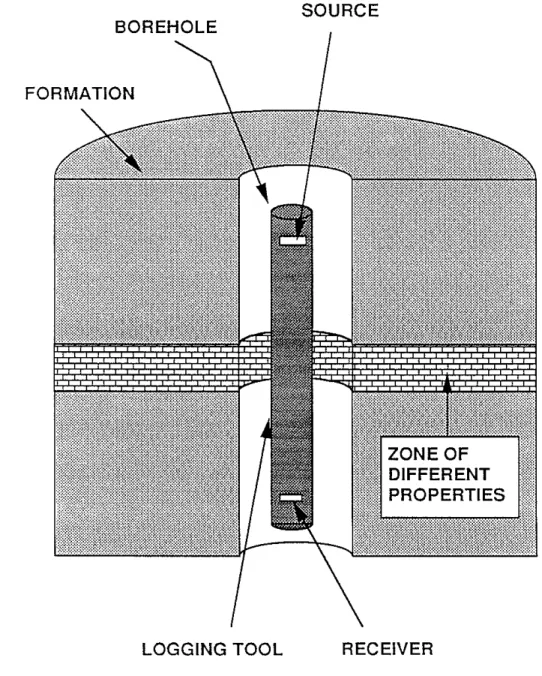
We consider a zone of different properties sandwiched between two formations of the same properties. The upper and lower boundaries of the zone are located at z = 0 and z = L (L is thickness of the zone) along the borehole axis, respectively. A

fluid-filled borehole of radius R penetrates the zone and the formations. The logging tool is simulated as a rigid cylinder of radius a at the borehole center. Figure 1 illustrates the configuration. We assume that the logging is performed at frequencies below the cut-off frequency of any mode other than the fundamental (Stoneley), so that the borehole fluid pressure may be considered as approximately uniform across the fluid annulus between the tool and the borehole wall. In other words, the problem is now approximated as a one-dimensional wave propagation problem. In the formations above and below the

10 Tang and Cheng

(

zone, the wave equation for the Stoneley wave is

d27/J

- - 2

+

kr7/J

=

0 ,

z

<

0,

z

>

L

dz (1)

where

7/J

is the Stoneley wave displacement potential and

k

1 is the axial Stoneley wave number in the two formations of the same properties. In the region where the zone is located, the wave equation is

(2)

where k₂ is the axial Stoneley wave number of the zone. In terms of the potential

7/J,

the fluid pressure P and axial displacement of the Stoneley wave are given by

(

(3)

(4)

where Pf is fluid density andw is the angular frequency. The coupling of wave motions at the boundaries z = 0 and z = L is now considered. Although there are some radiation effects at the interfaces outside the borehole in the formation (White, 1983), the Stoneley wave energy is mostly contained in the borehole, so that the effects due to the coupling outside the borehole are small compared to those due to the coupling in the borehole. Therefore, we only consider the fluid coupling in the borehole. The coupling (or interaction) arises because of the difference between the propagation constants k1 and k2, due to the fact that the properties of the zone are different from those of the

formations. Thus the boundary conditions for the coupling can be specified. That is, at the z

=

0 and z

=

L, the fluid displacement and pressure must be continuous.

The solutions to Eqs. (1) and (2) can now be given. Let us consider a Stoneley wave

A(w)eik1z _{incident from thez}

_<

_{0 region onto the heterogeneous zone. Upon interacting} with the zone, part of the energy will be reflected back from the zone. Thus in thez

<

0 region, there are both incident and reflected waves, giving a solution in the form of

(

(

(

(5) where A'e-ik1Z _{represents the reflected wave propagating in the negative-z direction} and A' is the reflected amplitude coefficient. In the 0

<

z

<

L region where the zone is

located, there are waves propagating in both positive- and negative-z directions, these waves being generated by the transmission and reflection occurring at the z

=

0 and

z

=

L boundaries. The solution is written as

where B and B' are respectively the amplitude coefficients for waves propagating in the positive- and negative-z directions. In the z

>

L region, there are only waves transmitted from the zone, and the solution is given by

(7) whereC is the amplitude coefficient of the transmitted waves. The coefficients are to be determined from the conditions that the fluid pressure and displacement be continuous across thez

=

0 andz

=

L boundaries. From Eqs. (3) and (4), it can be seen that these conditions are expressed as the continuity of"if;and

~~

across the boundaries. By using the solutions given in Eqs. (5), (6), and (7) and the continuity conditions, the following simultaneous equations are obtained.

A+A' = B+B'

,

(8)

k1(A- A') k2(B - B') (9)

Beik2L

+

B'e- ik2L

₌

CeiklL

,

(10)

k2(B eik2L - B'e-ik2L) klCeiklL ₍₁₁₎

In terms of the incident amplitude coefficient A, the coefficients A', B, B', and C are determined as

A'IA BIA B'IA CIA

= 2i(k~ - ki) sin(k2L)1D ,

= _2k1(k1

+

k2)e-ik2L I D , = 2k1(k2 - kdeik2LID 4klk2e-ik2L ID (12) (13) (14) (15)

where the denominator D(w) is given by

D

=

_{(k 1}

+

_{k2)2e-ik2L - (k1 _ k2)2eik2L (16)}

The incident amplitude Ais related to the source excitation of the Stoneley wave mode.

Ifthe source is located at distance h from z = 0, then A can be written as

A(w) = S(w)E(w)eik1h , (17) where Sew) is the source spectrum as a function of frequency and E(w) is the Stoneley wave excitation function that is dependent on the borehole and tool radii and formation and fluid properties. A formulation ofE(w) is given by Tang and Cheng (1991). For the purpose of modeling synthetic seismograms, a Kelly source (Kelly et aI., 1976) can be used for the source spectrumSew). Given a center frequencyWQ of the sourceSew), one can choose the maximum frequencyWmax as 2.5wQ, at which Sew) is vanishingly small. The coefficients A', B, B', and Care then evaluated for each increasing frequency up to

12 Tang and Cheng

(7), and then Eq. (3) to calculate the fluid pressure in the different regions as a function of frequency. The results are then transformed into the time domain by using the fast Fourier transform. In this manner, synthetic seismograms at each given z in the region

of interest can be obtained, which display the wave characteristics in the vicinity of the heterogeneous zone.

APPLICATIONS

We have given a simple formulation for calculating Stoneley wave propagation across a borehole structure. This formulation is quite general because it can be used to treat a variety of borehole structures. In the above formulation, we placed no restriction on the nature of the borehole structure. In fact, this structure can be a fluid-filled fracture (horizontal or inclined) capable of conducting fluid away from the borehole. This structure can also be an elastic layer sandwiched between two elastic formations whose elastic constants are different from those of the layer. Furthermore, the structure can be a permeable porous zone between two impermeable formations. Most important, when appropriate parameters are used for the porous medium, this zone can be used to model the effects of a permeable fracture zone intersecting the borehole. The properties of the heterogeneous zone are characterized by the propagation constant k2. As we will see in the following, given appropriate representations ofk2 , the above formulation can be used to model the effects of a fluid-filled fracture, an elastic layer, a porous zone, and a permeable fracture zone.

Fluid-filled Fracture

The case of a fluid-filled fracture intersecting the borehole is of particular interest be-cause, with existing theory for this case, it offers a direct test of the validity and ver-satility of the present formulation. Assuming that the formation is rigid, Tang and Cheng (1988) as well as Hornby et al. (1989) have formulated a theory for calculating the transmission and reflection of Stoneley waves at the fracture. Hornby et al. (1989) even considered the case of an inclined fracture. Although the assumption of a rigid formation may seem too restrictive, later theoretical studies with an elastic formation (Tang, 1990; Kostek, personal communication) only slightly modify the rigid formation results. We will use the rigid formation theory to test our present theory. The key point in utilizing the present theory is to find the wavenumber k2 that characterizes the structure, I.e., the fluid-filled fracture. We first study the case of a horizontal fracture. Then we will extend the formulation to treat the case of an inclined fracture.

(

Horizontal Fracture

- J

if.dS=~

r

-PdV (18)

J

s

Pjvj

J6.V '

where ifis the fluid particle velocity, (i.e., if

=

-iwU), /':,.V

=

1rR2L is the volume of

the borehole section located at the fracture opening, and Sis the surface enclosing /':,.V.

The normal to S is pointed outwards from /':,.V. With the aid of Figure 2a, we calculate the surface integral of the fluid flux in Eq. (18). At z

=

0, the axial fiux is iwU(0)1rR2 At z = L, it is -iwU(L)1rR2, where U is the axial fluid displacement. In the radial direction, the flux per unit fracture length is given by (Tang and Cheng, 1988)

-dP

q

=

-Cdr ' (19)

where

C

=

iL/wPf is the fracture dynamic conductivity without viscous effects (the effect of viscosity is neglected here), and

~~

is the radial pressure gradient at the fracture opening, which, according to Tang and Cheng (1988), is given by

dP

=

-Pk

oH;l) (koR) (20)

dr H2)(koR)

where P is now the pressure in the borehole section 0

<

z

<

L, and H~l) and H?) are Hankel functions of order zero and one. For rigid fracture surfaces, the fracture wavenumber is ko = w/Vf, i.e., the free space wavenumber, where _Vf is acoustic velocity of the fiuid. The radial flux is 21rRq. The volume integral of Eq. (18) is simply P/':,.V. With these quantities specified, Eq. (18) may now be written as

[U(L) - U(0)]1rR2

+

21rRq

=

iWV2P1rR2 L (21) Pf f

Dividing Eq. (21) by1rR2L and usingU

=

A

ddP (Eqs. 3and4) and the approxima-Pfw z

tion

Consider a horizontal fracture intersecting the borehole (Figure 2a). For comparison with the existing fracture theory of propagation in a fluid-filled borehole, the effects of the logging tool are dropped. The fracture has a thickness L and is bounded by a rigid formation. In order to find k₂ in the 0

<

z

<

L region where the fracture is located, we use the equation of mass conservation for a small amplitude wave (Tang and Cheng, 1988)

U(L) - U(O) dU

L "" dz '

we obtain a wave equation for the borehole pressure P in the 0

<

Z

<

L region, given as

d2P

[2

2ko H;l)(koR)]

- d2

+

k

o -

R (1) P

=

0 , 0

<

z

<

L .

z _{H o (koR)}

14 Tang and Cheng

(

This means that the wave motion in this region is characterized by a wavenumber

1 _ 2 Hil)(ka R)

koRHal)(koR) (23)

The wavenumber in the z

<

0 and z

>

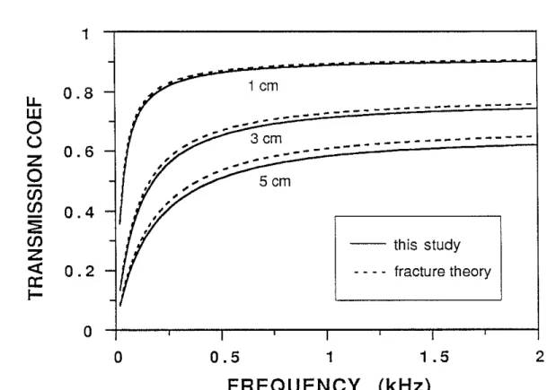
L regions is simply kl = w/Vf because of the rigid formation (White, 1983). With known kl and k2 ,we can now calculate the effects of a horizontal fracture on Stoneley propagation using the present theory. Figure 3 shows the amplitude of Stoneley wave transmission coefficient versus frequency (solid curves) for three different fracture thicknesses, L = 1 cm, 3 cm, and 5 cm, calculated using Eq. (15). The borehole radius is R=lO cm and fluid velocity is Vf =1.5 km/s. The theoretical results from Hornby et al.'s (1989) fracture theory are also calculated and plotted in the same figure (dashed curves). To our satisfaction, the two theories are in very good agreement. For the 1 cm fracture case, the agreement is excellent. This agreement validates our present theory. Furthermore, the two theories show some differences as the fracture thickness increases, the present theory showing slightly lower values than the Hornby et al. theory for the L

=

3 cm and 5 cm cases. This difference arises because the effect of the vertical extent of the fracture is not negligible when L

is big. Under the same assumption of homogeneous flow across the fracture opening, Hornby et al.'s (1989) theory neglects the vertical extent of the fracture (since in situ fractures of several centimeter thick are rare), while the present theory accounts for this effect. The effect of the vertical extent may become pronounced in the case of an inclined fracture, which will be studied in the next section.

Inclined Fracture

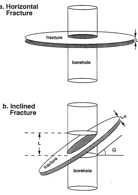
The configuration of an inclined fracture is illustrated in Figure 2b. The fracture crosses the borehole at an angle Bmeasured from the horizontal plane. We now use La to de-note the thickness of the fracture and L the vertical extent of the fracture within the borehole, as indicated in Figure 2b. Within the plane of the fracture, the borehole makes an elliptical hole, which is also indicated by the shaded area in the figure. The semi-minor axis of the ellipse is the borehole radius R, whereas the semimajor axis is

R

L

_o

RI = - -

+

-tanB

cosB 2

In comparison with the horizontal fracture case, the present case will have two additional effects on the Stoneley propagation. In the first, the flow into the fracture opening is modified due to the elliptically-shaped borehole-fracture boundary. The second is that the vertical extentLmay become comparable to the wavelength asBincreases, which will modify the wave motion within the 0

<

z

<

L region. We address the first effect first, and then incorporate it and the second effect into our theory to give the final results. The first effect has been studied by Hombyet al. (1989). In order to solve for the flow into the elliptical boundary, they transformed the problem to elliptic coordinates and

found the solution as a series summation of Mathieu functions. Because of this, the analysis and the solution are quite involved. In the this study, we take a very simple alternative approach. We simply replace the ellipse with an equivalent circle that has the same perimeter as that of the ellipse. Therefore, the radius of the circle

R

is given by the equation

211"R

=

perimeter of ellipse

=

4RIE(e,

~)

, (24)

where E(e,11"/2) is a complete elliptic integral of the second kind, ande

=

J

R~

- R2/ R1 is eccentricity of the ellipse. The flow per unit fracture length is given by Eq. (19), which shows that the flow is driven by a pressure gradient. For the elliptical boundary, the pressure gradient is the largest in the semi-minor axial direction and the smallest in the semi-major axial direction. For the equivalent circle whose radius lies between Rand

R1 (R

<

R

<

Rd,

the pressure gradient -PkoHil\koR)/Hal)(koR) (Eq. 20) should also lie between the two extremes. Therefore, the total flow along the ellipse perimeter is expected to be approximately the same as the total flow along the equivalent circle perimeter, which is given by211"Rq. In terms ofk2 , this is equivalent to changing Eq. (23) to

k

2

=.!:!...

1 _

2R

Hi

l

)(koR)

Vf koR2 Hal) (koR)

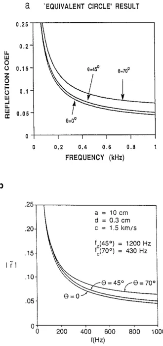
The modified k2 can then be used to calculate the transmission and reflection of the Stoneley wave at the fracture. The results can be compared with those of Hornby et al. (1989) obtained using Mathieu functions. At this stage, the zone thickness in Eq. (12) is still treated as the fracture thickness £0, since the effect of vertical extent is not accounted for in Hornby et al.'s theory. Figure 4a shows the amplitude of the reflection coefficient (Eq. 12) in the frequency range of [0,1] kHz. The results are calculated for

o

= 0°, 45°, and 70°. The thickness of the fracture is 0.3 cm and the borehole radius

and fluid velocity are the same as before. The original results of Hornby et al. (1989) calculated for the same parameters are given in Figure 4b. The agreement between the two sets of results is very good. For the 0

=

0° case, the results in the two separate

figures are in almost exact agreement. Using this case as the basis, we can compare the

o

=45° and 70° curves in the separate figures. The results of our simple approach are

very close to the results of Hornby et al.'s approach, except that our 0=70° curve has

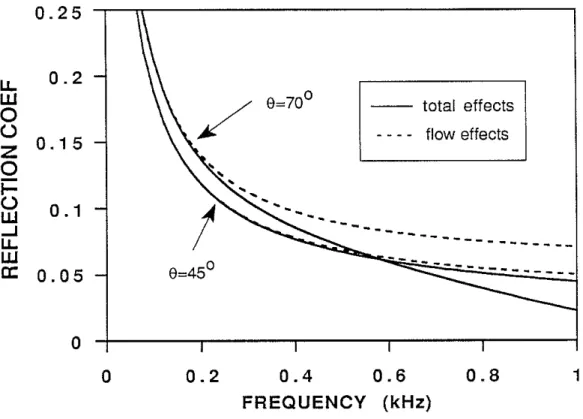
slightly higher values than Hornby et al.'s result. This comparison shows that the flow effect due to the inclined fracture is adequately accounted for by using the equivalent circle in our theory. However, as pointed out by Hornbyet al. (1989), the results shown on Figures 4 will become invalid when the wavelength is comparable to the vertical extent of the fracture. This effect will be addressed in the following.

The vertical extent of the fracture within the borehole (Figure 2b) is obviously given by

£0 £ = 2RtanO

+

--0

16 Tang and Cheng

(26) We now need to find an equivalent wavenumber k2 that charaderizes the overall wave motion in the 0

<

z

<

£ region. To do this, we simply repeat the derivation for the horizontal fracture case (Eqs. 18 through 23), in which we account for the flow into the elliptical fracture opening by replacing the borehole radius R in the flow term 271'Rq in

Eq. (21) with the equivalent circle radius

R

given by Eq. (24). The final expression for the wavenumber is

k2

=.!'!...

1 _ £0

2R

HP\koR) VI £ koR2 Hal) (koR)

Using this k2 and the zone thickness £ (Eq. 25), we recalculate the curves of Figure 4a for the

e

= 45° and 75° cases. The results are shown in Figure 5 (solid curves). For

comparison, the curves of Figure 4a are replotted (dashed curves). For

e

= 45°, the

vertical extent £ is about 20 em. For

e

= 70°, it is 56 em. The frequencies at which the

wavelength is comparable to £ (i.e., k

_o

£ '" 1) are 1.2 kHz and 0.43 kHz, as indicated

in Figure 4b. As shown in Figure 5, below these frequencies the effect of vertical extent is lninimal, as expected. The solid and dashed curves approach each other towards low frequencies. However, above the frequencies, this effect significantly reduces the refiection coefficient (see the

e

= 70° case). This indicates that high angle fractures act

more like an attenuator than a reflector at higher frequencies.

The application of the present theory to the planar fracture case demonstrates that the theory not only is fully consistent with the existing fracture theory, but also accounts for the effect of vertical extent in the presence of a high angle fracture. Thus it presents a simple method that can be applied to cases where the planar fracture analogy is applicable.

Elastic Layer

We now consider the case of an elastic layer sandwiched between two elastic formations. For an elastic formation, the wave numberkof the Stoneley wave in a fluid-filled borehole containing a rigid tool at bore center is deterlnined by the following borehole period equation (Tang and Cheng, 1991, Schlnitt, 1988)

where In and K n (n=O,I) are the first and second kind modified Bessel functions, p is formation density, c = w/kis the Stoneley wave phase velocity. The radial wavenumbers

are I, m, and j, given by

where Vp and Vs are formation compressional and shear velocities, respectively. For given respective elastic velocities and density of the layer and of the surrounding for-mations, the wavenumbers k2 and k1 can be respectively determined as a function of frequency from the period equation (Eq. 27). With k1 andk2 known, Eqs. (12) through (16) are used to calculate the Stoneley wave propagation across the elastic layer.

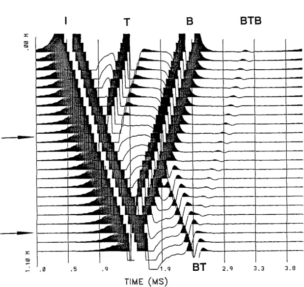
Figure 6 shows the synthetic array waveforms for the Stoneley propagation across an elastic layer of 50 cm thick. The parameters used in the calculation are: Pl =2.4

kg/m3 , Vp1=4 km/s, and Vsl=2.3 km/s for the formation and P2=2.1 g/cm3, Vp2=2.4 km/s, and _{Vs2=1.4 km/s for the layer. The borehole fluid density and velocity are}

Pf =1 kg/m3 _{and Vf=1.5 km/s. The bore and tool radii are R=10 cm and a=4 cm,}

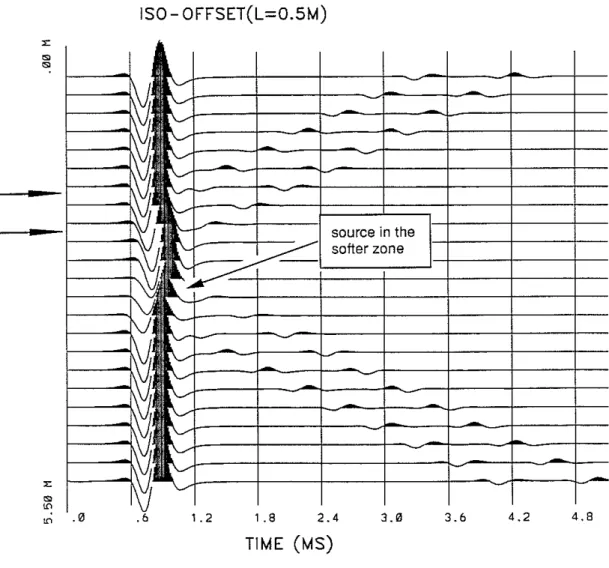
respectively. The source center frequency is 5 kHz. In this figure, wave amplitudes are largely enhanced and large amplitudes are clipped to show small amplitude reflected events. An interesting feature of this figure is that multiple reflections are generated at the top and bottom interfaces of the layer. As shown in Figure 6, an incident Stoneley wave (I) is excited at about 1 m above the layer. Upon impinging on the top interface, a reflection (T) is generated. At the bottom interface, a reflection (B) is also generated. When the bottom reflection (B) crosses the top interface, a secondary reflection (BT) is generated which propagates across the bottom interface, generating again another reflection (BTB) of very small amplitude. The predicted multiple reflection events show that our simple formulation correctly captures the wave phenomena of a layered structure. In logging measurements, waves are often received by fixing the source-receiver distance and moving the tool along the borehole. This is called the iso-offset measurement. Figure 7 shows the calculated iso-offset seismograms across the layer. The source center frequency now is 3 kHz. The source-receiver spacing is 1 m. Other parameters are the same as those in Figure 6. In addition to the two primary reflected events (T and B of Figure 6), the waves transmitted across the layer also show some interesting features. First, the Stoneley wave is delayed when the layer is between the source and the receiver, because of the relatively slower Stoneley velocity in the layer (the velocity is about 1.2 km/s in the layer and 1.4 km/s outside). Second, below the layer, the transmitted waves show a reduction in amplitude, as indicated in the figure. This is due to the fact that when the source is passing through the layer that is softer than the surrounding formation, the excitation of the Stoneley wave is lower than when the source is in the surrounding formation (see Tang and Cheng, 1991). Since borehole fractures also result in the reduction of Stoneley wave amplitude (Paillet, 1980), one must be careful in order not to mistake this excitation effect for the effects of fractures when interpreting an acoustic log. When both source and receiver are below the layer, the up-going waves emitted from the source are also reflected by the two interfaces, as can be seen from the two down-going reflections in Figure 7.

18 Tang and Cheng

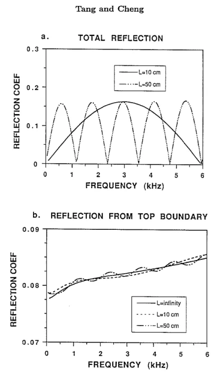
Although multiple reflections are generated at the two interfaces, the two primary reflections (T and B of Figure 6) are of major importance, the amplitude of the secondary and other reflections being negligibly small. This can be seen from the amplitude ratio At/A (Eq. 12) which governs the total reflected wave energy (we call At /A the

total reflection coefficient of the layer). Figure 8a plots the amplitude of At/ A versus

frequency for two different layer thicknesses. They are L=50 em and L=10 em. The

formation and layer properties are the same as before. The total reflection coefficient shows mainly the superposition of the two primary reflected waves (T and B), the two waves being almost equal in amplitude with the bottom reflection (B) having a phase lag of 2k2L. Because of the superposition, the total reflection At/ A shows a periodic

spectrum that contains a number of maxima and minima (zeros). The period of the maxima or minima is approximately

(

(

6.f

= Vst

. 2L ' (28)

(29) where Vst is the average Stoneley velocity within one period. This relation can be easily obtained using Eq. (12). The implication of Eq. (28) to field measurements is that, if the periodicity can be determined from the reflected Stoneley wave spectrum, Eq. (28) may be used to deduce the thickness of the layer structure. For example, taking V_St =1.2

km/s as calculated for the given layer parameters and using the

6.f

measured from Figure 8a for the two curves of different thicknesses, we obtain L :::;50 em and 10 em, respectively, in agreement with the true values.

In the case of a very thick zone where the top and bottom reflections are far apart and can be measured individually, the reflection coefficient for waves reflected from the top interface can be derived from Eq. (12) by noting that

2isin(k2L) = eik2L _ e-ik2L .

The reflection coefficient is

(k 2 _ k2)e-ik2L

RC= 1 2 .

(k 1

+

k2)2e-·k2L - (k1 - k2)2e·k2L

Using the same parameters as above, we have calculated Eq. (29) for three different L

values, L=10 em, L=50 em, and L

=

00. The results are shown in Figure 8b. The RC curves for L=50 em and L=10 em fluctuate slightly around the single boundary case

(L

=

00). In practice, the small deviations are hardly measurable and the three curves in Figure 8b can be treated as the same. This means that, regardless of the thickness

of the layer, the reflection from the top interface is almost equivalent to the reflection from the interface between two semi-infinite formations. In fact, when L -> 00,we have

eik,L -> 0 and e- ik2L -> 00 (if we assume that k2 contains a small positive imaginary part). Eq. (29) reduces identically to

RC _ k1 - k2

- k₁

+

k₂ '

in agreement with White (1983).

A case of particular interest in acoustic logging is the effect of a very thin elastic layer on the reflection of Stoneley waves. To illustrate this effect, we have calculated the iso-offset seismograms of Figure 9. The parameters are the same as those used in Figure 7, except that the layer thickness is now £ =10 cm. Because of the thin layer (indicated by arrows), the top and bottom reflections overlap in the time domain and interfere constructively to give a single reflected wave whose amplitude is nearly doubled compared with each individual reflection in Figure 7. This can also be seen from the total reflection curve in Figure 8a (the £=10 cm curve), where the the value of the total reflection around 3 kHz is nearly twice the top reflection coefficient of Figure 8b. This example shows that a very thin elastic layer (hard or soft) may result in a strong reflection due to the constructive interference of the top and bottom reflections.

Permeable Porous Layer

The case of a porous layer sandwiched between two elastic formations will be studied here. This situation is of special interest in acoustic logging through layered reservoirs where a permeable porous layer is sandwiched between two impermeable formations. The porous layer can be modeled as a Biot solid (Biot, 1956a,b). The problem of wave propagation in permeable boreholes was first treated by Rosenbaum (1974). The model is referred to as the Biot-Rosenbaum model (Cheng et aI., 1987). Using the theory of dynamic permeability (Johnson et

aI.,

1987), Tang et al. (1990) have obtained a much simplified version of the Biot-Rosenbaum model. The simple model gives consistent results with the complete theory of the Biot-Rosenbaum model in the presence of a hard formation. In a soft formation, the two models agree in the low frequency range (up to about 2 kHz). The effect of a rigid logging tool can also be incorporated into the simplified model (Tang and Cheng, 1991). Using the simple model of Tang et al. (1991) for the porous layer, the wavenumber k2 in the 0

<

z

<

£ zone is given by a simple, explicit expression.

(30)

with

where Kf, Po, and J.L are pore fluid bulk modulus, density, and viscosity, respectively, ¢ is porosity, and t; is a correction for elasticity of the solid matrix (see Tang et aI., 1990). The symbol ketl is an 'equivalent elastic' Stoneley wavenumber with a rigid tool in the borehole. Itis calculated using Eq. (27) with the effective density and moduli (or

20

Tang and Cheng

(

velocities) of the fluid-saturated porous solid. If the density and velocities are given for the dry rock, they can be converted to the fluid-saturated properties using Gasmann's equation (White, 1983). A critical parameter in Eq. (30) is the dynamic permeability given as (Johnson et al., 1987)

(31) (

where 1<0 is the static Darcy permeability, a is the high-frequency limit of the dynamic tortuosity, which is a parameter describing the tortuous, winding pore space. The symbol A is a measure of pore size and is approximately given as (Johnson et al., 1987)

II.~ C~I<O)

(32)

In the case of fractures, A is the fracture aperture and the number 8 in Eq. (32) is replaced by 12. The dynamic permeability captures the frequency-dependence of fluid flow in porous media and makes the simple theory (Eq. 30) consistent with the Biot-Rosenbaum theory even at high frequencies. Using Eq. (30), we can calculate the Stoneley wavenumber k2 in the porous zone much more efficiently than using the Biot-Rosenbaum theory.

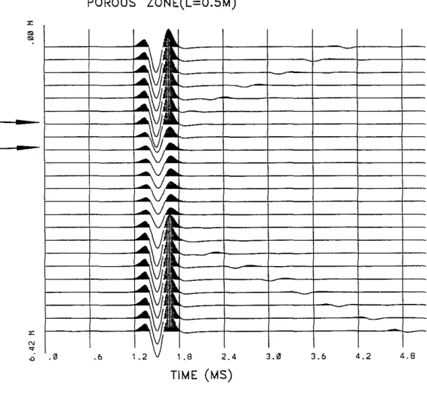
To illustrate the effects of a porous zone on the Stoneley propagation, we have calculated the synthetic iso-offset seismograms across a zone 50 cm thick. The source center frequency is 3 kHz and the source-receiver spacing is 2 m. We assume that the porous zone is saturated with the borehole fluid with Po = Pf =1 kgjm3 and Vf =1.5 kmjs. The formation and porous matrix properties are the same as in the previous elastic formation case. For the porous zone, we assume 1<0=5 Darcies, if> =30%, and

a=3. Figure 10 shows the synthetic waveforms. The location of the zone is indicated on

the figure (arrows). It can be seen that when the zone is between the source and receiver, the transmitted waves across the porous zone show significant amplitude attenuation, because of the loss of Stoneley wave energy into the porous zone. In addition, some weak reflections are generated. The waves reflected from the top and bottom interfaces no longer have the comparable amplitudes as in the elastic layer case. This comes from the fact that the wavenumber k2, as given in Eq. (30), contains an imaginary part that characterizes the attenuation of the waves iIi the zone. As a result, when the attenuated wave is reflected by the bottom interface, the generated reflection is already smaller than the top reflection. Furthermore, the smaller bottom reflection is further attenuated when it propagates through the zone. Therefore, the reflected waves are mainly the reflection from the top interface. Figure 11 shows the transmission and reflection of the Stoneley wave at the porous zone. The transmission coefficient is simply defined as the amplitude ratio of the transmitted wave over the incident wave, i.e., C /A

given in Eq. (15). The Cj A curve shown in Figure 11 is only about 0.45 beyond 2

(

kHz. This accounts for the significant amplitude reduction of Stoneley waves shown in Figure 10. For the reflection coefficient, we plot both the total reflection (Eq. 12) and the top reflection (Eq. 29) curves. As seen from Figure 11, the total reflection (dashed) curve fluctuates around the top reflection (solid) curve. This means that the total reflection curve consists malnly of the top reflection, with the superimposition from the (weak) bottom reflection. Additionally, the total reflection also exhibits a number of maxima or minima. The frequency interval between two adjacent maxima or minima is approximately given by Eq. (28). If this frequency interval can be determined from the reflected Stoneley wave spectrum, it may also be used to infer the thickness of the porous zone. For example, /::".f measured from Figure 11 is about 1.3 kHz. The Stoneley velocity in the porous zone is about 1.3 km/s for the given parameters. Using these two numbers in Eq. (28) gives L "'50 em, agreeing with the true value. There is also another way to measure the thickness of the porous zone. As can be seen from seismograms of Figure 10, the zone in which Stoneley waves are significantly attenuated has a width that is approximately the sum of the source-receiver spaCing with the zone thickness. Knowing the source-receiver spacing, we can determine the zone thickness from the width of the zone with attenuated Stoneley waves.

The porous zone model presented here predicts that Stoneley waves can be signifi-cantly attenuated by a permeable porous layer intersecting the borehole. This model, with a slight modification, can be used to model Stoneley propagation across permeable fracture zones, which will be studied in the following.

Permeable Fracture Zone

Recent fracture characterization using electrical borehole scan reveals that many frac-tures mapped by a borehole televiewer consist of a large number of microfracfrac-tures (Hornby et al., 1990). This suggests that a fracture zone model, instead of the planar fracture model, is a better analogy for such in situ fractures. Let us consider how we can characterize the fracture zone using our formulation for a porous zone. Suppose that the zone of thickness L contains n small fractures with average width La. The fracture porosity ¢ is simply

¢ =nLo L

The average permeability KO of the zone is

KO =

nL5/12

= ¢

L5

L 12

This relation allows us to give an order-of-magnitude estimate of the fracture perme-ability KO from measured fracture width. Fracture width from electrical borehole scan measurements often ranges from 0.001 to 1 mID (Hornby et al., 1990.) For L

_o

=100 micron (p.m) and fracture porosity ¢ = 0.1, the estimated permeability is on the order

22 Tang and Cheng

{

of 100 Darcies. This indicates that a fracture zone may be characterized as a highly permeable zone. On the other hand, the concept of dynamic permeability can still be applied to flow in fractures. Tang et al. (1990) have shown that the dynamic perme-ability of a porous medium reduces almost identically to the dynamic conductivity of a single fracture when appropriate parameters for the fracture are used. For multiple fractures, the </J in Eq. (31) is now the fracture porosity and "0 is the average fracture permeability. Therefore, while we still use </J and"0to characterize the fracture zone, we

may anticipate that "0 may assume very high values. In addition, in using the dynamic

permeability in Eq. (31), we replace the number 8 in Eq. (32) by 12 in order to comply wi th the fracture geometry. Furthermore, an important parameter that should also be considered is a, the tortuosity of the flow channel. For a porous medium, a usually varies around 2 and 3. (Rosenbaum (1974) used a value of 3 in his paper). For a frac-ture, a is 1 since flow takes place along a straight channel (Tang et al., 1990). Infact, a is relatively insignificant in the low-frequency range where fluid-flow is characterized by viscous diffusion. However, for the very high permeability values considered here, a becomes an important factor controlling the dynamic fluid flow. As seen from Eq. (31), for very high

"0,

,,(w) ->iJ-L</Jj(apow). This means that at high frequencies, flow is more effectively conducted into a fracture zone (a=l) than into a porous zone (a=3). In order to illustrate this, we have recalculated the transmission coefficient of Figure 12 by replacing a

=

3 with a

=

1 and keeping other parameters unchanged. The result with

a=l is plotted against that with a

=

3 in Figure 11. As expected, the two results are nearly the same at low frequencies; but the former result becomes significantly lower than the latter result at high frequencies, meaning that more Stoneley wave energy is carried away into a fracture zone than into a porous zone.

We now give an example of modeling Stoneley wave propagation across a fracture zone. The zone thickness is assumed to be 40 cm. Suppose that the zone is intensely fractured. We use a fairly high porosity value </J=40%. Permeability "0is taken to be 20

Darcies; ais 1. Other parameters used for the porous zone modeling are kept unchanged. Figure 13 shows the synthetic iso-offset seismograms. The Stoneley wave is greatly attenuated across the fracture zone. The strong Stoneley wave attenuation modeled here is quite consistent with field measurements that Stoneley waves often 'disappear' in the vicinity of fracture zones (Hardin et al., 1987). In addition, the reflected Stoneley waves appear to be stronger than in the porous case shown in Figure 10. This is due to the fact that in the presence of the highly permeable zone, the Stoneley wavenumber given by Eq. (30) is a highly complex number which is significantly different from the Stoneley wavenumber k1 of the surrounding formation. The larger difference between k1 and k2 will produce a stronger reflection than the porous zone case. The predicted Stoneley wave reflection is also consistent with the field observation of Hornby et al. (1989), which shows that permeable fractures also give rise to significant Stoneley wave reflection. The transmission and reflection coefficients are shown in Figure 14. Around 3 kHz, the transmission coefficient is only about 0.25, corresponding to the strongly attenuated waves across the fracture zone shown in Figure 13. For the reflection coefficients, both

the top (solid) and total (dashed) reflection curves are plotted. They show the similar features as described in the previous porous zone case. The reflection coefficients are higher than those of the porous case (Figure 11). The undulations on the total reflection curve are almost gone, indicating that the bottom reflection is greatly attenuated.

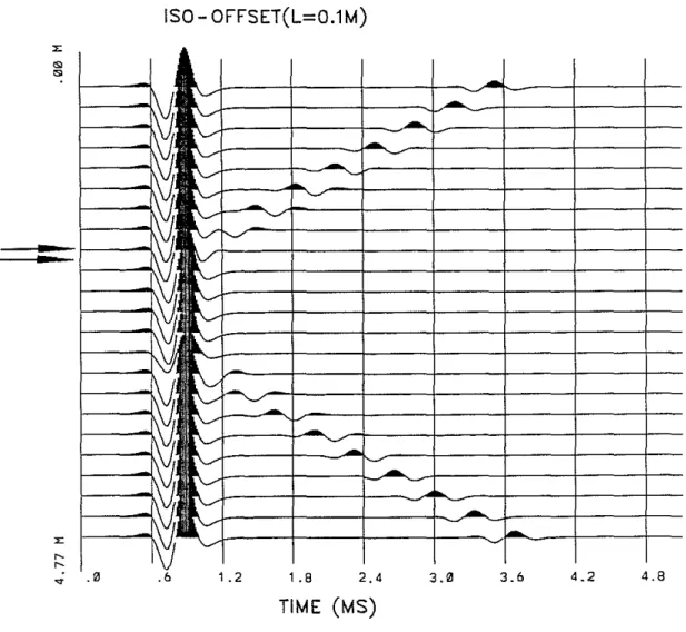
As a last example, we model the effects of a very thin fractured zone on the Stoneley wave propagation. This happens when the borehole penetrates a major geological fault. For the formation, we still use the same parameters as before. We assume that the fluid-saturated part of the zone is located in a thin layer of only 5 cm thick. For this thin layer, we further assume that the zone is filled with some loosely-spread materials, such as gravel, but is otherwise mostly saturated with fluid. For such fluid-solid mixture, we assume that the velocities and density of the solid are Vp =2.4 km/s, Vs =1.4 km/s, and p =2.1 kg/m3 . Since the layer is mostly filled with fluid, we assume a high porosity of

.p=70%

and a very high permeability of "0=300 Darcies. Such a high permeability can be measured from gravels (White, 1983). The saturant fluid is water whose properties have been given before. Since the effects of the fractured zone are the most significant at low frequencies and low-frequency logging tools have been available (Hornbyet aI., 1989), we use a source center frequency of 1 kHz in our modeling. The source-receiver spacing is 3 m. Figure 15 shows the synthetic seismograms. Because of the very high permeability and porosity, the very thin layer becomes a strong reflector and very significant Stoneley reflections are generated in this figure. In addition, the waves are attenuated across the fractured layer. Figure 16 plots the transmission and reflection coefficients for this case. The reflection coefficient here is the total reflection coefficient (Eq. 12) since the top and bottom reflection are indistinquishable for such a thin layer. The reflection coefficient is about 0.35 around 1 kHz. Reflection of this order has been measured by Hornby et al. (1989) for low-frequency waves at a major fracture. From this modeling, we see that a thin layer filled mostly with fluid and some loose materials acts qualitatively like a fluid-filled fracture, for the sum of the transmission and reflection coefficients is roughly 1, as in the planar fracture case (Tang and Cheng, 1988; Hornby et al., 1989). Because the solid materials in the fractured zone can sustain the overburden pressure, such a fluid-conducting channel is likely to exist in the field.

DISCUSSION

It is instructive to compare the single planar fracture theory studied previously and the fracture zone theory presented here. In the planar fracture theory, the sum of the transmission coefficient and the reflection coefficient is 1 (Tang and Cheng, 1988). This means that in order to produce the observed Stoneley amplitude attenuation (i.e., the transmission loss across the fracture) of about 60%, the reflection coefficient must be on the order of 0.6. However, Stoneley reflections from fractures with such a large amplitude have not been reported. Whereas Stoneley attenuation (>60%) acrossin situ fractures

24

Tang and Cheng

(

is frequently observed (Hardin et al., 1987; Paillet, 1980). Furthermore, for the planar fracture theory, such large attenuation or reflection requires that the fracture aperture be on the order of centimeters (see Figure 3). It is hard to imagine that fractures with such large apertures are still present under the in situ overburden pressure. For the permeable fracture zone theory, the overall magnitude of the reflection coefficient (top or total) is not sensitive to the thickness of the zone, while the transmission coefficient strongly depends on the thickness as well as the fluid-transport properties of the zone. Therefore, the transmission and reflection coefficients are not strongly correlated. This can be seen from Figure 14, where the transmission and reflection coefficients can both be small. This is consistent with field measurements in which strong transmission loss and small reflection both occur at permeable fractures (Paillet et aI., 1989). In addition, in the presence of multiple fractures, permeability or fluid transmissivity, rather than fracture aperture, is the appropriate parameter to characterize the overall fluid transport properties of fractures. Therefore, the permeable fracture zone model is a better theory than the planar fracture model in dealing with Stoneley propagation across fracture zones. However, this does not mean that the planar fracture model should be discarded. It can still be applied to cases where a single fracture is present. Infact, in the case of a very thin layer filled mostly with fluid, the fracture zone model and the planar fracture model are qualitatively similar, as has been shown in Figure 16. In addition, the study of the planar fracture case also gives us insight to our permeable fracture zone theory. As shown in Figure 4, the result of an inclined fracture dipping at 45° does not differ significantly from that of a horizontal fracture. Based on this observation, we can infer that for most practical cases involving permeable fracture zones dipping at less than

45",

it is sufficient to interpret the data in terms of the theory for a horizontal fracture zone.

SUMMARY AND CONCLUSIONS

We have formulated a simple theory that can be used to calculate Stoneley wave prop-agation across a variety of heterogeneous structures. Applying the theory to the case of a fluid-filled fracture, we found that our theory is fully consistent with the existing theory and accounts for the effect of the vertical extent of an inclined fracture. Inthe case of an elastic layer between two formations, reflections from both the top and the bottom interfaces are generated, which, when thickness of the layer is thin compared to the wavelength, may interfere constructively to produce an enhanced reflection, al-lowing the thin layer structure to be detected. Of primary importance are the cases of a permeable porous layer and a fracture zone. The theoretical results show that both the transmission and reflection of Stoneley waves are sensitive to the fluid transport properties of the zone. When the zone is highly permeable, Stoneley waves transmitted across the zone can be largely attenuated or even eliminated. This result is particularly significant in explaining the strong Stoneley wave attenuation observed at major frac-ture zones. Whereas it is very difficult to explain this strong attenuation in terms of the

plane-fracture theory. An important application of the fracture zone theory is to use it to model the observed Stoneley wave transmission and reflection at fracture zones. By matching the amplitudes of the transmitted and reflected waves, the overall fluid transmissivity of the zone can be assessed. Furthermore, because of the simplicity and efficiency in calculating the forward model, an inversion problem may be formulated based on the model, so that such parameters as permeability, porosity, and tortuosity of the zone can be estimated from the measured Stoneley wave data.

ACKNOWLEDGEMENTS

The authors would like to thank Denis Schmitt of Mobil for his helpful discussions. This research was supported by the Full Waveform Acoustic Logging Consortium at M.LT., by Department of Energy grant No. DE-FG02-86ER13636, and by New England Research, Inc.

REFERENCES

Bhashvanija, K., A finite difference model of an acoustic logging tool: The borehole in a

horizontal layered geologic medium,Ph.D. Thesis, Colorado School of Mines, Golden, CO., 1983.

Biot, M.A., Theory of propagation of elastic waves in a fluid-saturated porous solid, I: Low frequency range, J. Appl. Phys., 33, 1482-1498, 1956a.

Biot, M.A., Theory of propagation of elastic waves in a fluid-saturated porous solid, II: Higher frequency range, J. Acoust. Soc. Am., 28, 168-178, 1956b.

Cheng, C.H., J. Zhang, and D.R. Burns, Effects of in-situ permeability on the propaga-tion of Stoneley (tube) waves in a borehole, Geophysics, 52, 1297-1289, 1987.

Hardin, E.L., C.HjCheng, F.L. Paillet, and J.D. Mendelson, Fracture characterization by means of attenuation and generation of tube waves in fractured crystalline rock at Mirror Lake, New Hampshire, J. Geophys. Res., 92, 7989-8006, 1987.

Hornby, RE., D.L. Johnson, K.H. Winkler, and R.A. Plumb, Fracture evaluation using reflected Stoneley-wave arrivals, Geophysics,

54,

1274-1288, 1989.

Hornby, B.E., S.M. Luthi, and R.A. Plumb, Comparison of fracture apertures computed from electrical borehole scans and reflected Stoneley waves: an integrated interpre-tation, Tmns., SPWLA 31st Ann. Symp., Paper L, 1990.

26 Tang and Cheng

(

in fluid-saturated porous media, J. Fluid Mech., 176, 379-400, 1987.

Kelly, K.R, RW. Ward, S. Treitel, and RM. Alford, Synthetic microseismograms: A finite-difference approach, Geophysics, 41, 2-27, 1976.

Paillet, F.L., Acoustic propagation in the vicinity of fradures which intersect a fluid-filled borehole, Trans., SPWLA 21st Ann. Symp., Paper DD, 1980.

Paillet, F.L., and J.E. White, Acoustic modes of propagation in the borehole and their relationship to rock properties, Geophysics, 47, 1215-1228, 1982.

Paillet, F.L., C.H. Cheng, and X.M. Tang, Theoretical models relating acoustic tube-wave attenuation to fracture permeability - reconciling model results with field data,

Trans., SPWLA 30th Ann. Symp., Paper FF, 1989

Rosenbaum, J.H., Synthetic microseismograms: logging in porous formations, Geophysics,

39, 14-32, 1974.

Schmitt, D.P., Transversely isotropic saturated porous formations: II. wave propaga-tion and appliapropaga-tion to multipole logging, M.l. T. Full Waveform Acoustic Logging

Consortium Annual Report, 1988.

Schmitt, D P., M. Bouchon, and G. Bonnet, Full-waveform synthetic acoustic logs in radially semiinflnite saturated porous media, Geophysics, 53, 807-823, 1988.

Stephen, RA., F. Pardo-Casas, and C.H. Cheng, Finite difference synthetic acoustic logs, Geophysics, 50, 1588-1609, 1985.

Tang, X.M., and C.H. Cheng, A dynamic model for fluid flow in open borehole fractures, J. Geophys., Res., g4, 7567-7576, 1988.

Tang, X M., C.H. Cheng, and M.N. Toksoz, Dynamic permeability and borehole Stoneley waves: A simplified Biot-Rosenbaum model, submitted to J. Acoust. Soc. Am., 1990.

Tang, X.M., Acoustic logging in fractured and porous formations, Sc.D. Thesis,

Mas-sachusetts Institute of Technology, Cambridge, MA., 1990.

Tang, X.M., and C.H. Cheng, Effects of a logging tool on the Stoneley wave propa-gation in elastic and porous formations, M. I. T. Full Waveform Acoustic Logging

Consortium Annual Report, this issue, 1991.

White, J.E., Underground Sound, Elsevier Science Pub!. Co., Inc., 1983.

(

SOURCE BOREHOLE

FORMATION

LOGGING TOOL RECEIVER

Figure 1: Diagram showing acoustic logging across a borehole structure whose properties are different from those of the surrounding formation.

28 Tang and Cheng ( ( ( L

ntal

re

J

C

fracture

t

borehole

a. Horizo

Fractu

b. Inclined

Fracture

borehole

Figure 2: (a) A horizontal planar fracture of thickness L

_o

crossing the borehole. (b) Fracture of thickness L

_o

crossing the borehole at an angle B, making an elliptic hole (the shaded area) within the borehole. The vertical extent of the fracture within the borehole is L.

1

0.8

1 cm U.

--_

..

---UJ

----

---0

---

----()

--_

..

---

---0.6

---Z

---Q

en

en

_0.4

~

en

- - this study

Z

«

0.2

- - - - fracture theory 0::

I-0

0

0.5

1

1 . 5

2

FREQUENCY

(kHz)

Figure 3: Transmission coefficients for a Stoneley wave crossing horizontal fractures of different thicknesses. The results are calculated using Eq. (15) (solid curves) and Hornby et al. (1989) theory (dashed curves). The two theories compare very well.

30 Tang and Cheng

a

'EQUIVALENT CIRCLE' RESULT

0.25 0.2 u. UJ 0 () _0.15 Z 0 i= 0.1 () UJ .J U. UJ _0.05 a: G=Oo 0 0 0.2 0.4 0.6 0.8 FREQUENCY (kHz)

b

.25 a = 10 em d

=

0.3 em .20 c

=

1.5 km/s Ic(45°)

=

1200 Hz .15 Ic(700)

=

430 Hz I

r

I .10 8=70° .05 200 400 600 I(Hz) 800 1000

Figure 4: Theoretical values of the amplitude of the reflected waves from a fracture intersecting the borehole at various angles. (a) Results obtained from the present 'equivalent circle' approach. (b) Hornby et aL's (1989) results obtained using Math-ieu functions. The results from the two different approaches are in fairly good agree-ment. Note however, that in both (a) and (b) the vertical extent of the fracture is not accounted for.

0.25

total effects flow effects

--- ---

_---

_{- ...}

_--..

_--

..

_---

..

-0.1

0.2

0.05

0.15

u..

w

o

()

z

o

i=

() W ...J

u..

W

a:

o

o

0.2

0.4

0.6

FREQUENCY (kHz)

0.8

1

Figure 5: Amplitude of reflection coefficient at angles

e

=

45° and

e

=

70°, calculated with both the effect due to flow into an elliptical boundary and the effect due to the vertical extent of the fracture (solid curves). The results due to flow effects only are also shown (dashed curves), which are valid only below the frequencies indicated on Figure 4b.

32

•

•

.

~ .5

Tang and Cheng

T

TIME eMS)

B

I

BT

BTB

3.3 3.8 ( (

Figure 6: Synthetic S toneley array waveforms across an elastic layer of 50 em thick with different properties. The waves are largely enhanced and the high amplitudes are clipped to show the small reflection events. Multiple reflections are generated. The symbols are: I=incident wave, T=top boundary reflection, B= bottom bound-ary reflection, BT=secondbound-ary reflection at the top due to the reflection B, and BTB=refiection at the bottom due to the reflection BT. The location of the layer is indicated by arrows.

ISO - OFFSET(L=0.5M) 4.8 4.2 3.6 3.~ 2.4 1.8 1 .2 .~ f---I.v

~....I----+--+-~.J----+---+---1­

1 - - -....,v

\:.-1----1---+----+---1---+---+-1--_-\

,Y

;\---J.---I---1-- I l 1 I -i----l"v

Y

0...-1 - - - - \

'vlt:...-L...---+-...

I I + + I +

-r---+.-"

,~

:'v-\),

;\---.J----+---J...---l---+---+--+-I--~

':..;,

0----

\), ;\.J+J.+... + + +

-f - - - (

V,

0----f - - - {

'VI

;\---J---l---I---....-Jo--I---+--+--VI

;\---....I----I---!---I--...--!---....1'----11--I--~

'VI

0----J----+--I---+---k..----+----+--V,

"v..-l---+---+--+---!---+---+~--V .6

•

TIME (MS)

Figure 7: Synthetic iso-offset Stoneley wave seismograms across the elastic layer of 50 cm thick (indicated by arrows). The Stoneley arrivals are delayed across the layer of slower velocity. In particular, when the source passes through the layer, the emitted Stoneley waves become weaker due to the softer layer, as indicated on the

34 Tang and Cheng

a.

TOTAL REFLECTION 0.3 , - - - , ( --L=10cm 1 2 3 4 5 FREQUENCY (kHz)

u.

w

o

0.2 () Z

o

i= () W 0.1 ...J U. W

a:

o

."\

.I \

! \

!

i

i

o

/\

i

i

, i

\ :

: i

_\ : V -"'-L=50cm

! \.

'\

i '

.

\. ₍f \

!

'

.

\ i

\!

\ !

\

!

, i

' :

\:

_.,'

\ !

_V

r·.

.'

\

I " f

i

/

,

,

\

\

\

6 (

b. REFLECTION FROM TOP BOUNDARY

0 . 0 9 , - - - , --L=infinity ~- - - - L=10 em -···-L=50cm

u.

W

o

_~

_...

_=.d-2~~"'/"=.:.::-.=.7

..

"--': ...

_-_._----o

0.08 i= .,...:. () W ...J U. W

a:

.~

---o

1 2 3 4 5 FREQUENCY (kHz) 6

Figure 8: Characteristics of Stoneley wave reflection from elastic layers of different thicknesses. (a) total reflection. (b) top reflection only. The total reflection in (a) shows mainly the superposition of the top and bottom reflections. The periodic spectrum can be used to deduce the thickness of the layer. The top reflection in (b) shows that the overall magnitude of the top reflection coefficients for layers of different thicknesses are close to the reflection from the interface between two semi-infinite formations.

ISO - OFFSET(L=O.1M) 4.8 4.2 3.6 3.0 2.4 , .8 1.2 .6 .0 >: <Sl <Sl ..-[\.-- _~

':JJ

[\....

-~

~ L-.

-,V,

.-..

,v,

:'-'

-V,

-\J

1'----'

-

₀

-IV ,\, ,v

~

-.v

-..-v

K:

.--...-.

A10.

-.

,"

l-. >: _,'-' "-": v TIME (MS)

Figure 9: Synthetic iso-offset seismograms across a thin elastic layer of 10 cm thick (indicated by arrows). Because of the thin layer, the top and bottom reflections are inseparable and combine to give an enhanced reflection.

36

•

Tang and Cheng

POROUS ZONE(L=O.5M) I . . .oA'

...

_ 1&

- V/,..

~--+---_+--_!_--+_-_+-I---+----+-\v,,.-'

loI--+---+----+---t---t--+----+----t--___'

~

+ I + ! !

-'.

+--_ _+--_ _t--___

I

~

... + I I ! !

-I----+----t'"~

..

~j!ll---I---+---t---t----+-....

..

_...

..

..

_...

( ( ,0 .6 1 8 2.4 3.0 3.6 4.2 4.8 TIME (MS)

Figure 10: Iso-offset Stoneley waves across a permeable porous layer. The overall feature shown in this figure is that the wave amplitudes are significantly attenuated across the zone.

0.8

TRANSMISSION AND REFLECTION

AT A PERMEABLE POROUS ZONE

0.6

W transmission Q ::::l

t::

_0.4

total reflection - I

a..

~.I

1C =50

::

0

«

<1>=0.3

0.2

\

.

top reflection a=3

t

L=50 cm

...

.

..

0 0 2 4 6 8

FREQUENCY

(kHz)

Figure 11: Amplitudes of the transmitted and reflected waves from the porous zone. The transmission is only 0.45 around 3 kHz. The total reflection (dashed curve) periodically fluctuates around the top reflection (solid curve), because of the su-perimposition from the (weak) bottom reflection. The periodicity can be used to deduce the thickness of the layer.

(

38 Tang and Cheng

0.8 LL. LlJ

_0.6

0

U

Z

0

...

_

...

__

._--

..

_

...

-en

0.4

tortuosity=3

en

-:2

en

_tortuosity=1

:z

<C

0.2

0:

I-0

0

2

4

6

8

FREQUENCY

(kHz)

Figure 12: Effect of tortuosity a on the Stoneley transmission across a permeable zone. For both the fracture zone (a = 1), and the porous zone (a = 3), the transmission is close at low frequencies, but the fracture zone case shows more transmission loss at high frequencies.

•

•

FRACTURE ZONE(L=O.4M)

-

--'

"""

_{(Jil1~_-+-_-1-_-+-_-+_-+_}

If•.

I - - - + - - - l - " ' t' . l + I I I \

-~

_ _+-_-i""'1

~

...

~I~_-_-J.---1----1----!---+--

--

-'"

N N

'"

.0 .6

-

_IV

1.2 V 1 . S 2.4 3.0 3.6 4.2 4.8 TIME (MS)

Figure 13: Synthetic Stoneley wave seismograms across a permeable fracture zone. Note that significant Stoneley reflection and very strong Stoneley attenuation both occur at the fracture zone.

40

0.8

Tang and Cheng

TRANSMISSION AND REFLECTION

AT A FRACTURE ZONE

K O=20 D

0.6

_{<I> =0.4} total reflection W 0.=1 C L=40 cm

::>

I-

0.4

::i

a.

::::r:

transmission <C

0.2

top reflection

0

0

1 2

3

4

5

6 7 8

FREQUENCY

(kHz)

Figure 14: Amplitudes of the transmitted and reflected waves from the fracture zone. The transmission is only about 0.25 around 3 kHz. The reflections (total and top) have higher amplitudes than those of the porous zone case shown on Figure 11.

FRACTURE ZONE(L=5CM) _"-../ ~"-J ~V

...

~

JA:-~

-..

I---'

'--I

'--~

~

---..-~

....

...

-' - J

_.-.

' - _V

-"--'

'

-•

<Sl N .0 1.2 2.4 3.6 4.8 6.0 7.2 8.4 9.6 TIME (MS)

Figure 15: Stoneley seismograms in the vicinity of a very thin fracture zone filled largely with fluid (4)=70%). Note the strong reflections generated by this thin zone.

42

1

Tang and Cheng

0.8

LU

_0.6

l=5cm Cl K O=300 D

::::>

!::

<1>=0.7 ..J C.

0.4

(l=1

::

reflection

<l:

0.2

o

o

0.5

1

1.5

2

FREQUENCY

(kHz)

2.5

Figure 16: Transmission and reflection coefficients across the thin fracture zone. The behaviors of these curves are somewhat similar to those of a fluid-filled fracture. The sum of two curves is close to 1.