Publisher’s version / Version de l'éditeur:
Vous avez des questions? Nous pouvons vous aider. Pour communiquer directement avec un auteur, consultez la
première page de la revue dans laquelle son article a été publié afin de trouver ses coordonnées. Si vous n’arrivez pas à les repérer, communiquez avec nous à PublicationsArchive-ArchivesPublications@nrc-cnrc.gc.ca.
Questions? Contact the NRC Publications Archive team at
PublicationsArchive-ArchivesPublications@nrc-cnrc.gc.ca. If you wish to email the authors directly, please see the first page of the publication for their contact information.
https://publications-cnrc.canada.ca/fra/droits
L’accès à ce site Web et l’utilisation de son contenu sont assujettis aux conditions présentées dans le site LISEZ CES CONDITIONS ATTENTIVEMENT AVANT D’UTILISER CE SITE WEB.
Advances in Visual Computing: 5th International Symposium, ISVC 2009, Las
Vegas, NV, USA, November 30 - December 2, 2009, Proceedings, Lecture Notes
in Computer Science; no. 5875, pp. 586-595, 2009
READ THESE TERMS AND CONDITIONS CAREFULLY BEFORE USING THIS WEBSITE. https://nrc-publications.canada.ca/eng/copyright
NRC Publications Archive Record / Notice des Archives des publications du CNRC :
https://nrc-publications.canada.ca/eng/view/object/?id=3e2e5d55-2103-4229-993d-ee4bdc2531c1
https://publications-cnrc.canada.ca/fra/voir/objet/?id=3e2e5d55-2103-4229-993d-ee4bdc2531c1
NRC Publications Archive
Archives des publications du CNRC
For the publisher’s version, please access the DOI link below./ Pour consulter la version de l’éditeur, utilisez le lien DOI ci-dessous.
https://doi.org/10.1007/978-3-642-10331-5_55
Access and use of this website and the material on it are subject to the Terms and Conditions set forth at
Fast 3D reconstruction of the spine using user-defined splines and a
statistical articulated model
Moura, Daniel C.; Boisvert, Jonathan; Barbosa, Jorge G.; Tavares, João
Manuel R. S.
Fast 3D Reconstruction of the Spine Using
User-Defined Splines and a Statistical
Articulated Model
Daniel C. Moura1,2, Jonathan Boisvert5,6, Jorge G. Barbosa1,2, and Jo˜ao
Manuel R. S. Tavares3,4
1
Lab. de Inteligˆencia Artificial e de Ciˆencia de Computadores, FEUP, Portugal 2
U. do Porto, Faculdade de Engenharia, Dep. Eng. Inform´atica, Portugal 3
Instituto de Engenharia Mecˆanica e Gest˜ao Industrial, Campus da FEUP, Portugal 4
U. do Porto, Faculdade de Engenharia, Dep. de Eng. Mecˆanica Rua Dr. Roberto Frias, 4200-465 Porto, Portugal
{daniel.moura,jbarbosa,tavares}@fe.up.pt 5
National Research Council Canada, 1200, Montreal Rd, Ottawa, K1A 0R6, Canada 6 ´
Ecole Polytechnique de Montr´eal, Montr´eal, QC H3T 1J4, Canada jonathan.boisvert@nrc-cnrc.gc.ca
Abstract. This paper proposes a method for rapidly reconstructing 3D models of the spine from two planar radiographs. For performing 3D reconstructions, users only have to identify on each radiograph a spline that represents the spine midline. Then, a statistical articulated model of the spine is deformed until it best fits these splines. The articulated model used on this method not only models vertebrae geometry, but their relative location and orientation as well.
The method was tested on 14 radiographic exams of patients for which reconstructions of the spine using a manual identification method where available. Using simulated splines, errors of 2.2±1.3mm were obtained on endplates location, and 4.1±2.1mm on pedicles. Reconstructions by non-expert users show average reconstruction times of 1.5min, and mean errors of 3.4mm for endplates and 4.8mm for pedicles.
These results suggest that the proposed method can be used to recon-struct the human spine in 3D when user interactions have to be min-imised.
1
Introduction
Three-dimensional reconstructions of the spine are required for evaluating spinal deformities, such as scoliosis. These deformities have a 3D nature that cannot be conveniently assessed by planar radiography. Clinical indexes that may only be measured with 3D models include, for example, the maximum plane of curva-ture [1], but there are several others that cannot be accurately quantified using planar radiography, such as the axial rotation of vertebrae. On the other hand, 3D imaging techniques (i.e. Computer Tomography (CT) and Magnetic Reso-nance Imaging (MRI)) are not suitable because they require patients to be lying
down, which alters the spine configuration. Additionally, they are more expen-sive and, in the case of CT, the doses of radiation required for a full scan are too high to be justified for multiple follow-up examinations. For all those reasons, 3D reconstructions of the spine are usually done using two (or more) planar radiographs.
Three-dimensional reconstruction of the spine using radiographs is usually done by identifying a predefined set of anatomical landmarks in two or more radiographs. In [2] a set of 6 stereo-corresponding points per vertebra is required to be identified, and in [3] this set is increased even more to enable identifying landmarks that are visible in only one of the radiographs. These methods require expert users and, additionally, they are very time-consuming, error-prone and user-dependent. In [4] the time required by a user to reconstruct a 3D model was decreased to less than 20min by requiring a set of 4 landmarks per vertebra in each radiograph. However, this amount of user interaction is still high for clinical routine use.
Very recently, new methods are arising that try to reduce user interaction by requesting the identification of the spine midline on two radiographs, and make use of statistical data for inferring the shape of the spine. This is the case of [5] where, besides the splines, two additional line segments are needed for achieving an initial reconstruction. Then, several features are manually adjusted that are used along with the initial input for producing the final model. This processes requires an average time of 2.5min, although users may refine reconstructions, increasing interaction time to 10min. Kadoury et al. also proposed using a sta-tistical approach to obtain an initial model of the spine from two splines, which is then refined using image analysis [6]. However, this study only uses the spine midline as a descriptor to get the most probable spine shape for that midline. While this is acceptable, there may be a range of spine configurations for the same spline. Additionally, in both studies, the authors do not make a complete use of the user input, since the control points that the user marks for identify-ing the spine midline are ignored, while they may carry information about the location of some vertebrae. Finally, the statistical models of this studies do not conveniently explore the inter-dependency of position and orientation between vertebrae.
In this paper, we propose a method for reconstructing the spine from its midline that uses an articulated model [7] for describing anatomical variability. This model effectively represents vertebrae inter-dependency and it has already demonstrated capabilities for inferring missing information [8]. The model is then deformed using an optimisation process for fitting the spine midline while making use of all the information that the user inputs, that is, the location of the control points that define the midline are used for controlling the deformation of the statistical model.
Fast 3D Reconstruction of the Spine Using Splines and an Articulated Model 3
2
Methods
2.1 Articulated model of the spine
Statistical models of anatomical structures are often composed by a set of land-marks describing their geometry. In the case of the spine, this could be done by using a set of landmarks for each vertebra. However, the spine is a flexible structure. The position and orientation of the vertebrae are, therefore, not inde-pendent. Capturing the spine as a cloud of points does not differentiate vertebrae and, consequently, information is lost that may be important to capture spinal shape variability and vertebrae inter-dependencies.
For tackling this problem, Boisvert et al. proposed the use of articulated mod-els [7]. These modmod-els capture inter-vertebral variability of the spine geometry by representing vertebrae position and orientation as rigid geometric transforma-tions from one vertebra to the other along the spine. Only the first vertebra (e.g. L5) has an absolute position and orientation, and the following vertebrae are dependent from their predecessors. This may be formalised as:
Tiabs = T1◦ T2◦ · · · Ti, for i = 1..N, (1)
where Tabs
i is the absolute geometric transformation for vertebra i, Ti is the
geometric transformation for vertebra i relative to vertebra i − 1 (with the ex-ception of the first vertebra), ◦ is the composition operator, and N is the number of vertebra represented by the model.
In order to include data concerning vertebrae morphology, a set of landmarks is mapped to each vertebra in the vertebrae coordinate system, which has its origin at the vertebral body centre. The absolute coordinates for each landmark may be calculated using the following equation:
pabsi,j = T abs
i ⋆ pi,j, for i = 1..N, j = 1..M, (2)
where pabs
i,j are the absolute coordinates for landmark j of vertebrae i, pi,jare the
relative coordinates, ⋆ is the operator that applies a transformation to a point, and M is the number of landmarks per vertebra.
The method proposed on this paper uses an articulated model of the spine composed by N = 17 vertebrae (from L5 to T1) with M = 6 landmarks per vertebra (centre of superior and inferior endplates (j = 1..2), and the superior and inferior extremities of the pedicles (j = 3..6)).
2.2 User input
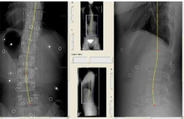
User input is limited to identifying the spine midline in two different views using parametric splines like illustrated by figure 1. Both splines should begin at the centre of the superior endplate of vertebra T1 and should end at the centre of the inferior endplate of L5. These are the only landmarks that must be present in both radiographs, all the other control points may be identified in only one radiograph without having a corresponding point in the other.
Fig. 1. Graphical user interface designed for defining the splines.
In order to impose restrictions concerning vertebrae location, users are asked to mark all the control points in the centre of the vertebral bodies (with the exception of T1 and L5). In fact, there is a natural tendency for users to place control points on the centre of vertebral bodies, even when not asked to, and this way splines also carry information about the location of some vertebrae.
2.3 Fitting the articulated model to the splines
For fitting the model to the splines, an optimisation process is used that iter-atively deforms the articulated model and projects the anatomical landmarks on both radiographs simultaneously, towards reducing the distance between the projected landmarks of the model and the splines. Principal Components Anal-ysis (PCA) is used for reducing the number of dimensions of the articulated model, while capturing the main deformation modes. Using PCA in a linearised space, a spine configuration x = [T1, . . . , TN, p1,1, . . . , pN,M], may be generated
using the following equation:
x= ¯x+ γd, (3)
where ¯xis the Frech´et mean of a population of spines represented by articulated models [7], γ are the principal components coefficients (calculated using the co-variance matrix of the same population), and d is the parameter vector that controls deformations. The absolute position of every landmark for any config-uration x may be obtained by applying equation 1 (for calculating the absolute transformations) and then equation 2.
The goal of the optimisation process is finding the values of d that generate the spine configuration that best fits the splines of both radiographs. For calcu-lating the distance between the articulated model and the splines, we propose projecting to both radiographs the landmarks of the articulated model that de-fine the spine midline. This midline may be represented as a subset of pabs where
Fast 3D Reconstruction of the Spine Using Splines and an Articulated Model 5
only the landmarks of the centres of endplates are used: q=©pabs
i,j : ∀i, j ∈ {1, 2}ª . (4)
From q, projections of the midline landmarks, q2D 1 and q
2D
2 , may be calculated
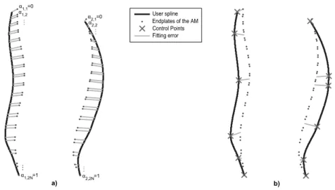
for the two calibrated radiographs respectively. This is illustrated on figure 2 where it is possible to see the user-identified splines and the projections of the spine midline of the articulated model for the two radiographs.
At this stage, the user input and the articulated model are in the same dimensional space (2D), and both may be represented by splines. However, it is not straightforward to quantify the distance between the two since the user splines may have a different length than the spine midlines of the articulated model (q2D
k ). For tackling this, we first project q 2D
k to the one dimensional space
defined by the spline that has q2D
k as control points and normalise this 1D
projections to the spline length. This may be formalised in the following way: αk,l= length(q2D k ,1, l) length(q2D k ,1, 2N ) for k = 1..2, l = 1..2N, (5) where length(q2D
k , a, b) is the function that calculates the length of the segment
of spline q2D
k delimited by control points a and b. Vector α is independent of the
spline length and, thus, it may be used for mapping the projected spine midlines of the articulated model with the splines identified by the user (figure 2a). This enables to define the following cost function:
C= 2 X k=1 2N X l=1 ° °qk,l2D− (sk⋄ αk,l) ° ° 2 , (6)
where sk represents the user spline for radiograph k, and ⋄ is the operator that
maps 1D normalised coordinates of a given spline to 2D coordinates. This func-tion is minimised using Matlab’s implementafunc-tion of the trust-region-reflective method [9] for nonlinear least-squares problems.
2.4 Optimising vertebrae location
The fitting process just presented only enables to capture the spine shape by placing vertebrae in their probable location along the spine midline, which may not be the correct one. For improving this issue without requesting additional information to the user, we make use of the location of the control points of the splines, which are placed at the centre of vertebral bodies (with the exception of the first and the last control points). Using this specific anatomical position enables us to know that there is a vertebra at the control point location. However, the vertebra identification is unknown, and, therefore, it is not possible to know for sure which vertebra in the articulated model should be attracted by a given control point.
For tackling this issue, after a first optimisation with the previously presented process, for each control point, the two nearest vertebrae of the articulated model
Fig. 2. Fitting the articulated model to the splines: a) The spine midline of the 3D articulated model (AM) is projected to both radiographs (frontal and lateral). The 1D normalised coordinates (α) of the landmarks that compose the 2D spine midline are used for mapping the articulated model with the user splines. b) Control points attract the nearest vertebra of the articulated model (each vertebra is represented by the centre of its endplates, with the exception of T1 and L5).
are selected as candidates. Then, the nearest candidate is elected if the level of ambiguity is low enough. This may be formalised on the following way:
2dm,1
dm,1+ dm,2
≤ ω, (7)
where dm,1 is the distance of control point m to the nearest candidate of the
articulated model, dm,2 is the distance to the second nearest candidate, and ω
is a threshold that defines the maximum level of ambiguity allowed. Ambiguity takes the value of 1 when the candidates are equidistant to the control point (total ambiguity), and takes the value of 0 when the nearest candidate is in the exact location of the control point (no ambiguity).
After determining the set of elected candidates, E, the optimisation process is repeated, but now including a second component that is added to equation 6 that attracts the elected vertebrae of the articulated model towards their corre-spondent control points (figure 2b):
C= 2 X k=1 2N X l=1 ° °q2k,lD− (sk⋄ αk,l) ° ° 2 + X m∈E kdm,1k 2 . (8)
When the second optimisation finishes, the vertebrae location of the articu-lated model should be closer to their real position, and some of the ambiguities may be solved. Therefore, several optimisation processes are executed iteratively while the number of elected candidates, E, increases.
Fast 3D Reconstruction of the Spine Using Splines and an Articulated Model 7
Concerning the value of ω, using a low threshold of ambiguity may result in a considerable waste of control points due to an over-restrictive strategy. On the other hand, a high threshold of ambiguity may produce worst results, especially when there are control points placed on erroneous locations. For overcoming this issue, a dynamic thresholding technique is used that begins with a restric-tive threshold (ω = 0.60), and when no candidates are elected the threshold is increased (by 0.10) up to a maximum threshold of ambiguity (ω = 0.80). If there are any control points still ambiguous at this stage, they are considered to be unreliable.
3
Experiments and Results
For all experiments a data set of 14 in vivo exams of scoliotic patients was used. All exams were composed of at least one posterior-anterior (PA) and one lateral (LAT) radiograph. The 6 anatomical landmarks were previously identified on both PA and LAT radiographs by an expert and 3D reconstructions of the land-marks were available. These reconstructions were obtained using a previously validated method [10] and were used as reference on this study.
The articulated model that was used in all experiments was built using 291 exams. The principal components that explained 95% of the data variability were extracted, resulting in a model with 47 dimensions.
3.1 Evaluation using simulated splines
The first experiment consisted of evaluating the proposed method using perfectly marked splines for determining the expected error in ideal conditions. For this, splines with 6 control points were built using the available 2D hand-marked points. In particular, the centre of the superior endplate of T1 (first control point of splines) and the centre of the inferior endplate of L5 (last control point) were copied from the original 2D points. Then the centre of the vertebral body of the remaining vertebrae was calculated using the average location of the centres of both endplates. Finally, for each exam, and for each radiograph, 4 vertebral body centres were selected as control points of the spline in order to best fit all the endplates’ centres that were manually identified by an expert. Reconstructions with these splines resulted on an error of 2.2±1.3mm for the endplates and 4.1±2.1mm for pedicles (mean ± S.D.).
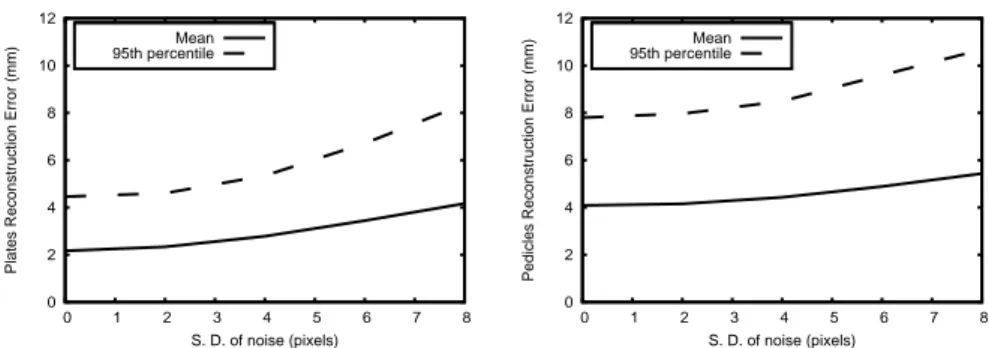
For determining the effect of identification errors of the control points on the quality of reconstructions, a second experiment was made where Gaussian noise with standard deviation up to 8 pixels was introduced to the 2D coordinates of the control points. Results of this experience are presented in figure 3.
3.2 Evaluation using manually identified splines
The last experience concerned evaluating the method performance when using splines manually identified by non-experts. For conducting it, 2 volunteers with
0 2 4 6 8 10 12 0 1 2 3 4 5 6 7 8
Plates Reconstruction Error (mm)
S. D. of noise (pixels) Mean 95th percentile 0 2 4 6 8 10 12 0 1 2 3 4 5 6 7 8
Pedicles Reconstruction Error (mm)
S. D. of noise (pixels) Mean
95th percentile
Fig. 3. Effect of simulated Gaussian noise added to the 2D location of the control points of the splines (reconstruction errors for: left – endplates; right: – pedicles).
very limited knowledge of the spine radiological landmarks marked the same 14 exams that were used in the previous experiments. Both of them only had 20min of training with the software tool before performing the experiment. Results of this experiment are presented in table 1, including the average time needed for a reconstruction. The presented times are dominated by user interaction since the average processing time is approximately 10s (on a Pentium Dual Core of 1.86 GHz). Additionally, the input error of each spline was calculated in two ways: a) Spline error: the distance between every endplate centre of the 2D reference data and the nearest point of the spline, and b) Control Points error: the distance between the control points coordinates and their ideal location. Figure 4 shows reconstructions of the proposed and reference methods for an average case.
4
Discussion and Conclusion
The method proposed here achieves 3D reconstructions of the spine by only requiring the identification of two splines by an user. Results with simulated splines composed by 6 control points were compared with the reference method, which needs 102 points per radiograph to be manually identified. The proposed method showed errors near of the in vitro accuracy of the reference method [10]
Table 1. Results for the experiment with splines identified by non-experts with 20min of training. Mean values (± S.D. for input and reconstruction errors). Number of C.P. is the average number of control points used for identifying the splines.
User Number Input error (pixels) Reconstruction Reconstruction Error (mm) of C.P. Spline C.P. Time (min:s) Endplates Pedicles A 6.1 6.3±5.7 5.9±5.4 1:22 3.4±1.9 4.8±2.5 B 5.5 5.2±5.0 8.7±8.6 1:32 3.4±2.0 4.8±2.6
Fast 3D Reconstruction of the Spine Using Splines and an Articulated Model 9
Fig. 4. Comparison of a reconstruction using the proposed method (solid line) with the reference method (dashed line) for an average case of manual identification by non-experts (endplates error– 3.2mm; pedicles error – 4.8mm).
for the endplates (2.2±1.3mm vs 1.5±0.7mm), but higher errors for pedicles (4.1±2.1mm vs 1.2±0.7mm). We believe that this happens because there is no direct input from the user concerning the localisation of pedicles, and therefore pedicles position and vertebrae axial rotation are completely inferred from the spine curvature.
Simulations considering artificial noise (figure 3) show a robust behaviour with a standard deviation of the noise up to 4 pixels. After this, the curve becomes steeper, especially on the 95th percentile of the endplates error. It is
also visible that identification errors have an higher impact on the accuracy of the endplates position than on pedicles, which is natural since the endplate position is much more dependent of the user input. Nevertheless, reconstruction errors of the endplates with noise of 8 pixels are comparable to pedicle errors with no noise.
Experiments with non-expert users revealed an average user time inferior to 1.5min, which is an advance in comparison with the previous generation of reconstruction algorithms. Reconstruction errors are mainly influenced by the quality of the user input either on the accuracy of the spline midline (higher on user A), or in the identification of the precise location of the control points (mainly on user B). In spite of this variability on the dominant source of error, reconstruction errors were comparable for both users. These errors are not com-parable with reconstructions performed by experts, but show that a rough initial estimation is at the reach of ordinary users. This is especially visible on figure 4 where it is noticeable that despite the visible input error, vertebrae location is quite accurate given the small amount of user input. Additionally, using more than one user on this experiment gives more credibility to the obtained results, and the fact that reconstruction errors were very similar for both users makes us believe that these results may be generalised. Future work will include thorough tests with even more users to reinforce these conclusions.
We believe that in future assessments of the method with an expert user, the results will be closer to the results achieved with simulated splines. Additionally, using more control points may improve the location of endplates, which creates a tradeoff between accuracy and user interaction. However, additional information will be needed for accurately locating pedicles. Future work includes determining the impact of knowing the location of small sets of pedicles landmarks, which may be either identified by users or by image segmentation algorithms.
Acknowledgements
The first author thanks Funda¸c˜ao para a Ciˆencia e a Tecnologia for his PhD scholarship (SFRH/BD/31449/2006), and Funda¸c˜ao Calouste Gulbenkian for granting his visit to ´Ecole Polytechnique de Montr´eal. The authors would like
References
1. Stokes, I.A.: Three-dimensional terminology of spinal deformity. a report presented to the scoliosis research society by the scoliosis research society working group on 3-d terminology of spinal deformity. Spine 19 (1994) 236–248
2. Aubin, C.E., Descrimes, J.L., Dansereau, J., Skalli, W., Lavaste, F., Labelle, H.: Geometrical modelling of the spine and thorax for biomechanical analysis of scoli-otic deformities using finite element method. Ann. Chir. 49 (1995) 749–761 3. Mitton, D., Landry, C., Vron, S., Skalli, W., Lavaste, F., De Guise, J.: 3d
recon-struction method from biplanar radiography using non-stereocorresponding points and elastic deformable meshes. Med. Biol. Eng. Comput. 38 (2000) 133–139 4. Pomero, V., Mitton, D., Laporte, S., de Guise, J.A., Skalli, W.: Fast accurate
stereoradiographic 3d-reconstruction of the spine using a combined geometric and statistic model. Clin. Biomech. 19 (2004) 240–247
5. Humbert, L., Guise, J.D., Aubert, B., Godbout, B., Skalli, W.: 3d reconstruction of the spine from biplanar x-rays using parametric models based on transversal and longitudinal inferences. Med. Eng. Phys. in press (2009)
6. Kadoury, S., Cheriet, F., Labelle, H.: Personalized X-Ray 3D Reconstruction of the Scoliotic Spine From Hybrid Statistical and Image-Based Models. IEEE Trans. Med. Imaging in press (2009)
7. Boisvert, J., Cheriet, F., Pennec, X., Labelle, H., Ayache, N.: Geometric variability of the scoliotic spine using statistics on articulated shape models. IEEE Trans. Med. Imaging 27 (2008) 557–568
8. Boisvert, J., Cheriet, F., Pennec, X., Labelle, H., Ayache, N.: Articulated spine models for 3-d reconstruction from partial radiographic data. IEEE Trans. Biomed. Eng. 55 (2008) 2565–2574
9. Coleman, T.F., Li, Y.: An interior trust region approach for nonlinear minimization subject to bounds. SIAM J. Optim. 6 (1996) 418–445
10. Aubin, C., Dansereau, J., Parent, F., Labelle, H., de Guise, J.A.: Morphometric evaluations of personalised 3d reconstructions and geometric models of the human spine. Med. Biol. Eng. Comput. 35 (1997) 611–618
to express their gratitude to Lama Seoud, Hassina Belkhous, Hubert Labelle and Farida Cheriet from Hospital St. Justine for providing access to patient data and for their contribution on the validation process.