Backroom space allocation in retail stores

(1)

Backroom space allocation in retail stores

by

Lita Das

B.E. (Hons), Mechanical, Birla Institute of Technology and Science (2009) M.Eng., Mechanical, Cornell University (2010)

S.M., Engineering Systems, Massachusetts Institute of Technology (2013) Submitted to the Institute for Data, Systems, and Society

in partial fulfillment of the requirements for the degree of Doctor of Philosophy in Engineering Systems

at the

MASSACHUSETTS INSTITUTE OF TECHNOLOGY

September 2018

@

Author ...

Signature redacted

Certified by...

Certified by.

...

Insti6te for Data, Systems, and Society

Signature redacted

August 22, 2018

Signature r

P, P

Signature

Certified by.. Certified by.. Accepted by ...

Signature

...

Yossi Sheffi Elisfa Gray II Professor of Engineering Systems Pyfesg of Civil and Environmental Engineering

edacted

Doctoral Committee Chair

...

Christopher Caplice rincipal Research Scientist and Executive Director Center for Transportation and Logistics

,-ed

acted

Thesis Supervisor

...

Karen Zheng Associate Professor, Sloan School of Management

redacted

Doctoral Committee Member Andre Carrel Assistant Professor, Civil, Environmental & Geodetic Engineering The Ohio State University /3 cl-Doctoral Committee Member

....

Signature redacted

...

Stephen Graves Abraham J. Siegel Professor of Management Science Professor of Mechanical Engineering Graduate Officer, Institute for Data, Systems and Society

MASSACHUSETTS INSTITUTE OF TECHNOWGY

w

OCT 3

62018

-4

.

(2)

(3)

Backroom space allocation in retail stores by

Lita Das

Submitted to the Institute for Data, Systems, and Society on August 22, 2018, in partial fulfillment of the

requirements for the degree of Doctor of Philosophy in Engineering Systems

Abstract

Space is one of the most scarce, expensive, and difficult to manage resources in urban retail establishments. A typical retail space broadly consists of two areas, the customer facing frontroom area and the backroom area, which is used for inventory storage and other support activities. While frontrooms have received considerable amount of attention from both academics and practitioners, backrooms are an often neglected area of retail space management and design.

However, the allocation of space to the backroom and its management impact multiple operational aspects of retail establishments. These include in-store labor utilization, de-livery schedules, product packaging, and inventory management. Therefore, the backroom area directly affects the performance of the store because it impacts stock-outs, customer service levels, and labor productivity. Moreover, extant literature suggests that backroom related operations contribute to a large fraction of the total retail supply chain costs. Thus, optimizing the management of backroom spaces is an important lever for store performance improvement.

We address the gap in the extant literature related to space management of retail back-rooms by investigating the following three questions: First, what is the effect of pack size on inventory levels and space needs in the backroom? Second, how can a given backroom space be efficiently utilized through optimal inventory control? Third, what is the optimal amount of space that should be allocated to the backroom in a given retail establishment?

To address the first question, we evaluate the effect of two discrete pack sizes, order pack size (OPS) and storable pack size (SPS), on inventory levels and storage space requirements in the backrooms. While SPS drives the space needs for a given inventory level,

OPS

drives the amount of excess inventory and therefore, the space needs. Using inventory theory and probability theory, we quantify the amount of excess inventory and the expected stock-out probability for a given OPS in the case of a normally distributed demand.

To address the second question, we discuss an inventory-theoretic approach to efficiently manage a given backroom space within a limited service restaurant. Specifically, we for-mulate a mathematical optimization model using mixed-integer linear programing with the objective of maximizing store profit. Applying this optimization model to real store data in collaboration with a major US retailer reveals cost implications related to constrained backroom space and the sensitivity of backroom space requirements to changes in OPS and SPS. The proposed model can serve as a decision support tool for various real-world use cases. For instance, the tool can help the retailers to identify (i) items whose contribution to the store profit does not justify their space needs in the backroom, and (ii) stores that are constrained in their profitability growth by backroom space limitations.

(4)

To address the third question, we introduce the notion of interdependency between the frontroom and the backroom of a retail establishment. Such interdependencies yield non-trivial trade-offs inherent to the optimal retail space allocation. Demand can be lost due to unavailability of inventory (or inventory stock-out), which is a result of scarce amount of backroom space, or due to unavailability of sufficient frontroom space (or space stock-out). Furthermore, constrained backroom spaces increase in-store labor cost and the ordering costs incurred per unit of revenue generated in a retail establishment. The strategic decision model formulated in this chapter accounts for revenue, inventory cost, labor cost and ordering cost to determine the optimal amount of backroom space that should be allocated within a retail establishment. Sensitivity analyses with respect to the change in input parameters is used to connect the backroom space allocation and its impact on store profit to the different supply chain levers that can be managed by the retailers.

Doctoral Committee Chair: Yossi Sheffi

Title: Elisha Gray II Professor of Engineering Systems Professor of Civil and Environmental Engineering

Thesis Supervisor: Christopher Caplice

Title: Principal Research Scientist and Executive Director Center for Transportation and Logistics

Doctoral Committee Member: Karen Zheng

Title: Associate Professor, Sloan School of Management

Doctoral Committee Member: Andre Carrel

Title: Assistant Professor, Civil, Environmental & Geodetic Engineering The Ohio State University

(5)

Acknowledgments

I am extremely grateful to my mentors, teachers, family, friends, and colleagues for their support throughout a tremendous academic journey at MIT.

First and foremost, I want to thank my advisor, Chris Caplice. I am deeply indebted to him for his guidance, support, patience, and encouragement. This thesis has immensely benefited from Chris's unparalleled expertise in supply chains. The enlightening and insight-ful discussions with him motivated me to conduct rigorous research as well as to investigate the questions from new perspectives that I would not have thought of otherwise. I greatly appreciate the freedom that he provided, which allowed me to explore different aspects and new boundaries of the research. I am also thankful for his instructions and feedback on how to effectively communicate my research work to both academic and industry audience, for giving me the opportunity to work for the revolutionary MicroMasters in Supply Chain Management program, and for never letting me worry about funding during my PhD. Thank you to my doctoral committee chair, Yossi Sheffi, for the invaluable advice, support, and insights on my research. I admire how he thinks both as an academic scholar as well as an industry expert. I hope that in the future I am able to emulate some of those qualities during the course of my career. Besides research guidance, I am privileged to have been taught, by Chris and Yossi, about the exciting world of supply chains - starting from the level of a SKU up to multi-echelon networks-through their lectures and discussions during in-class sessions and beyond. This laid the foundation for the directions that I took in my PhD research.

Thank you to my committee member, Karen Zheng, for all her support and asking intriguing questions that have encouraged me to think critically. I also want to thank Andre Carrel for helpful discussions both during our industry project collaborations at MIT Center for Transportation and Logistics (CTL) and later as my committee member, for detailed comments on my papers, and for teaching me different techniques for managing large datasets. I am also thankful to my industry partner for participating in interactive discussions that helped me understand the research topic from the practitioner's point of view.

During the course of my graduate program, I have learned a great deal from other faculty members at MIT. Thank you especially to Professors Joe Sussman, Chris Magee,

(6)

Richard Larson, Lisa D'Ambrosio, Oli de Weck and Richard de Neufville for teaching me the concepts of engineering systems (ES) through various lectures that were a part of the ES PhD curriculum. The stimulating class discussions convinced me of the power of inter-disciplinary research and taught me how to tackle large-scale complex systems. I also want to acknowledge Professors John Tsitsiklis, Roy Welsch, Robert Freund, and Retsef Levi for teaching me the methodologies that I used in my research.

I consider myself lucky to be a part of the Engineering Systems Division (now IDSS) and CTL communities. At CTL, I found an amazing support system-comprising of both researchers and administrative staff- that helped me tremendously through my PhD. I am forever grateful for all the help. Thank you to all CTL researchers for interesting and helpful discussions during individual sessions as well as research presentations and sharing their knowledge with me on various supply chain topics. A special thank you to Edgar Blanco for the pivotal discussions on the research and the support during the initial stage of my PhD. Thank you to Francisco Jauffred for always having his door open to engage in discussions related to inventory management topics. Thank you to Jim Rice for encouraging me, especially during the last leg and the most stressful part of the journey and to Eva Ponce for having made my work with the MicroMasters team enjoyable. I also want to acknowledge CTL administrative staff members, who have made things easier during this tough journey. Thank you to Nancy Martin, Mary Mahoney, Karen van Nederpelt, Tom Coveney, Arthur Grau, Eric Greimann, Christine Adams, and Katie Date. I am grateful to Beth Milnes, from IDSS, for her support and patience through the entire time here at MIT. I want to extend my gratitude to my wonderful friends, and fellow PhD students who I have interacted with, both for research related discussions as well as during numerous social events. Thank you to current and former colleagues: YinJin Lee, Atikhun Unahalekhaka, Alexandre Jacquillat, Maite Pena Alcaraz, Goksin Kavlak, Morgan Edwards; Abby Horn, Daniel Merchan, Andre Snoeck, Esteban Mascarino, Peter Zhang, Milena Janjevic, Stephen Zoepf, Angie Acocella, Michael Windle, Shraddha Rana, and Mohammad Moshref Javadi, who have made my time at MIT memorable. I am also grateful to my supportive friends outside of MIT who have helped me during difficult times, especially Bilhuda Rasheed, Ammar Tareen, Daniela Field, Rani Manoharan, Mikhil Ranka, my beloved Lopez family, Claire Jacquillat, and friends from BITS. I cherish our time together.

(7)

Mohanty, who is the biggest source of strength in my life- thank you for constantly encour-aging me to dream big, to think about what I can do to give back to humanity, and telling me that it is possible to achieve anything with hard-work, dedication, and determination. These are the guiding principles of my life. I want to thank my father, Girija Sankar Das, for all his love, which has kept me going through this arduous journey. Thank you to my brilliant, loving, supportive, and inspiring sister, Liza Das. I am in awe of her accomplish-ments and have considered her to be a role-model since a very young age. I also want to thank my aunt, Nirupama Meier and extended family in Bhubaneswar, who have been an integral part of my life since childhood, for all their love and support. Finally, to my partner, Matthias Winkenbach, who I adore- thank you for the unconditional love, tireless efforts to help me during this strenuous PhD journey, inspiring me by being an exemplary researcher in our field, engaging in useful and spirited discussions with me, and most importantly for being a big source of my happiness. I hope that we keep sharing beautiful adventures in life together.

(8)

To

(9)

OPS

equal to 1 . . . 46

2.4.2 Expected number of stock-out in units . . . 49

2.4.3 Implied adjustment to the planning safety stock level due to OPS constraint . . . 50

2.5 Trade-off between the excess space requirement and the reduction in expected probability of stock-out due to OPS effect . . . 51

2.6 The effect of SPS on space . . . 53

2.7 C onclusion . . . 54

2.8 A ppendix . . . 56

2.8.1 Derivation of expected probability of stock out . . . 56

2.8.2 Expected number of stock outs . . . 57

2.8.3 Proof of the distribution of un-truncated ending inventory distribution 58 2.8.4 Beginning inventory distribution from simulation . . . 59

2.8.5 Trade-off between the space requirement and expected probability of stock-out due to OPS effect: additional examples . . . 61

3 Improving the profit of a retail establishment through optimal backroom inventory control 62 3.1 Introduction . . . 62

3.2 Literature review on the effect of retail backroom space on store performance 65 3.3 Case study for the research . . . 67

3.4 Description of the specific research problem . . . 68

3.4.1 Problem setting . . . 69

3.4.2 Analysis framework . . . 70

3.5 Discussion of the different sub-models of the optimization model . . . 71

3.5.1 Accounting for the effect of pack sizes in the analysis . . . 71

3.5.2 Sub-model for demand translation process . . . 73

(11)

3.5.4 Sub-model for waste . . . 74

3.6 Optimization model . . . 75

3.6.1 Overview of the optimization model . . . 75

3.6.2 Additional notations . . . . 77

3.6.3 Optimization model . . . 78

3.6.4 Derivation of the objective function . . . 80

3.6.5 Constraints of the optimization model . . . 83

3.7 R esults . . . 84

3.7.1 Annual expected profit obtained with a given backroom space . . . 86

3.7.2 The cost of a constrained backroom space in a LSR . . . 88

3.7.3 The effect of pack sizes on the performance of a LSR with a constrained backroom space . . . 91

3.7.4 Can we infer the appropriate amount of backroom space that should be allocated from the model results? . . . 95

3.8 Conclusion and future research . . . 97

3.9 A ppendix . . . 98

3.9.1 Average order quantity and inventory on-hand under a (R,S) replen-ishm ent policy . . . 98

3.9.2 Derivation for the expected units sold . . . 100

3.9.3 Linearizing the loss function . . . 101

3.9.4 Accounting for the defrosting process to derive the effect on the service level for the frozen end-items . . . 102

4 Strategic allocation of backroom space in a retail establishment 4.1 Introduction . . . . 4.2 Relevant frontroom space related considerations in literature . . . . . 4.3 Effect of the frontroom and backroom on store profit . . . . 4.3.1 Hypothesis for revenue . . . . 4.3.2 Hypothesis for labor cost . . . . 4.3.3 Hypothesis for ordering cost . . . . 4.3.4 Hypothesis for inventory cost . . . . 4.4 Model formulation . . . . 106 . . . 106 . . . 109 . . . 110 . . . 112 . . . 114 . . . 116 . . . 117 . . . 117

(12)

4.5 Data used for analysis . . . . 4.5.1 Data related to space in the retail establishments . . . . 4.5.2 Other (non-space related) data for the retail establishments . . . 4.6 Estimated functional forms of the four profit components . . . . 4.6.1 Revenue as a function of the frontroom and backroom spaces in retail establishm ent . . . . 4.6.2 Inventory cost as a function of space . . . . 4.6.3 Estimated functional form for labor cost . . . . 4.6.4 Estimated functional form for ordering cost . . . . 4.7 Optimization model for strategic decision of backroom space allocation

retail establishm ent . . . . 4.8 Solving for backroom space . . . .

4.9 Sensitivity analysis . . . . 4.9.1 Sensitivity to the change in total retail space . . .

4.9.2 Sensitivity to the change in labor and ordering cost

4.9.3 Sensitivity to the change in inventory cost . 4.9.4 Effect of population density and store type profit . . . . 4.9.5 Comparison of sensitivity of the backroom

change in the regression parameters . . . .

4.10 Conclusion and future research . . . . 4.11 Appendix . . . .

5 Conclusion

5.1 Summary of research discussions 5.2 Future research ... .. ... th in 119 119 121 122 e 122 126 128 130 a 132 135 . . . 138 . . . 138 . . . 140 145 on space allocation and

. . . .

space allocation to the

147 . . . 149 . . . 154 . . . 157 158 . . . 158 ... ... ... .164

(13)

List of Figures

1-1 The functional areas in a retail establishment of a LSR . . . 20 2-1 Histogram for order pack size at Deltaco . . . 29 2-2 Histogram for ratio of storable pack size to order pack size at Deltaco . . . 29 2-3 An example to illustrate the effect of order pack size on amount of inventory

carried.

o=100

units/case, A=80 units/week and R = 1 week. In this case m = 20. . . . 33 2-4 Probability distribution for ending inventory of analytical method and from

sim ulation. . . . 40 2-5 Probability distribution of analytical method and from simulation for

begin-ning inventory. . . . 41 2-6 Comparing the results obtained from the formula and simulation-Normal. . . 44 2-7 Probability of stock-Out over different scenarios of variability. The figure

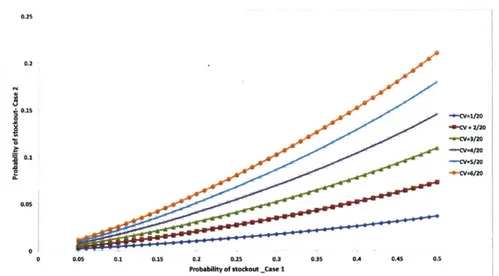
shows results for normally distributed demand with a mean of 20 units over a review period. The OPS is set at 12 units. . . . 47 2-8 Probability of stock out over different scenarios of order pack size (OPS).

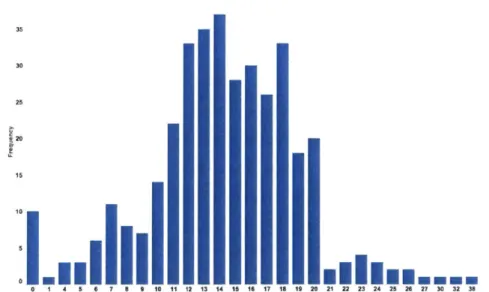
The figure corresponds to results run for normally distributed demand with a mean of 20 units and a standard deviation of 6. . . . 48 2-9 Empirical demand distribution of a SKU in a retail store of Deltaco . . . 48 2-10 Comparing Pr(SO) in cases

1

and 2 for an empirical demand distribution . . 49 2-11 Expressing (a) E[SO(units)IOPS > 1] as a percentage of E[SO(units)IOPS =

1] and (b) [CSLIOPS > 1] as a percentage of [CSL IOPS = 1]. The figure corresponds to results for a normally distributed demand with a mean and standard deviation of 70 and 15 units respectively. The order-up-to level is set at 80 units . . . 50

(14)

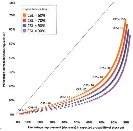
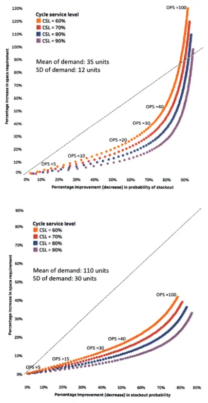
2-12 Percentage decrease in stock out probability vs. increase in space requirement

for an empirical distribution with different cycle service level . . . 53

2-13 Histogram for beginning inventory with deterministic demand . . . 59

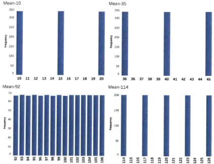
2-14 Histogram for beginning inventory with normally distributed demand . . . 60

2-15 Illustrations for trade-off for space requirement and stock-out probability . . 61

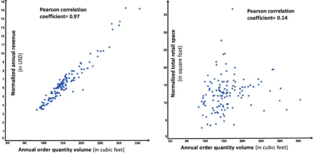
3-1 Backroom cubic volume flow through a store is positively correlated with the revenue generated to a considerable extent. . . . 66

3-2 Small retail space (thus typically a small backroom) does not mean smaller SKU volume flow through the store/backroom . . . 66

3-3 Different types of SKUs and end-items in Deltaco . . . 68

3-4 Framework of the optimization model . . . 71

3-5 Description of the characteristics of the 30 LSRs of Deltaco in the Mas-sachusetts region . . . 86

3-6 Illustration of the effect of constrained backroom space in a LSR: Expected profit change in SID_19 . . . 89

3-7 The change in the service level of the end-items (7j) with increase in the backroom space available . . . 90

3-8 Change in annual expected profit with change in

OPS

and SPS of a SKU . . 93

3-9 Change in the service level of the end-items (y7j) when SPS is changed to one for paper SKUs only. . . . 94

3-10 Comparison of the suggested and the current backroom space allocation in the stores when accounting for only inventory related cost . . . 96

4-1 The functional areas in a retail establishment of a LSR . . . 107

4-2 Revenue hypothesis. TR is the total store space . . . 114

4-3 Labor cost hypothesis . . . 116

4-4 Ordering cost hypothesis . . . 116

4-5 Total retail space vs. frontroom space in the observed stores . . . 120

4-6 Distribution of the implied frontroom to backroom ratio in our dataset of 122 stores . . . 121

4-7 Revenue per unit total retail (TR) space and the ratio of frontroom (FR) to backroom (BR) space . . . 123

(15)

4-8 Estimated revenue function for retail establishments of different sizes and for a given population density and store type . . . 125 4-9 Relationship between COGS and Revenue in our dataset . . . 127 4-10 Labor cost(LC) incurred to generate a unit of revenue (Rev) per unit total

retail space (T R ) . . . 130 4-11 Ordering cost (OC) incurred to generate a unit of revenue (Rev) per unit

total retail space (TR) . . . 132 4-12 Profit, Revenue and cost functions for a 1,600 sq.ft. retail establishment with

an average population density and walk-in only store type . . . 136 4-13 Comparison of the current BR space allocation to the results from the model

solution for individual stores . . . 138 4-14 Optimal BR space allocation in different types of LSRs for increasing total

retail space . . . . ... . . . 139

4-15 The change in the profit components in the different sized retail spaces . . . .140

4-16 Illustration of two scenarios for the ratio of labor cost to revenue across all stores ... ... ... ... .. .. ... ... .. 141 4-17 Sensitivity of optimal BR space and profit to change in the ratio of labor cost

to revenue . .. . . . . . . 143 4-18 Sensitivity of optimal BR space and profit to change in the ratio of ordering

cost to revenue ... ... 144 4-19 Estimated change in optimal BR space with change in ratio of COGS to

revenue . . . 145 4-20 Illustrating the change in the profit components with change in the ratio of

COGS to revenue . . . 146 4-21 Estimated change in optimal BR space and profit with change in ambient

population density . . . 148 4-22 Estimated change in optimal BR space and profit with change in store type . 149 4-23 Change of revenue with space dependent regression parameters . . . 151 4-24 Comparison of sensitivity of the optimal backroom space to space related

profit function parameters that are estimated from regression . . . 152 4-25 Profit corresponding to optimal BR allocation with change in space related

(16)

4-26 Effect of revenue regression parameter on the revenue and cost for low and high case scenarios . . . 154

5-1 Examples of potential replenishment strategies adopted by a network of stores with constrained BR spaces . . . 166

(17)

List of Tables

2.1 Parameter values for derivation of beginning inventory distribution . . . 40

2.2 The effect of OPS on inventory and stock out probability for normally dis-tributed dem and . . . 44

2.3 Error estimate of the different parameters when comparing simulation and form ula results . . . 44

3.1 Optimization model results for the expected annual profit calculated across all the 30 LSRs. Backroom space is 20% of the total retail space. . . . 87

3.2 Illustration of the effect of constrained backroom space in a LSR: Equipment requirement across different temperature zones in SID_19 . . . 89

4.1 Regression results. Dependent Variable: loge FR

)....

...

124

4.2 Regression results. Dependent Variable: Cost of Goods Sold . . . 128

4.3 Regression results. Dependent Variable: (Labor . . . 129

TR12 (Ordering Cost/Revenue) 4.4 Regression results. Dependent Variable: TR . . . 131

4.5 Comparison of the average values from the dataset and the solution from the optim ization m odel . . . 135

4.6 Comparison of the average values from the dataset and the solution from the optimization model for different store sizes . . . 137

(18)

Chapter 1 Introduction

1.1 Research motivation

Space is one of the most difficult resources to manage in urban retail establishments due to heavily constrained space availability, high real estate cost, and strong competition by other commercial and private uses. Moreover, emerging retail trends such as omni-channel business models along with increasing competition in the industry requires even greater emphasis on operational efficiency (Hiibner et al., 2013). Operational efficiency pertains to activities that improve store performance, such as reduced costs or higher customer service levels (Lee et al., 1997). Therefore, increasing operational efficiency in a store entails an optimized use of limited resources, such as retail space (Pires et al., 2017).

A typical retail space consists of two primary areas, the frontroom and the backroom. The frontroom is the customer facing area, where activities related to customer-staff

inter-action occur. The backroom is the non-customer-facing part of a retail establishment, used for receiving goods, storing inventory, staging and preparing products along with the staff working area and storage of maintenance equipment such as cleaning supplies or fixtures.

In this thesis, we will focus on the backroom area, which uniquely connects the upstream and the downstream functions of the retail supply chain. Items that are delivered to a store from distribution centers (DCs) or suppliers are stored in the backroom before they reach the customers by transitioning through the frontroom. In the case of grocery retail establish-ments, backrooms are used for storage of any inventory that cannot be accommodated in the limited frontroom shelf space. This is typically referred to as "overflow inventory" (Eroglu et al., 2013). In restaurant retail establishments, the backroom functions as the sole initial

(19)

storage area for inventory that is delivered to the store. In either case, however, growing product assortment and services along with promotional strategies have increasingly made backroom storage space necessary for sustained retail growth.

The backroom space is linked to operations at different echelons of the retail supply chain. First, at the store level, backroom space affects inventory planning (e.g., optimal end-item assortment and optimal inventory levels are affected by backroom capacity), labor productivity and allocation (e.g., smaller backrooms are more likely to be congested areas, reducing labor productivity) and operations planning decisions (e.g., time allocated for re-viewing current inventory levels and placing orders is affected by extent to which backrooms are well-managed). Second, at the level of local distribution network that replenishes the store, backroom space allocation and management is connected to capacity planning (i.e., defining the quantity and positioning of the inventory) at the DCs, delivery frequency (i.e., smaller backroom spaces implies more frequent replenishments), minimum order quantities and delivery packaging or order pack size of the items (e.g., large pack sizes correspond to excess inventory, which has larger space implications in the backroom). Third, at the national network level, strategic decisions related to the network configuration, supplier se-lection and strategies for new market opportunities (e.g., omni-channel distribution) are tied to the backroom space in a store.

Because the backroom is a transition point between the upstream supply chain and downstream customers, it is a crucial determinant of store performance. For example, the out-of-stock levels observed at a store have been found to be a function of backroom size as well as the total store size (Milicevic and Grubor, 2015). And because a large proportion of retail supply chain costs are caused by in-store operations, which primarily occur in the backroom (Hifbner et al., 2013; Sternbeck and Kuhn, 2014), this space and its management directly affect store profit.

Despite its potential financial impact and its importance as a critical link in the retail supply network, backroom space allocation and management is an often neglected area in both academic research and industrial practice (Das and Caplice, 2017; Pires et al., 2017). This motivates our interest in research about the allocation and efficient use of backroom space in a retail establishment for improved store profitability.

(20)

1.2 Research questions

The overarching research question of this thesis is: What is the optimal backroom space allocation within a retail establishment? This is depicted in Figure 1-1. We focus on Limited Service Restaurants (LSRs). LSRs, or quick service restaurants, are characterized by a relatively limited menu, reduced and fast service, pre-payment by customers, and higher customer turns than a full-service restaurant (Ottenbacher and Harrington, 2009; Robson, 2013). The main peculiarity of LSRs, as compared to grocery stores, is that many of the Stock Keeping Units (SKUs) that go into the backroom have to be assembled into end-items that are sold to the customer. This attribute complicates both cost accounting and inventory management. Moreover, labor in a LSR is typically shared between the backroom and the frontroom areas, as employees constantly interact with the consumers and prepare their orders.

Limited service

restaurant (LSR) Frontroom

TR=Total retail

space _FR

Figure 1-1: The functional areas in a retail establishment of a LSR

In order to answer the overarching research question it is important to consider the possible interdependencies between the frontroom and the backroom. We note that in our research, the area in LSRs that is used for preparation of the end-items is considered to be a part of the frontoom. Frontroom and backroom spaces are closely linked to each other but contribute towards different aspects of store performance. While the demand generated is correlated with the size of the frontroom, the backroom carries the inventory required to support the fulfillment of that demand. Additionally, store support operations in the backroom also affect demand fulfillment. For example, labor time required for backroom space related activities, such as searching, picking and preparing the item, impacts fulfillment of customer demand in LSRs. Thus, while the frontroom and the backroom both affect revenue, the latter has additional implications on the store cost. These include the labor cost, fixed ordering cost, and inventory cost.

(21)

Backroom space allocation is a strategic decision. It is helpful to model stores on an aggregate space level i.e. frontroom and backroom, instead of on a more detailed SKU level. We expect the labor cost incurred for a certain amount of revenue to increase with smaller backroom space, as it is more likely to be congested and mismanaged. Ordering cost is also expected to increase with smaller backroom spaces because of higher replenishment frequencies required to generate a certain amount of revenue. On the other hand, inventory costs are related to the SKUs used by the store and the demand observed. Therefore, it is important to investigate the inventory costs related to the SKUs that flow through a given backroom space. After a strategic allocation of space to the backroom, understanding the costs related to the inventory in it also enables the retailer to optimally utilize the given backroom space.

To this end, we start by examining a simpler system in which we externalize the effect of the frontroom and concentrate on the backroom space alone. We assume a stationary demand distribution that is not affected by the frontroom space and investigate the efficient utilization of a given backroom space. This can be achieved by determining optimal inven-tory levels for the SKUs that are stored in the backroom space. Since retail establishments function in a multiple-SKU and a constrained space environment, there are four challenges associated with determining optimal inventory levels for a given amount of backroom space. First, these SKUs could have different inventory replenishment cycles or review periods. Second, they could be perishable items, which are combined with other SKUs in the store to prepare the end-item and are therefore subject to waste. Since the quantity wasted has a cost as well as a space implication, they should be accounted for in the backroom space utilization problem. Third, in a LSR there is a distinction between an end-item and the SKU. This requires us to translate end-item properties like the demand and the service level to equivalent measures on the SKU level. Fourth, these SKUs are delivered in different pack sizes that affect backroom space requirements, inventory levels, and costs. Additionally, there are two different pack size types for the backroom space utilization problem: packaging in which the SKUs are ordered (order pack size) and the intra pack size in which they are stored (storable pack size). For example, croissants come in order pack size of 36 units with 4 intra packs of 9 units each.

While traditional inventory theory can be used to address most of the above-mentioned complications, it does not account for multiple types of pack sizes. Therefore, it is

(22)

imper-ative to explore the effect of the two levels of pack size on backroom space requirements. We determine the pack size effect by focusing on a single SKU level. The results of this investigation are then extended towards a multiple-SKU setting for the backroom inventory control model.

In summary, this thesis addresses and investigates three related research questions:

1. What is the effect of pack size on inventory levels and space needs in the backroom? 2. How can a given backroom space be efficiently utilized through optimal inventory

control?

3. What is the optimal amount of space that should be allocated to the backroom in a given retail establishment?

1.3 Research gap and contributions

1.3.1 Research gap

This research is motivated by the desire of the retail industry to optimize space and to leverage the current space for new business models. However, existing literature suggests that backroom space allocation and management have traditionally been ignored in supply chain planning and design decisions (Das and Caplice, 2017; Eroglu et al., 2013; Pires et al., 2017). This gives rise to the primary research gap that is addressed by this thesis.

Most of the extant literature on retail space management is concentrated on frontroom space (Corstjens and Doyle, 1981; Urban, 1998) and the associated research is done in the context of grocery retail stores. Since there are peculiarities of LSRs, which are also related to backroom space allocation and management, the existing literature on grocery retail stores is not directly transferable. For instance, existing literature focuses on determining optimal allocation of frontroom display space to items in a grocery retail store. However, the "displayed units" concept is not applicable to most of the items sold in a restaurant.

Additionally, to the best of our knowledge, the extant literature related to improving restaurant performance is focused on maximizing revenue by manipulating price or meal duration. This field is referred to as Restaurant Revenue Management or RRM (Kimes et al., 1999). RRM, however, does not consider the effect of the backroom space and its related costs, or its interdependency with the frontroom space. Finally, traditional inventory theory

(23)

does not consider the effect of pack sizes that drive inventory costs and space requirements in the backroom, which is also a research gap that we address.

1.3.2 Research contributions

The work presented in this thesis contributes to three different areas of literature- inventory management, retail space management, and restaurant performance management, in the following ways.

First, it contributes to inventory management literature by (i) incorporating the effect of pack sizes, (ii) distinguishing inventory levels that affect cost and space, (iii) accounting for inventory related key distinctions associated with a backroom of a LSR, and (iv) extend-ing existextend-ing closed-form expressions for inventory policy related quantities such as on-hand inventory and order quantity to be applicable to a space-constrained LSR environment.

As mentioned earlier, traditional inventory theory models do not account for the effect of pack sizes. The failure to take into account this effect renders the recommendations derived from traditional methods inaccurate in real-world scenarios. There are two levels of pack size which are pertinent to our research: order pack size and storable pack size. To capture their effect on backroom space design and management, an approximation factor to adjust the inventory levels as a function of these two pack sizes is proposed. Approximations of the pack size effect are then used for tactical decisions on backroom space utilization.

Our research differentiates two inventory levels for the purpose of modeling cost and space requirements: average inventory, which drives holding cost, and beginning inventory, which drives space requirements. These two levels of inventory are then incorporated in an optimization model to maximize backroom space utilization.

The work presented in this thesis advances extant research in inventory management by addressing multiple non-trivial trade-offs related to backroom space and inventory manage-ment within a LSR in a unified optimization model framework for profit maximization. The related factors include (i) distinction between end-items and SKUs, (ii) SKU waste, and (iii) the above-mentioned effect of two levels of pack size. The distinction between end-items, which are sold to the customer, and the SKUs, which are stored in the backroom, entails translating end-item characteristics, like service level or demand, to equivalent level of the SKUs. We investigate the trade-offs in the optimization model while maximizing for profit instead of minimizing for cost, since backroom space decisions have a direct effect on revenue

(24)

and are closely linked to the demand generating frontroom space. Moreover, in-store labor and ordering costs are driven by backroom space, as well as the revenue target for the store. The optimization model proposed for backroom space utilization determines the optimal inventory levels for the SKUs. Since LSR backrooms function in a multiple-SKU setting and in a space-constrained environment, our model allows for inventory levels below the average demand, (i.e, target service level of less than 50%). To this end, we extend mathematical formulations for inventory policy related quantities (Silver et al., 2016), such as on-hand inventory and order quantity, to also make them applicable to our generalized setting.

Second, our research contributes to the retail space management literature by (i) focus-ing on backroom space, (ii) accountfocus-ing for backroom and frontroom interdependencies for space allocation in a retail establishment, and (iii) researching in the context of LSR retail establishments.

As mentioned earlier, backroom space has rarely been considered in the literature, which includes retail space management research. Further, our conversations with a major US LSR retailer reveal that frontrooms in a retail store continuously receive more attention in terms of improving operations and allocating space than backrooms. One of the possible reasons for the focus on the frontrooms is the conception that this part of the retail space creates most of the value to the retailers since it generates demand (Pires et al., 2017). However, our research suggests some evidence that this notion alone is not enough to maximize store performance. Rather, simultaneously accounting for backroom area in retail space allocation and inventory planning decisions may help retailers improve their store profit.

Moreover, because most of the extant literature related to inventory and supply chain planning in the retail industry is focused on grocery retail, this research contributes to the retail management literature by modeling for LSR retail establishments.

Third, our research contributes to restaurant performance management literature by (i) extending the scope of space consideration in restaurants to include backroom space, and

(ii) accounting for costs and therefore profit yield from the restaurant space as compared to considering only revenue.

Our research contributes to the restaurant performance management literature by ac-counting for the effect of total store size and backroom space. This adds to the research on space management that is predominantly focused on determining the seating capacity (optimum number and type of tables/seats) of the frontroom area in restaurant retail

(25)

es-tablishments.

While the restaurant performance literature, to the best of our knowledge, focuses on revenue maximization, this research includes costs and incorporates their interdependency with the split between frontroom and backroom in these establishments.

1.4 Thesis overview

The remainder of this thesis is organized as follows.

In Chapter 2, we investigate the effect of pack sizes on the inventory levels of SKUs that are stored in the backroom. Both order and storable pack sizes are integer multiples of the sellable pack size, which is assumed to be 1 unit for our analysis. The order pack size of a SKU affects the amount of inventory that is carried in the store and therefore the space requirement. We analytically derive a formulation for the excess inventory that is carried due to order pack sizes greater than 1, for a periodic review, order-up-to level policy and deterministic demand. We also derive an approximation for the excess inventory that is carried for the case of uncertain demand. While excess inventory reduces the stock-out probability when demand is uncertain, it also requires a larger space for storage in the backroom, which needs to be traded off when making a decision on the ordering amounts in a constrained space environment of a retail store. Storable pack size, on the other hand, affects the amount of space required for a given inventory level, which is also formulated for a single SKU in this chapter.

In Chapter 3, we account for the fact that the performance of a retail establishment is often constrained by its backroom space. We formulate a mixed-integer linear programming model to maximize a retail establishment's profit through optimal inventory control for a given backroom space. Since the analysis is conducted for a LSR, it is necessary to develop models that translate the end-item properties to that of the SKUs, which are then integrated into the optimization model. Applying the optimization model to real LSR data reveals important managerial implications related to the sensitivity of the backroom space requirements due to changes in order pack size and storable pack size. Additionally, we quantify the cost of having a constrained backroom space.

In Chapter 4, we design a strategic decision model for the optimal allocation of space to the backroom in a retail establishment. This model specifically accounts for the

(26)

interde-pendencies between the backroom and the frontroom areas. The profit function is extended beyond the focus on product profit, which is employed in the third chapter, to also include the labor cost and the ordering cost. We also conduct additional analysis to investigate the sensitivity of the backroom space to the different parameters of the profit function.

In Chapter 5, we conclude with a summary of the research discussions from the previous chapters and present potential future directions of the research.

(27)

Chapter 2 Analyzing the effect of pack size on

inventory and space needs in a retail

store backroom

2.1 Introduction

Retail managers are often constrained by pack sizes when planning for inventory that goes into the backrooms of the stores (Das and Caplice, 2017). These constraints manifest them-selves in the quantity that managers are forced to order in (order pack size, OPS) and the way that the items have to be stored in the backroom (storable pack size, SPS). The OPS and the SPS are integer multiples of the sellable or consumable pack size (CPS) of a SKU. CPS is the level at which a SKU is consumed. Typically, the relation between the three is:

OPS

>= SPS >= CPS. For example, croissants in a store come in OPS of 36 eaches (sellable units) with 4 storable packs of 9 eaches in a pack, where the CPS is an each. The different pack size types have a variety of impacts on the retail store backrooms. These pack size constraints individually as well as collectively can have a significant impact on the allocation and management of retail store space. Certain research studies have identified specific effects of order pack sizes on the retail supply chain, including (a) the frequency of store replenishment, (b) the magnitude of "overflow inventory" which does not fit into the retail shelf space and hence has to be stored in the backrooms, (c) stacking efficiency in retail stores that primarily drives the operational cost in the store and, (d) the retail market

(28)

share (Eroglu et al., 2013; Van Zelst et al., 2009; Waller et al., 2008).

However, the effect of pack size has rarely been considered in academic literature that is concerned with inventory optimization in a retail supply chain (Waller et al., 2008; Wen et al., 2012). The failure to take into account the effect of pack size renders the recommen-dations derived from traditional methods inaccurate in real world scenarios. For instance, the suggested order quantities with and without an

OPS

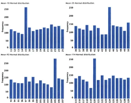
and SPS constraint consideration may differ (Wagner, 2002). Furthermore, inventory management systems in retail stores often do not account for pack sizes when suggesting orders (Interviews during store visits, 2015). Therefore, store managers tend to make "systematic corrections" to the order size that is suggested by these automated systems (van Donselaar et al., 2006). The lack of OPS consideration could lead to inefficient ordering decisions at the store level, which affects both the inventory and the space requirements in the store. Similarly, not considering SPS in or-dering decisions can lead to a mismatch between backroom capacity and the space required in it leading to inefficient utilization of the storage space.

We present some relevant empirical evidence related to OPS and SPS using data from our industry partner, which is a major US retailer and referred to as Deltaco in the thesis. A single store backroom has multiple SKUs, which have different order and storable pack sizes. For example, in Figure 2-1, we use the data available to us for 126 Deltaco stores to show the distribution of OPS for approximately 1,000 different SKUs that are ordered and carried in the stores. Figure 2-2 shows the corresponding SPS to OPS ratio for the SKUs.

In the first part of the study, we will focus on the effect of OPS alone and assume SPS and CPS to be equal to 1. In particular, we explore and quantify the specific effect of the OPS on the inventory level and resultant space requirements in the store backroom and the service level achieved. Later, we will discuss the effect of SPS on the backroom space requirements for a given amount of inventory level.

Intuitively, one would expect that when a store manager is constrained to order in integer multiples of OPS, an OPS of greater than 1 unit results in inflated inventory levels as compared to being allowed to order in single units or eaches. Therefore, traditional inventory policies are no longer accurate. To illustrate this, we examine a periodic review and order-up-to level replenishment policy to analyze the effect of pack size. This commonly used inventory policy (Silver et al., 2016) is also used by Deltaco. When OPS is greater than 1 and the store manager plans for inventory (referred to as planned inventory) without

(29)

accounting for the OPS effect (or in other words with the assumption that OPS=1) the store could end up carrying excess inventory (referred to as actual inventory).

Distribution of order pack size of different SKUs for a major US retailer 25%

I

l

OPS range I I

I

_Io

U 0 '4 0,

IM

0i

Figure 2-1: Histogram for order pack size at Deltaco

Distribution of observed SPS to OPS ratio of the SKUs

1/6 1/4

SPS/OPS ratio

1/1 other

Figure 2-2: Histogram for ratio of storable pack size to order pack size at Deltaco

This inflated inventory level can have a variety of effects on store operations. On one hand, when the demand is stochastic, the excess amount of inventory can help hedge against uncertainty and yield a lower probability of stock out. However, this benefit comes at a cost of excess storage space requirements in the store along with a larger holding cost due to

20% 15% 0 10% 5% U% 0%

I

_U, A 0 4.V bC WJ 50% 45% 40% 35% 30% 25% 20% 15% 10% 5% 0% 1/12

(30)

excess inventory on hand.

In summary, when the OPS of a SKU is greater than one, there is a trade-off between improved service level and higher space requirements, increased holding costs and increased waste in case of perishable items, with increasing

OPS

values in a constrained store space environment. For the sake of simplicity, in this chapter, we focus on exploring the improved service level and the higher space requirements. So, we first quantify the excess amount of inventory and the consequent effect on storage space needs for a single SKU, which can then be used to model for optimal order-up-to levels in a retail store facing storage space constraints while dealing with multiple SKUs, as shown in chapter 3.

The remainder of the chapter is organized as follows. In section 2.2, we quantify the effect of OPS on inventory levels for deterministic demand case. Section 2.3 presents an analytical derivation of the effect of OPS when demand is uncertain as well as discusses an approximation of this effect that provides us with a closed-form expression to determine inventory levels under an OPS constraint. Section 2.4 quantifies and discusses the effect of OPS on the probability of stock-out and the expected number of stock-out units. A part of this section also describes the implied adjustment to the planned safety stock level as a result of the OPS constraint. Section 2.5 discusses the trade-off between the excess space requirement as compared to the reduction in probability of stock-out under an OPS constraint. This is followed by discussion of the effect of SPS on the space requirements in section 2.6. Finally, the chapter presents conclusions to wrap up the discussions along with potential future work in section 2.7.

2.2 Quantifying the effect of OPS on inventory

In this section, we evaluate the effect of OPS on the inventory carried in the store when the store manager is constrained to order in multiples of the OPS instead of eaches. As noted earlier, the replenishment policy used for the analysis is a periodic review and order-up-to level or (R,S) policy. This means that for each SKU, the store manager checks the inventory position and replenishes the inventory at the store to at least an 'S' level every review period R. The degree of inflation of the inventory and the required adjustment to the expected 'S' level depends on whether the product demand is deterministic or stochastic. Additionally, the setting in which the analysis is conducted is characterized by a constant

(31)

consumption rate of the SKU, lost sales scenario and an infinite time horizon. The stores are open during daytime business hours and the orders are placed at the closing of the business, which are then delivered overnight. Deliveries, therefore, have a 0 lead-time, i.e. they are instantaneous.

We examine the effect of OPS on the ending inventory in case of deterministic demand and stochastic demand. Ending inventory is defined as the amount that is available on hand at the end of a review period and before an order is placed for the next review period. The observed effect of

OPS

on the ending inventory is then used to analytically derive the average inventory on hand and the beginning inventory during the review period .

Beginning inventory is the inventory level that is observed right after receiving delivery of the order. A limited service restaurant retailer like Deltaco sometimes processes and combines the SKUs that are ordered before they are sold. All the SKUs that are delivered to a Deltaco restaurant have to be stored in the backroom. Hence, beginning inventory level is used to determine the space requirement in the backroom of the retail store.

The beginning inventory when ordered in eaches (or when OPS=1) is expected to be equal to S. However, they take different values over multiple time periods when the stores are constrained to order in integer multiples of OPS while maintaining at least an inventory level of S at the beginning of every review period, due to the excess ending inventory.

2.2.1 Notation list

The following list defines the notations used for the derivation of the effect of OPS on beginning inventory.

" S: order-up-to level

* X,: beginning inventory for review period n. This is the inventory level before the store opens on day n and also includes the inventory that is delivered on day n " Y: ending inventory for review period n. This is the inventory level after the store is

closed for business on day n

" O,: number of order packs ordered and received at beginning of review period n "

Oen:

equivalent number of sellable units ordered and received at the beginning of

review period n

" r7,: order pack size or OPS

(32)

p

p: mean of the distribution of daily demand * R: review period for a SKU

* m: Greatest common divisor (GCD) of mean demand over review period and the order pack size, i.e. GCD of (p * R, %u). For example, GCD(110,20) = 10.

* [.]: The ceiling function of a positive number, which is also defined as the smallest integer greater than or equal to the number

2.2.2 Dynamics of the process of ordering and the resultant change in inventory levels

The process dynamics for ordering and the change in inventory levels under an

OPS

con-straint are as follows:

[---' if Yn__1 < S

1.0, otherwise (2.1)

Oen Ocn * 7o (2.2)

Xn = Yn_ 1 + Oen (2.3)

Y = max(X, - Z, 0) (2.4) Equation 2.1 states that orders can only be placed in integer multiples of OPS with the decision to have inventory at least up to the planned order-up-to level on the shelf. Equation 2.2 shows the corresponding number of sellable units given a certain amount that is ordered. Equations 2.3 and 2.4 show the relation between the beginning inventory, ending inventory and the demand observed.

2.2.3 Effect of OPS on beginning inventory in the case of deterministic demand

In the deterministic demand case, the beginning inventory when OPS = 1 is equal to the demand over the review period, denoted by p * R. Figure 2-3 shows the change in the inventory levels for a fixed review period when OPS is greater than 1. We note that with a change in the review period, the plot is simply scaled to the given review period and the observed behavior of the change in inventory level over time remains the same.

Specifically, Figure 2-3 illustrates the effect of OPS on the amount of cycle stock and the beginning inventory. The cycle stock and beginning inventory can be derived by observing the patterns in the ending inventory. The average ending inventory is a function of the demand over the review period and the order pack size of the SKU. The average cycle stock

(33)

160 140 120 X2 - 100 80 -60 40 20""" 0" 0 t Bkglmalm of PerIod 1 Figure 2-3: An example to carried. 7,,=100 units/case, X2 1 2 3 t

Emd of Time (in weeks) Perlodi

illustrate the effect of order p=80 units/week and R = 1 X4 XS y4 Ys -W 4 5

pack size on amount of inventory week. In this case m = 20.

and the average beginning inventory are given by equations 2.5 and 2.6, respectively. A few observations about the ending inventory and an analytical derivation for equations 2.5 and 2.6 are provided below.

Average cycle stock = + 770 - m

2 2

Average beginning inventory = M * R + 2 2

(2.5)

(2.6)

where m is the GCD(p * R, rq,)

* Property 1. Ending inventory value: Ending inventory in any time period is an integer

multiple of m.

" Property 2. Ending inventory range: Ending inventory takes all values from a fixed set that contains integer multiples (x) of m where x E {0, 1, 2,....(. - 1)}

" Property 3. Ending inventory cycle: The number of review periods over which the

ending inventory takes these fixed values is given by I (equal to 5 review periods in the example shown in Figure 2-3). In the last review period of this cycle, the beginning inventory is equal to demand over review period (X5 in the example shown) and hence

(34)

the amount ordered is 0. This also implies that the amount ordered repeats itself over this fixed number of review period cycles. However, the sequence of the values of ending inventory (and also the amount ordered) is not the same over this cycle.

For deterministic demand, when OPS > 1, the average beginning inventory in a review period is the sum of demand over review period and the average extra inventory carried, as derived below. To derive equation 2.6, we use the relation between beginning and ending inventory along with the properties of ending inventory observed from simulation to derive the average amount of beginning inventory in case of deterministic demand:

Xn = Yn-1

+

0

en = Yn- 1 + 77o * [S-Y-l770

The equation states that the beginning inventory in a period n is the sum of the ending inventory from the previous time period and the order quantity in n.

Properties 1, 2 and 3 of ending inventory imply that:

Y,-1 E m * {0,1, 2, . ... (- - 1)}.

The ending inventory takes all the values in the set. Since this pattern is repeated every ' review periods, the average beginning inventory during this time period is also the long run average of the beginning inventory in an infinite horizon setting. The average of beginning inventory is hence given by:

(i) * [(0 + ro * [ *) + (m+rnj*

**[ *-1)**

+ (2m + ,q * [I*R-2m1) + (( 0 - m)+

mmm mo

77,* [Jp*R-(??o-m)

1)]

70

-~~~ +*O12..-1

~ ~

(F'L-R1 + [/I*R-m] _{+ [pL*R-2mj +} _+.[p*R-(7hom)j)

m (!1 * *(1 + [M*( [~LLR + [j*R-m] + Fp*R-2

mi + +. [p*R-(hlo-m)])

770- + M *(F *R ]+rji*R _1 11*R 2 LRal

We use the following relation from (Graham et al., 1994) to obtain the value for the second part of the equation: For any positive value y and integer values of x,

T[t g + [xf1] + [x2] +... e txhy+11) = Therefore, the average beginning inventory becomes:

Backroom space allocation in retail stores