Ship Performance in Broken Ice Floes - Preliminary Numerical Simulations

Publisher’s version / Version de l'éditeur:

Technical Report, 2010-11-29

READ THESE TERMS AND CONDITIONS CAREFULLY BEFORE USING THIS WEBSITE. https://nrc-publications.canada.ca/eng/copyright

Vous avez des questions? Nous pouvons vous aider. Pour communiquer directement avec un auteur, consultez la

première page de la revue dans laquelle son article a été publié afin de trouver ses coordonnées. Si vous n’arrivez pas à les repérer, communiquez avec nous à PublicationsArchive-ArchivesPublications@nrc-cnrc.gc.ca.

Questions? Contact the NRC Publications Archive team at

PublicationsArchive-ArchivesPublications@nrc-cnrc.gc.ca. If you wish to email the authors directly, please see the first page of the publication for their contact information.

NRC Publications Archive

Archives des publications du CNRC

For the publisher’s version, please access the DOI link below./ Pour consulter la version de l’éditeur, utilisez le lien DOI ci-dessous.

https://doi.org/10.4224/17210723

Access and use of this website and the material on it are subject to the Terms and Conditions set forth at

Ship Performance in Broken Ice Floes - Preliminary Numerical

Simulations

Wang, J.; Derradji-Aouat, A.

https://publications-cnrc.canada.ca/fra/droits

L’accès à ce site Web et l’utilisation de son contenu sont assujettis aux conditions présentées dans le site LISEZ CES CONDITIONS ATTENTIVEMENT AVANT D’UTILISER CE SITE WEB.

NRC Publications Record / Notice d'Archives des publications de CNRC:

https://nrc-publications.canada.ca/eng/view/object/?id=6ffa0b09-e387-444c-b118-594a9f54695b

https://publications-cnrc.canada.ca/fra/voir/objet/?id=6ffa0b09-e387-444c-b118-594a9f54695b

DOCUMENTATION PAGE

REPORT NUMBER

TR-2010-24

NRC REPORT NUMBER DATE

November 2010

REPORT SECURITY CLASSIFICATION

Unclassified

DISTRIBUTION

Unlimited

TITLE

SHIP PERFORMANCE IN BROKEN ICE FLOES – PRELIMINARY NUMERICAL

SIMULATIONS

AUTHOR (S)

Jungyong (John) Wang and Ahmed Derradji-Aouat

CORPORATE AUTHOR (S)/PERFORMING AGENCY (S)

Institute for Ocean Technology, National Research Council, St. John’s, NL

PUBLICATION

SPONSORING AGENCY(S)

Institute for Ocean Technology, National Research Council, St. John’s, NL

IOT PROJECT NUMBER

42_2434_10

NRC FILE NUMBER KEY WORDS

Ship in ice, Numerical Calculation, LS-DYNA

PAGES

iii, 6

FIGS.

11

TABLES

3

SUMMARY

A recently developed FE (Finite Element) model for ship performance in ice is presented in

this paper. Hydrodynamic loads and ship-ice interaction loads are numerically calculated

based on the Fluid Structure Interaction (FSI) method by using commercial FE package

LS-DYNA (www.lstc.com). Actual test results from laboratory physical model scale experiments

are used to validate and benchmark the numerical simulations. One of the NRC-IOT’s

standard icebreaker models (a model for the Canadian icebreaker Terry Fox) is used in the

numerical simulations in two different concentrations (80% and 60%) of pack ice conditions.

In this paper, only broken ice conditions are numerically simulated, and therefore ice

material failure was not considered. All ice properties such as density and Young’s modulus

used are the same as those measured in the NRC-IOT ice tank. The numerical challenge is

to evaluate hydrodynamic loads on the ship hull. This is due to the fact that LS-DYNA is an

explicit FE solver and FSI value is calculated by using a penalty method. For this purpose, a

2-D wavemaker was simulated and compared with experiments. Although the hydrodynamic

loads directly acting on the ship are small compared to the ice loads, the interaction

between water and ice could be important for simulating pack ice conditions or ice floe

management. Comparisons between numerical and experimental results are shown and

main conclusions are pointed out.

ADDRESS

National Research Council

Institute for Ocean Technology

Arctic Avenue, P. O. Box 12093

St. John's, NL A1B 3T5

National Research Council Conseil national de recherches Canada Canada Institute for Ocean Institut des technologies

Technology océaniques

SHIP PERFORMANCE IN BROKEN ICE FLOES –

PRELIMINARY NUMERICAL SIMULATIONS

TR-2010-24

Jungyong (John) Wang and Ahmed Derradji-Aouat

iii

TABLE OF CONTENTS

ABSTRACT ... 1

INTRODUCTION ... 1

FLUID STSRUCTURE INTERACTION ... 1

General Governing Equations ... 2

Penalty Method ... 2

WAVEMAKER SIMULATION ... 3

SIMULATION FOR SHIP TRANSITING IN PACK ICE

(MODEL SCALE) ... 4

Floating Ice Block ... 4

Icebreaker Simulation ... 4

Bow only simulation... 5

Full ship simulation ... 5

CONCLUSION ... 6

REFERENCE ... 6

LIST OF TABLES

Table 1 Comparison between calibration data and numerical results... 4

Table 2 Simulation conditions... 4

Table 3 Full ship simulation results (average x – force)... 6

LIST OF FIGURES

Fig. 1 Physical (up) and numerical (down) wavemaker ... 3

Fig. 2 Pseudo 2-D simplified wavemaker sketch ... 3

Fig. 3 Density contour with 0.5Hz wave frequency ... 3

Fig. 4 Average pressure on the upper flap from Fluid Structure Interaction from 0.5Hz case ... 3

Fig. 5 One ice piece floating simulation ... 4

Fig. 6 Vertical displacement of ice (up) and three directional forces acting on ice (down) ... 4

Fig. 7 Bow only simulation ... 5

Fig. 8 60% (up) and 80% (down) ice concentration ... 5

Fig. 9 Contact force from bow only simulation ig. 8 60% (up) and 80% (down) ice concentration ... 5

Fig. 10 Computational domain for full ship simulation (60 % concentration) ... 5

Ship Performance in Broken Ice Floes – Preliminary Numerical Simulations

Jungyong Wang and Ahmed Derradji-Aouat

Institute for Ocean Technology, National Research Council Canada St. John’s, NL, CANADA

ABSTRACT

A recently developed FE (Finite Element) model for ship performance in ice is presented in this paper. Hydrodynamic loads and ship-ice interaction loads are numerically calculated based on the Fluid Structure Interaction (FSI) method by using commercial FE package LS-DYNA (www.lstc.com). Actual test results from laboratory physical model scale experiments are used to validate and benchmark the numerical simulations. One of the NRC-IOT’s standard icebreaker models (a model for the Canadian icebreaker Terry Fox) is used in the numerical simulations in two different concentrations (80% and 60%) of pack ice conditions. In this paper, only broken ice conditions are numerically simulated, and therefore ice material failure was not considered. All ice properties such as density and Young’s modulus used are the same as those measured in the NRC-IOT ice tank. The numerical challenge is to evaluate hydrodynamic loads on the ship hull. This is due to the fact that LS-DYNA is an explicit FE solver and FSI value is calculated by using a penalty method. For this purpose, a 2-D wavemaker was simulated and compared with experiments. Although the hydrodynamic loads directly acting on the ship are small compared to the ice loads, the interaction between water and ice could be important for simulating pack ice conditions or ice floe management. Comparisons between numerical and experimental results are shown and main conclusions are pointed out.

INTRODUCTION

A typical ship-ice interaction study was treated as structural impact analysis using decoupling from hydrodynamic loads. Combining structural and flow analysis is often prohibited due to the computational cost and also hydrodynamic loads can be small enough and negligible. Since computational capability has been significantly increased and engineering trends can be expected to focus on performance evaluation in ice-infested water, accurate modeling for both flow and structural assessment becomes more important. In the past, arctic class vessels are generally small (LPP of about 100m), but recent trends are very different; ship sizes are getting bigger, and speed is getting faster. Global warming can drive this trend even faster because Arctic ice is getting weaker and all-year round shipping area is becoming wider.

Modeling of Fluid-Structure Interaction (FSI) has been used for various circumstances in the marine engineering field. Typical examples are hydrodynamic impact on ship hull (slamming) when a ship is transiting high waves, and the sloshing problem in LNG Tanks. For the interaction between ship and ice, however, hydrodynamic loads are not the primary consideration, but they still play an important role in overall simulation and its accuracy. The reason is that both ship and ice are floating on the water and the flow field dominants the ice floe movement. For the level ice, ice failure cannot be properly simulated without appropriate buoyancy which contributes damping effect. (Wang and Derradji, 2009).

Combining structural and flow analysis enables us to assess ships and structures in ice interaction more properly. Using FSI methods, most ice interaction problems can be practically solved. For example, a drill ship in pack ice conditions, a lifeboat performance in ice covered water, ice management strategies, and so on. Like other numerical simulations, the validation process is very important and this paper shows validations using experimental data from the ice tank.

FLUID STRUCTURE INTERACTION

There are several ways to consider Fluid-Structure Interaction (FSI) problem numerically. If the structure is treated as a rigid body, then a flow solver (CFD) can integrate flow velocity field on the wetted surface area and calculate pressure or drag force (i.e. ship resistance). The disadvantage of using CFD only is having a limited capability of structure-structure interaction such as ship-ice interaction as multi deformable bodies. However, a commercial explicit FE solver, LS-DYNA, has a capability to solve the fluid flow by using an Eulerian formulation while the structure is considered as Lagrangian one. The Arbitrary Lagrangian Eulerian (ALE) method in LS-DYNA allows for the fully coupled solution of Lagrangian structures interacting with Eulerian fluids. The principle of the ALE is that Lagrangian structure is overlapped on the Eulerian computational domain. At each time step, the both Lagrangian and Eulerian calculations are independently performed and followed by remapping step (advection step) from the distorted Lagrangian mesh to Eulerian domain. The last step is interface reconstruction. Since LS-DYNA does not have a full CFD solver such

as Navier-Stokes solver, hydrodynamic calculations were estimated by penalty method. Fluid is modeled using dynamic viscosity and equations of state (EOS) with a null material model.

General Governing Equations - Continuity Equation

In fluid mechanics, continuity equation can be written as eq. (1)

0 ) (∇⋅ = +ρ v ρ dt d (1)

In the material form it can be written as eq. (2)

dV t z y x dV t z y x V V ) , ' , ' , ' ( ) , , , ( 0 0 0 0

∫

ρ =

∫

ρ using Jacobian J,

∫

− = 0 0 ) ( 0 0 V ρ ρJ dV , J ρ ρ0= (2) - Momentum Equation

Since the time rate of change of total momentum of system is the same as the vector sum of all the external force, Eq. 3 can be made.

∫

+

∫

=

∫

S V _dt V dV d dV dS b v t ρ ρ (3) where ρis the density, t is the surface traction and b is the body force per unit mass.

Using Cauchy stress tensor (

σ

), t=σij⋅n, and divergence theorem,

∫

∫

∫

∇⋅ + = V V V ij dV dt d dV dV ρb ρv σ b b v _{ρ σ ρ σ ρ} ρ = x=∇⋅ ij+ = ijj+ dt d , (4) - Energy Equation

Using total energy ( E ) which is the sum of kinetic energy and internal energy, v b E ρ ε σ ρ = ij ij+ dt d (5)

In LS-DYNA, the modified energy equation for explicit solver (eq. 6) is integrated in time and is used for equation of state evaluation and a global energy balance.

V q p V dt d ij ij −( + ) = σ ε ρ E (6) where V is the relative volume which is the determinant of Jacobian,

pis the hydrostatic pressure and q is the bulk viscosity.

Since the FEM is to solve the weak form of the momentum equation (principle of virtual work), it can be written as Eq. 7.

0 , − − = + =

_∫

_∫

_∫

_∫

S i V i i V ij ij V i dS x dV x dV x dV x xδ σ δ ρ δ δ ρ δπ b t (7) For time integration, the central-difference method is adopted in LS-DYNA, which is shown in Eq. 8.

) 2 ( 1 2 t t t t t t t −∆ − + +∆ ∆ = U U U U ) ( 2 1 t t t t t t − −∆ + +∆ ∆ = U U U (8) where ∆tis the time step size.

In order to fomulate ALE (Arbitrary Lagrangian Eulerian), two domains are considered; material (spatial) domain and reference domain. The ALE governing equations are derived for the case when the reference frame moves at an arbitrary velocity. The material velocity is u , reference frame velocity is v and their differences,

v

u− is expressed as w . The basic ALE formulation is shown in Eq. 9.

i i x v J t J ∂ ∂ = ∂ ∂ (9)

where J is the Jacobian which is the relative differential volume between two domains.

The material time derivatives in ALE is written in Eq. 10.

x f w t r ∂ ∂ − = ∂ ∂ b b (10) where r

b means that b is expressed as a function of the reference domain.

Therefore ALE equations for conservation of mass, momentum and energy are: i i i i r x w x u t ∂ ∂ − ∂ ∂ − = ∂ ∂ρ _ρ ρ j i j i j ij r i x u w b t u ∂ ∂ − + = ∂ ∂ _{σ ρ ρ} ρ ( , ) (11) j j i i j i ij r x e w u b u t e ∂ ∂ − + = ∂ ∂ _{σ ρ ρ} ρ ( _, ) Penalty Method

Penalty method was used for contact (between Lagrangians) and coupling (between Lagrangian and Eluerian) for this simulation. It is the same concept but the detailed calculation for interaction loads is somewhat different. The coupling load calculation is loosely based on the vibration problem with two masses and one spring in between, and the detailed formula is proprietary. Contact force (between Lagrangians) calculation using the penalty method is explained here. For example, when the slave contacted the master surface, the interface force is generated between the slave node and contact surface. The interface force is proportional to its penetration through the master element, and pushing back the slave node at the reverse direction of penetration in order to maintain the contact surface. The force can be calculated by Eq. 12 such as a spring.

kd

F=− (12) where k is the stiffness factor and d is the penetration distance. The stiffness factor

k

is shown in Eq. 13.

V KA p k f 2 = (13)

where p is the scale factor for the interface stiffness, K is the bulk _f modulus, A is the face area, V is the volume of the master segment. This method is suitable for wide range of fluid-structure interaction application, but the forces were always estimated and consequently oscillated. More detailed description is referred to LS-DYNA Theory manual (LS-DYNA, 2006).

WAVEMAKER SIMULATION

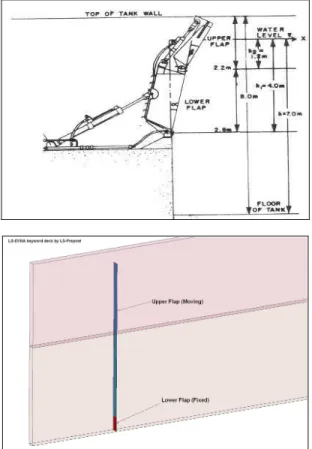
Wavemaker simulation using ALE method is presented in this section. The physical wavemaker at NRC-IOT has been installed and used for 25 years at the 200m towing basin. Calibration data of the wavemaker including wave length and wave height published by Datta and Murray (1986) was compared with the simulation results. The wavemaker has dual flaps and four different operating modes, but the present simulation showed only one mode (operating upper flap alone) to verify the capability of ALE.

Pseudo1 2D model for the wave maker in the tank was developed with full moving upper flap and only top part of fixed lower flap (See Figs. 1 and 2). At the end of the wave tank, ambient elements with pressure inflow condition (act as a non-reflecting boundary) were inserted in order to avoid any reflecting wave to disturbed newly generated wave from the wavemaker. No water and air will pass through the bottom, top and both sides.

Fig. 1 Physical (up) and numerical (down) wavemaker

1

One element thick (0.1m) wave tank model

WATER AIR Lower Flap (Fixed) Upper Flap (Moving) 1.2 m 1.4 m 20 m Ambient Element (Pressure inflow)

Fig.2 Pseudo 2-D simplified wavemaker sketch

Regular waves with different wave frequency were simulated. The wavemaker movement was determined by the time versus x-movement (horizontal displacement) curve to move the rigid upper flap. The half-stroke flap angle of 6 degree was used and the range of the wave frequency was from 0.5 to 0.7 Hz with 0.1 Hz interval. For the simulation, wave height and wave length were roughly measured based on the density plot at each wave frequency. Total number of elements is about 5000 and each simulation has a 30 second period, which takes about 2 physical hours to calculate with a 4 CPU machine. As an example, the density contour for the 0.5 Hz simulation is shown in Fig. 3. Fig. 4 shows the FSI (Fluid Structure Interaction) pressure value acting on the whole upper flap. It shows good agreement with regard to upper flap movement.

Fig. 3 Density contour with 0.5Hz wave frequency

Fig. 4 Average pressure on the upper flap from Fluid Structure Interaction from 0.5Hz case

Table 1 shows the comparison between calibration data and numerical results. Since this is a preliminary simulation with a coarse element (element size is 0.1m), the wave height (range of 0.2 m - 0.3 m) comparison is not quite feasible with regard to given element size. For the wave length, however, the magnitude is more appropriate with the element size and it shows a good agreement at higher frequency (more than 0.6 Hz). Unlike any other numerical results, these wave height and

length are measured from graphics with density contour, so that it may include certain amount of uncertainty.

Table 1. Comparison between calibration data and numerical results Wave Height (m) Wave Length (m) Hz Experiment Numerical Experiment Numerical 0.5 0.18 ~ 0.21 0.2 6.25 5.7 0.6 0.22 ~ 0.25 0.3 4.34 4.1 0.7 0.24 ~ 0.29 0.3 3.2 3.1 0.8 0.29 ~ 0.32 0.2 2.44 2.3

SIMULATION FOR SHIP TRANSITING IN PACK ICE (MODEL SCALE)

Floating Ice Block

One of the key studies in this broken ice floe (pack ice) simulation is appropriate behavior of ice pieces. Since calculation time (time step,

e

t

∆ ) is very sensitive to the element size (Eq. 13), we tried to set an optimum element size using one ice piece floating simulation.

(

_{2 2}

)

1/2 c Q Q L t e e + + = ∆ (13) where Q is a function of bulk viscosity, c is the adiabatic sound speed and L is a characteristic length (for solid, e

max e e e A v L = , v is the element e

volume, A_emaxis the area of the largest side).

For a simple test, square water tank with one ice piece was simulated. Element size of water and air is 0.1 m, while ice thickness is 0.02m. Initial condition of ice placed is shown in Fig. 5 (up). Fig.5 (down) also shows the density ISO-surface plot with half-filled element. The ice piece was held with top surface at water level for the first 2 seconds and then released without any constraint. In order to check the buoyancy force, vertical (z direction) displacement and forces at three directions were measured and showed in Fig. 6. From this set up, a thin ice piece was properly simulated with regard to z-displacement and average buoyancy force.

Fig. 5 One ice piece floating simulation

Fig. 6 Vertical displacement of ice (up) and three directional forces acting on ice (down)

Icebreaker Simulation

From the single floating ice block simulation, 0.1m of ALE element size would be appropriate for the present pack ice simulation. From the ice model tests, there is no significant submergence of ice pieces but mainly floating on the water surface. The icebreaker used in this paper is the Canadian Coast Guard Terry Fox (21.9 model scale) was tested in the ice tank with different pack ice concentrations (80% and 60% coverage). The objective of this simulation is to assess ship performance in pack ice conditions using total force comparison. Two different ice thicknesses (20 mm and 40 mm) are used. Before simulation for the full size model ship, bow only part was simulated to ensure an appropriate interaction. Table 2 shows the simulation conditions.

Table 2 Simulation conditions

Bow Only Full Ship Nominal Element Size 0.1m 0.1m Number of Elements 25,000 60,000 Domain Size 5m (L) * 3m (W) * 1.5m (H) 15m (L) * 3m (W) * 1.2 (H) Calculation Time using 4 cpus 22 min/1sec simulation time 58 min/1sec simulation time

For both cases nominal element size was about 0.1 m. For bow only simulation, 0.9 m of water depth and 0.6 m of air height were used. For full ship simulation, however, 0.9 m of water depth and 0.3 m of air height were used to reduce the domain size. Ice floe shapes are square with dimensions of 0.15 m by 0.15 m. In order to maintain the given concentration, rigid frames at both sides and the far end were used. It is noted that these rigid frames did not interact with water/air, but did

interact with ice blocks.

Bow only simulation

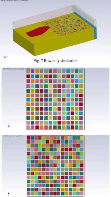
Figs. 7 and 8 show the computational domain for bow only simulation and ice concentrations, respectively. Ship and ice are modeled as rigid bodies. A force dynamometer is implemented in the ship, so that contacting forces from ice pieces are measured.

Fig. 7 Bow only simulation

Fig. 8 60% (up) and 80% (down) ice concentration

Fig. 9 shows the contact force comparison between 60 % and 80 % concentrations of the pack ice. For the simulation of 80 % concentration, ice pieces were stuck on the shoulder of the ship, which caused large load approximately between 2 and 3 seconds. Enclosed boundary may also affect the load increase at the higher concentration.

Time (Sec) L o a d (N ) 0 1 2 3 4 0 20 40 60 80 60 % 80 %

Fig. 9 Contact force from bow only simulation

Full ship simulation

Figs. 10 and 11 show the computational domains for the full ship simulation before start and during transiting ice filed, respectively.

Fig. 10 Computational domain for full ship simulation (60 % concentration)

Fig. 11 Simulation for ship transiting in pack ice (60% concentration)

From this simulation, x-force was measured and compared. Two different speeds (0.4 m/s and 0.6 m/s) and ice thicknesses (20mm and 40mm) were simulated. Table 3 shows the simulation results. Since the experiments show the range of 6 – 10 N for all these cases, 40 mm simulation results overestimate. We assumed that pack ice condition did not have much breaking or crushing phenomena but have clearing as pushing away from the ship at the water surface. For this reason, this paper modeled the ice as a rigid body and it seemed to work for thinner ice (20 mm) based on ice movements (loads are slightly overestimated). The thicker ice (40mm), however, rigid body assumption for ice is apparently not valid. Possible reasons are follows:

1. Rigid body – there is no way to consider ice deformation for energy absorption, which could more affect on thicker ice; 2. Ice regularity – thicker ice could more chance to be stuck

3. Boundary effect – it may be too close to consider proper pack ice movements;

4. Mesh dependency – it needs to be tested.

Table 3 Full ship simulation results (average x – force)

20mm, 60% concentration 40mm, 60% concentration

0.4 m/s 15 (N) 54 (N) 0.6 m/s 16 (N) 74 (N)

CONCLUSION

In this paper, Fluid-Structure Interaction (FSI) capability of a commercial explicit Finite Element Code was assessed and some applications were presented. Wavemaker simulation shows the good FSI results with regard to wave length comparison. Ice block floating simulation shows that proper buoyancy force was estimated and ice behaviors were appropriate. Using bow only and full ship, ship performance in pack ice conditions were evaluated. As the first assumption, there are no significant ice breaking, crushing and submergence of the ice and rigid body was used for the simulation. Even though ice behaves correctly, the simulation didn’t show ice load properly at high speed and high concentration. Possible reasons including rigid body mechanics, ice geometry, boundary effect and mesh dependency were addressed. This study is a preliminary study to assess FSI in FE code, and it turns quite promising feature to assess complex real scenarios such as ship, ices, and water/air altogether. As

the next step a proper ice model (deformable body) with more realistic ice geometry and proper boundary set-up will be considered in order to increase reality and accuracy.

REFERENCE

Datta, I. and Murray, J. J., 1986, “Calibration of Towing Tank Wavemaking System at the Institute for Marine Dynamics,” 21st American Towing Tank Conference, 5-7 August 1986, Washington, DC : 175- LM-HYD-12

LS-DYNA, 2006, “Theoretical Manual,” Livermore Software Technology Corporation, USA.

Wang, J. and Derradji-Aouat, A., 2009, “Implementation, Verification and Validation of the Multi-Surface Failure Envelope for Ice in Explicit FEA,” POAC09, June 9-12, Lulea, Sweden.