Publisher’s version / Version de l'éditeur:
Water Distribution Systems Analysis 2010, pp. 968-982, 2010
READ THESE TERMS AND CONDITIONS CAREFULLY BEFORE USING THIS WEBSITE. https://nrc-publications.canada.ca/eng/copyright
Vous avez des questions? Nous pouvons vous aider. Pour communiquer directement avec un auteur, consultez la
première page de la revue dans laquelle son article a été publié afin de trouver ses coordonnées. Si vous n’arrivez pas à les repérer, communiquez avec nous à PublicationsArchive-ArchivesPublications@nrc-cnrc.gc.ca.
Questions? Contact the NRC Publications Archive team at
PublicationsArchive-ArchivesPublications@nrc-cnrc.gc.ca. If you wish to email the authors directly, please see the first page of the publication for their contact information.
NRC Publications Archive
Archives des publications du CNRC
This publication could be one of several versions: author’s original, accepted manuscript or the publisher’s version. / La version de cette publication peut être l’une des suivantes : la version prépublication de l’auteur, la version acceptée du manuscrit ou la version de l’éditeur.
For the publisher’s version, please access the DOI link below./ Pour consulter la version de l’éditeur, utilisez le lien DOI ci-dessous.
https://doi.org/10.1061/41203(425)88
Access and use of this website and the material on it are subject to the Terms and Conditions set forth at
Impact of soil properties on pipe corrosion: re-examination of
traditional conventions
Kleiner, Yehuda; Rajani, Balvant; Krys, Dennis
https://publications-cnrc.canada.ca/fra/droits
L’accès à ce site Web et l’utilisation de son contenu sont assujettis aux conditions présentées dans le site LISEZ CES CONDITIONS ATTENTIVEMENT AVANT D’UTILISER CE SITE WEB.
NRC Publications Record / Notice d'Archives des publications de CNRC: https://nrc-publications.canada.ca/eng/view/object/?id=8d05c3d6-5671-406d-ad2c-80483a585a5f https://publications-cnrc.canada.ca/fra/voir/objet/?id=8d05c3d6-5671-406d-ad2c-80483a585a5f
http://www.nrc-cnrc.gc.ca/irc
I m pa c t of soil prope rt ie s on pipe c orrosion: re -e x a m ina t ion of
t ra dit iona l c onve nt ions
N R C C - 5 3 6 1 1
R a j a n i , B . B . ; K l e i n e r , Y .
S e p t e m b e r 2 0 1 0
A version of this document is published in / Une version de ce document se trouve dans:
Water Distribution System Analysis 2010 - WDSA2010, Tuscon, AZ, USA,
September 12-15, 2010, pp. 1-13
The material in this document is covered by the provisions of the Copyright Act, by Canadian laws, policies, regulations and international agreements. Such provisions serve to identify the information source and, in specific instances, to prohibit reproduction of materials without written permission. For more information visit http://laws.justice.gc.ca/en/showtdm/cs/C-42
Les renseignements dans ce document sont protégés par la Loi sur le droit d'auteur, par les lois, les politiques et les règlements du Canada et des accords internationaux. Ces dispositions permettent d'identifier la source de l'information et, dans certains cas, d'interdire la copie de documents sans permission écrite. Pour obtenir de plus amples renseignements : http://lois.justice.gc.ca/fr/showtdm/cs/C-42
Water Distribution System Analysis 2010 – WDSA2010, Tucson, AZ, USA, Sept. 12-15, 2010
IMPACT OF SOIL PROPERTIES ON PIPE CORROSION:
RE-EXAMINATION OF TRADITIONAL CONVENTIONS
Yehuda Kleiner, Balvant Rajani and Dennis Krys
National Research Council of Canada, Institute for research in ConstructionOttawa, Ontario, Canada Yehuda.Kleiner@nrc-cnrc.gc.ca
Abstract
Soil corrosivity is not a directly measurable parameter and pipe corrosion is largely a random
phenomenon. The literature is replete with methods and systems that attempts to predict soil corrosivity and resulting metallic pipe corrosion from soil properties (e.g., resistivity, pH, redox potential and others) surrounding the pipe.
This paper describes research that endeavors to gain a thorough understanding of the geometry of external corrosion pits and the factors (e.g., soil properties, appurtenances, service connections, etc.) that influence this geometry. This understanding would lead to the ultimate objective of achieving a better ability to assess the remaining life of ductile iron pipes for a given set of circumstances.
Varying lengths of ductile iron pipes were exhumed by several North American and Australian water utilities. The exhumed pipes were cut into sections, sandblasted and tagged. Soil samples extracted along the exhumed pipe were also provided. Pipe segments were scanned, using a specially developed laser scanner. Scanned data were processed using specially developed software. Statistical analyses were performed on three geometrical attributes, namely pit depth, pit area and pit volume. Various soil characteristics were investigated for their impact on the geometric properties of the corrosion pits. Preliminary findings indicate that the data not always support traditional conventions.
Keywords
Corrosion pits, soil properties, corrosion pit geometry, probability distribution
1. INTRODUCTION
The literature is replete with methods and systems that endeavor to predict metallic pipe corrosion from the properties of the soil surrounding the pipe. Soil properties that have been implicated include soil electrical resistivity, pH value, redox potential, and sulfates in the soil solution, chloride concentration, moisture conditions, shrink/swell properties and others. However, soil corrosivity is not a directly measurable parameter and corrosion is largely a random phenomenon, hence, no explicit relationships exist between these soil properties and soil corrosivity as well as between soil corrosivity and pipe deterioration rate. Virtually all the models that endeavor to propose such relationships are empirical. Some of the more practical approaches found in the literature largely based on empirical observations, some or all of the aforementioned soil properties with soil corrosivity and potential pipe deterioration. The most widely
known of these approaches is the 10-point scoring method proposed by AWWA (Appendix A of ANSI/AWWA C105/A21.5), which classifies a soil as corrosive/noncorrosive based on the weighted aggregation of 5 soil properties. The 25-point scoring method of Spickelmire (2002) is similar scheme as the AWWA 10-point method except that many other factors are included. As the 10-point method yields a binary response (corrosive/noncorrosive), some attempts have been made to fine-tune it using soft
computing techniques, e.g., Sadiq et al. (2004) and Najjaran et al. (2006).
Among the researchers who investigated the usage of statistical/probabilistic tools to characterize the properties of corrosion pits, a few are noted: Logan and Koenig (1939) proposed some practical methods for pipe sampling. Aziz (1956) was among the first to use extreme value statistics (EVS), albeit not specifically for pipes but for aluminum samples immersed in water. He proposed the double exponential (or Gumbel) distribution for the analysis corrosion pit maxima. Hay (1984) also found that the Gumbel distribution fitted corrosion pit maxima well in buried cast iron pipes. He subsequently examined, using multiple regression, the impact of soil properties on pit maxima and found that the most significant factor in predicting corrosion rate was the logarithm of the reciprocal of the linear polarization resistance (LPR), followed by total soil acidity measures in the form of extractable aluminum and extractable cations (Ca, Mg, Na) in the soil.
Sheikh et al. (1989) proposed a truncated exponential distribution as the underlying distribution for pit depth and Sheikh et al. (1990) proposed a probabilistic model to predict time to failure. Laycock et al. (1990) used the generalized extreme value statistic to analyze corrosion pit maxima and subsequently extrapolate sample data in time and space. Scarf et al. (1992) extended the work of Laycock et al. (1990) to consider the r deepest pits in a sample rather than just the single deepest pit. Katano et al. (1995) and Katano et al. (2003) found that the log-normal distribution best fitted their pit data and using regression analysis observed that the environmental factors that were found to be the most significant in determining pit depth (for a given exposure time) included soil type, pH, resistivity, redox potential and sulfate ion. Melchers (2003, 2004a, 2004b) applied multi-phase power models (as a function of time) to corrosion data collected from mild and low-alloy steel coupons subjected to “at-sea” conditions. Melchers (2005b,c) questioned the use of extreme value distribution such as Gumbel to represent the distribution of corrosion pit depth maxima and reasoned that corrosion pits form two populations, one of metastable pits (those pits that initiate but stop growing immediately or a short while after initiation) and stable pits (those pits that continue to grow).actually exist on the specimen.
Restrepo et al. (2009) applied the proportionate stratified sampling method to establish “index of
aggressiveness” (IA) of the soil, with contributors including soil moisture, pH, redox potential, soil–pipe potential , soil resistivity, and sulphide content. Caleyo et al. (2009) investigated the distributions of several soil properties along a 50-year old oil steel pipeline. They then proposed a Rossum-type multivariate power model to predict maximum pits depths as a function of soil properties and time of exposure and used the probability distributions of the soil properties to carry on a Monte-Carlo analysis to discern the distribution of corrosion pit growth. The found that the model was most sensitive to pH, pipe-to-soil potential, pipe coating type, bulk density, water content and the dissolved chloride content, in that order
The National Research Council of Canada (NRC), with funding from the Water Research Foundation (WRF – formerly known as AwwaRF – American Water Works Association Research Foundation) has undertaken a research project to investigate the long term performance of ductile iron (DI) water mains. One of the sub-objectives of this research is to gain a thorough understanding of geometry of external corrosion pits and the factors (e.g., soil properties, appurtenances, service connections, etc.) that influence this geometry. This understanding would lead to the ultimate objective of achieving a better ability to assess the remaining life of ductile iron pipes for a given set of circumstances.
Four North America and two Australian water utilities exhumed each about 300 ft (91.4 m) of DI pipes that were slated for replacement. The exhumed pipes were cut into sections, sandblasted and tagged. Soil samples extracted along the exhumed pipe were also provided. Pipe segments were scanned, using a laser scanner that was specially developed at the NRC for this purpose and scanned data processed using special software developed for this purpose. Statistical analyses were performed on three geometrical attributes, namely pit depth, pit area and pit volume. Various soil characteristics were investigated for their impact on the geometric properties of the corrosion pits. This is an on-going research and in this paper we describe the acquisition of the data and present some of preliminary results obtained so far.
2. DATA COLLECTION, CLEANSING AND PREPARATION
Of the data on exhumed DI pipe from the six water utilities, only three data sets have been processed to date. Table 5.1 provides the details on pipe sizes, length and year of installation. The water utilities were also requested to recover soil samples every 7.6 to 15.2 m (25 to 50 ft) along the exhumed pipe. These soil samples were sent to local testing laboratories to measure soil properties as suggested in AWWA
C105/A21.5-99. The ranges of soil properties obtained from these tests are given in Table 2.
Table 1. Exhumed pipes details
City (Water utility) Diameter Depth length Installation year Kansas City (Water One) 300 mm (12”) 1.07 m (3.5 ft) 91.4 m (300 ft) 1989 Louisville (Water Co.) 200 mm (8”) 1.07 m (3.5 ft) 91.4 m (300 ft) 1972 Calgary (Water Dept.) 250 mm (10”) 3.05 m (10 ft) 91.4 m (300 ft) 1969
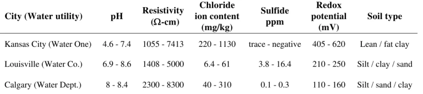
Table 2. Range of soil properties along exhumed pipes
City (Water utility) pH Resistivity
(Ω-cm) Chloride ion content (mg/kg) Sulfide ppm Redox potential (mV) Soil type
Kansas City (Water One) 4.6 - 7.4 1055 - 7413 220 - 1130 trace - negative 405 - 620 Lean / fat clay Louisville (Water Co.) 6.9 - 8.6 1408 - 5000 6.4 - 61 3.8 - 16.4 210 - 250 Silt / clay / sand Calgary (Water Dept.) 8 - 8.4 2300 - 8300 40 - 310 0.1 - 0.3 110 - 160 Silt / sand / clay
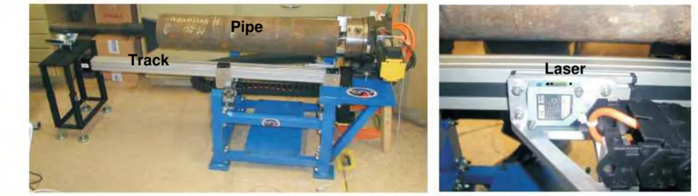
The water utilities were also asked to cut the individual pipe segments, which are typically 5.5 m or 6.1 m (18 or20 ft) long, into sections of about 1.1 m (3½ ft) long, to be scanned by a pipe laser scanner that was specially developed for this purpose (Figure 1). The water utilities were asked to tag each pipe segment sequentially as they were removed from the trench. After the pipe segments were cut into smaller sections, the exterior pipe surfaces were sandblasted to reveal 'corroded' or 'graphitized' ductile iron before carrying out the pipe scans. The contractor/sand blasters were instructed to use low nozzle velocities and avoid excessive blast times to prevent metal abrasion as well as to immediately cut back on both if “blistering” or “slivering” occurred. This resulted normally in dull light gray pipe surfaces.
Pipe Track
Laser fi d
Figure 1. Pipe Scanner (left: pipe mounted ready for scanning; right: laser finder mounted on track).
θ
ρ
x
Laser finder
Figure 2. Schematic representation of pipe scanner data.
Pipe scanning involves the back and forth movement of a laser range finder mounted on a track that is placed parallel to the longitudinal pipe axis. When the laser range finder reaches either end of the pipe, the pipe rotates a specified amount, depending on the desired scan resolution and the pipe diameter. For every
data point the scanner records the longitudinal distance x along the pipe, the rotation θ, and the distance ρ
from the laser range finder to the pipe surface, (Figure 2). The pipe scanning process terminates when θ reached 360 degrees. The scanning resolution was set to provide data points spaced at 1.5 mm grid (i,e., 1.5 mm spacing along both longitudinal and circumferential directions).
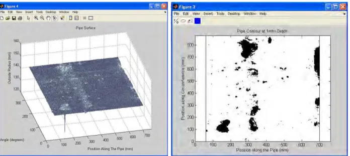
Raw data obtained from the scanner can typically suffer from a number of problems. For example, if the pipe was not perfectly aligned in the Scanner, the scan data will show a pipe surface that looks warped or bent. Also, under some conditions (oily pipe surfaces, asphaltic residue on the pipe, especially near repairs and service connections) the laser sometimes had accuracy problems reading the pipe surface, often indicating through-holes where there were none. Using software specially developed for this purpose, a six-step process was used to record the data and remove these undesired effects: (a) read in raw data and apply a raw data filter; (b) rearrange the data into a grid; (c) establish the ‘correct’ pipe surface; (d) apply 2-D grid-level filter; (e) apply 3-D grid-level filter; and (g) for statistical analysis remove unusable data. The nature of the various filters applied to the data is beyond the scope of this paper. The results of this data cleansing process can be visualized as demonstrated in Figure 3.
Figure 3: Data visualization: 3-D foldout (left) and pit contour (right).
STATISTICAL ANALYSIS OF RING POPULATIONS
Each of the exhumed pipes was virtually sliced into segments (or rings) of x length, where x = 25, 50, 100, 150, 300, 450 and 600 mm (approx. 1, 2, 4, 6, 12, 18 and 24 inch). Thus for example, an exhumed pipe of 10 m (10,000 mm) length would produce a population of 400 rings 25 mm long, or a population of 200 rings 50 mm long, and so on. This means that data for each exhumed pipe was exmainded seven different times with seven different ring populations. For each population, three pit properties were investigated, namely, the distribution of maximum pit depth in a ring, the distribution of the corroded surface area in the rings and the distribution of pit volume in the rings.
Three different types of fundamental probability distributions and three right-truncated versions of these distributions were examined as candidates to describe pit-depth population. The right-truncated versions were explored because the properties of the pit populations are (or can be) right-truncated. For example, the value of pit depth is limited by the pipe wall-thickness, which in this case would serve as the upper boundary of the truncated probability distribution. The fundamental distributions explored included Weibull (2-parameter), Gumbel (or double-exponential) and exponential. Distribution parameters were discerned using the maximum likelihood method. The chi-square test was used to ascertain ‘goodness of fit’ (in all cases there were sufficient data to warrant chi-square test).
Each ring population was fitted with six different probability distributions. Discerned distribution parameters are shown, as well as the P-value of the chi-square test. It should be remembered that the null hypothesis in the chi-square test is that the observed and modeled frequencies come from the same probability distribution. The P-value can be loosely interpreted as “what is the probability of observing such quality of fit (between observed and modeled frequencies) without these frequencies actually belonging to the same probability distribution”. Therefore, the lower the P-value the better the fit. Typically, at P-value of 0.95 (equivalent to 5% confidence level) the null hypothesis is not rejected. For the maximum pit depth distribution, among all the cases tested, the truncated Gumbel distribution was the most consistent in yielding low (often the lowest) P-values. This bodes well with theoretical expectations because it is an extreme value distribution and the population at hand is indeed truncated.
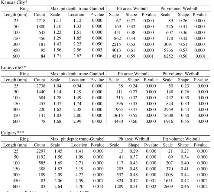
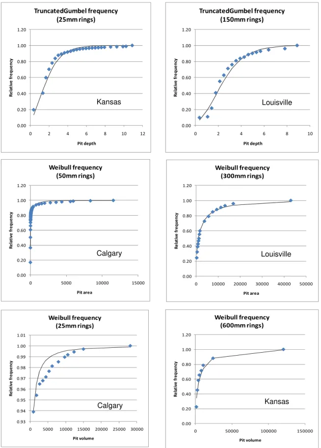
For the total pit area as well as for the total pit volume distributions, among all the cases tested, the Weibull distribution was the most consistent in yielding low (often the lowest) P-values. In most cases examined, the fundamental distribution results did not differ much from their truncated counterparts. This is expected because none of the rings in any of the cities had its entire surface covered with corrosion pits. Table 3 provides results of the analysis of maximum pit depth, pit area and pit volume in the various ring sizes from the exhumed pipes of three cities. Only those distributions that emerged as having consistently good fits are shown in Table 3. Figure 4 provides some samples to demonstrate the quality of fit.
Table 3. Statistical analysis results of pit geometries in ring populations Kansas City*
Ring Max. pit depth: trunc-Gumbel Pit area: Weibull Pit volume: Weibull Length (mm) Count Scale Location P-value Scale Shape P-value Scale Shape P-value
25 2718 1.11 1.12 0.000 67 0.27 0.000 89 0.26 0.000 50 1380 1.16 1.33 0.000 169 0.32 0.000 226 0.31 0.000 100 645 1.23 1.61 0.000 451 0.38 0.000 607 0.36 0.000 150 456 1.29 1.85 0.000 862 0.44 0.000 1178 0.42 0.000 300 181 1.43 2.23 0.050 2215 0.53 0.000 3091 0.51 0.000 450 95 1.56 2.56 0.003 4013 0.61 0.000 5766 0.57 0.000 600 84 1.71 2.62 0.006 4519 0.59 0.001 6252 0.56 0.001 Louisville**
Ring Max. pit depth: trunc-Gumbel Pit area: Weibull Pit volume: Weibull Length (mm) Count Scale Location P-value Scale Shape P-value Scale Shape P-value
25 2738 1.04 0.94 0.000 38 0.24 0.000 50 0.23 0.000 50 1440 1.14 1.19 0.000 111 0.27 0.000 148 0.26 0.000 100 684 1.28 1.49 0.000 313 0.32 0.000 432 0.30 0.000 150 455 1.37 1.74 0.000 596 0.35 0.000 844 0.33 0.000 300 220 1.62 2.38 0.000 1965 0.47 0.000 2959 0.44 0.000 450 141 1.83 2.80 0.000 3615 0.55 0.000 5608 0.50 0.000 600 78 1.68 2.99 0.003 4480 0.60 0.000 6916 0.55 0.000 Calgary***
Ring Max. pit depth: trunc-Gumbel Pit area: Weibull Pit volume: Weibull Length (mm) Count Scale Location P-value Scale Shape P-value Scale Shape P-value
25 2297 1.45 1.41 0.000 13 0.29 0.000 21 0.27 0.000 50 1192 1.56 1.99 0.000 41 0.37 0.000 69 0.34 0.000 100 585 1.69 2.71 0.000 117 0.43 0.000 207 0.40 0.000 150 388 1.87 3.19 0.000 205 0.45 0.000 370 0.41 0.000 300 189 2.09 4.22 0.000 532 0.48 0.000 1008 0.44 0.000 450 83 2.06 4.59 0.007 824 0.47 0.001 1651 0.42 0.002 600 83 2.64 5.70 0.014 1289 0.51 0.002 2609 0.46 0.002 *mean wall thickness (upper boundary) 10.89 mm
** mean wall thickness (upper boundary) 8.89 mm *** mean wall thickness (upper boundary) 8.44 mm
Figure 4. Sample distribution plots. 0.00 0.20 0.40 0.60 0.80 1.00 1.20 0 2 Re la tiv e fr e que nc y Pit de TruncatedGumbel frequency (25mm rings) 4 6 8 10 12 pth 0.00 0.20 0.40 0 2 4 6 8 Re l Pit depth 0.60 0.80 1.00 1.20 10 a tiv e fr e que nc y TruncatedGumbel frequency (150mm rings) 0.00 0.20 0.40 0.60 0.80 1.00 1.20 0 5000 Re la ti v e fr e q u e n cy Pit ar Weibull freque (50mm rin 10000 15000 ea ncy gs) 0.00 0.20 0.40 0.60 0.80 1.00 1.20 0 10000 20000 30000 40000 50000 Re la ti ve fr e q u e n cy Pit area Weibull frequency (300mm rings) Calgary Louisville 0.93 0.94 0.95 0.96 0.97 0.98 0.99 1.00 1.01 0 5000 10000 15000 20000 25000 30000 Re la ti v e fr e q u e nc y Pit volume Weibull frequ (25mm ring ency s) 0.00 0 50000 100000 150000 Pit volume 0.20 0.40 0.60 0.80 1.00 1.20 Re la ti ve fr e que nc y Weibull frequency (600mm rings) Kansas Louisville Kansas Calgary
STATISTICAL ANALYSIS OF THE IMPACT OF SOIL PROPERTIES
Based on the results detailed in the previous section, regarding the probability distributions that were found to fit well the statistical properties of maximum pit depth, pit surface area and pit volume in ring population, the following models were examined to evaluate the impact of soil properties on these statistical properties. The probability distribution of maximum pit depth in rings was assumed to follow a multi-covariate truncated Gumbel distribution, where the location parameter λ is a function of soil properties, as follows:
)
exp(
)
(
)]
)
(
exp(
exp[
1
)]
)
(
exp(
exp[(
)
(
0
;
)]
)
(
exp(
)
(
exp[
)
(
1βz
=
−
−
−
=
−
−
−
=
⎪⎩
⎪
⎨
⎧
>
≤
−
−
−
−
=
−s
s
x
K
s
x
K
x
F
x
x
x
x
s
x
s
x
K
x
f
o o oλ
α
λ
α
λ
α
λ
α
λ
α
(1)where xo is the upper bound of the truncated distribution, α is the scale parameter, λ(s) is the location
parameter, which is a function of soil properties s, z is a row vector of soil properties (e.g., soil resistivity,
redox potential, etc.) and β is a column vector of soil property coefficients to be discerned by the maximum
likelihood method.
The probability distribution of corroded surface area in rings as well as for corrosion pit volume in rings was assumed to follow a multi-covariate Weibull distribution, where the scale parameter α is a function of soil properties, as follows:
) exp( ) ( ] ) ) ( ( exp[ 1 ) ( ] ) ) ( ( exp[ ) ) ( ( ) ( ) ( 1 βz = − − = − = − s s x x F s x s x s x f
α
α
α
α
α
β
β β β (2)where, β is the shape parameter, α(s) is the scale parameter, which is a function of soil properties, z is a row
vector of soil properties and β is a column vector of soil property coefficients to be discerned by the
maximum likelihood method.
The essence of analyzing the impact of soil properties on corrosion pits is to determine whether, and by how much do soil property data, through multi-covariate probability distributions, improve the ability to predict (or ‘explain’) observed variations in pit properties (maximum pit depth, pit area, pit volume) beyond the single-variate probability distributions that were fitted to these properties as described in the previous section. The determination whether an additional covariate(s) actually improves the predictive ability of a model in a statistically significant manner is done using the likelihood ratio test (e.g., Ansel and Phillips, 1994),
)] ( ) ( [ 2 ) ( ) ( ln
2 MLL reduced model MLL fullmodel model full ML model reduced ML LR=− =− − ()
where ML = maximum likelihood and MLL = maximum log-likelihood. If the full model is reduced by a single covariate then LR would be asymptotically chi-square distributed with one degree of freedom. At a confidence level of (1 - α =; and α = 0.05) 95%, consequently,
if [MLL(full model) - MLL(reduced model)] > 1.92 then the null hypothesis is rejected (at 95% confidence) and the coefficient is not zero, meaning that the covariate is significant. The notion of P-value can also be used to express the confidence level at which the null hypothesis would be rejected, given a certain LR: P-value(LR, df) = (read: “the inverse of the chi-square distribution, given an LR value and degrees of freedom”). Hence, the P-value(3.84, 1) = 0.05. It is clear that the lower the P-value, the higher the confidence that the null hypothesis can be rejected, which means that the higher the confidence that the tested covariate is statistically significant.
)]
84
.
3
2 1≅
χ
, ( [ 2 LR df inverseχ
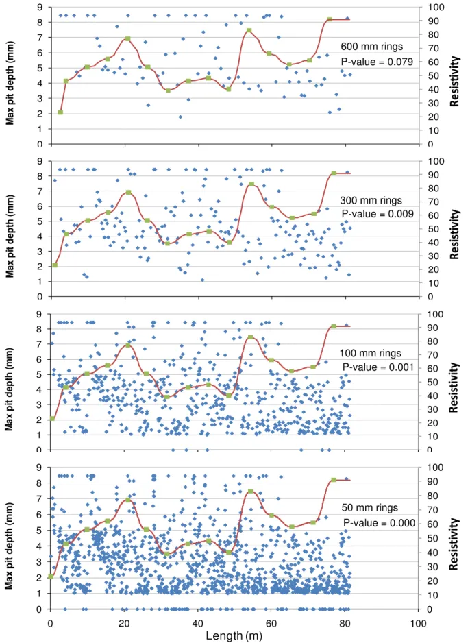
As examples Figure 5 illustrates the relationships between maximum pit depth and soil resistivity for various ring length populations in Calgary. The small dots represent maximum pit depth in each ring (left axis) and the curve represents soil resistivity measure along the pipe (the markers on the curve are actual measured values in the soil samples and the curve represents interpolated (quadratic interpolation) values. It can be seen that such a relationship is not visually apparent, and a statistical analysis is indeed required to investigate to possibility and nature of such relationship.
Soil properties considered for the Calgary analysis included soil resistivity, redox potential, chloride and sodium concentration, percent fines and soil pH. In Kansas City the same soil properties were considered except that sulphide concentration was available instead of sodium. Each of these properties was considered in two ways, absolute values and rate of change (derivative) values, where rate of change value is calculated between two adjacent soil sample locations as the difference in the soil property values divided by the distance (m) between these two points. Consequently, the analyses considered 12 soil property covariates. In addition, the distance of a ring (m) from an appurtenance was considered as well, for a total of 13 covariates.
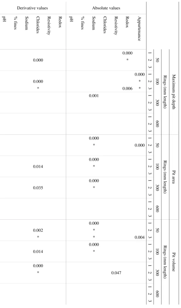
Tables 4 and 5 provide the results of soil property/corrosion pit relationship analysis in Calgary and Kansas City data, respectively. Equation 1 was used to model soil properties impact on maximum pit depths and equation 2 was used to model soil properties impact on pit area and pit volume. The likelihood ratio (LR) test was used to determine the statistical significance of these covariates. An exhaustive examination requires the LR computation of all combinations of covariates (i.e., each covariate on its own (single) – 13
cases; all possible combinations of two covariates (pair) - ܥଶଵଷ= 78 cases; all possible combinations of three
covariates (triplet) - ܥଷଵଷ = 286 cases and so forth) totaling many thousands of cases, applied to three
corrosion pit properties (maximum depth, area and volume), each with 4 possible ring lengths (50, 100, 300 and 600 mm). However, careful observation can often reduce the number of combinations requiring examination to a manageable number of a few hundred (for each of the exhumed pipes from the respective cities). A few comments, explanation and observations are warranted:
• Tables 4 and 5 show P-values. P-value of 0.05 or smaller implies that the covariate(s) is (are)
statistically significant at the 5% level. P-value of 0.01 or smaller implies that the covariate(s) is (are) statistically significant at the 1% level. The smaller the P-value the higher the statistical significance of the covariate(s). The P-values in both tables are rounded off to 3 decimal places. Only those that are significant at the 5% level (i.e., P-value ≤ 0.05) are presented.
• Three columns, 1, 2 and 3 are provided for each ring length. Column 1 shows the P-value for the single most statistically significant covariate. Column 2 shows the P-value for the most statistically significant pair of covariates and column 3 shows the P-value for the most statistically significant triplet.
Figure 5 Impact of soil resistivity on maximum pit depth (various ring lengths) in Calgary data. 0 10 20 30 40 50 60 70 80 0 1 2 3 4 5 6 7 0 20 40 60 80 100 M a x pi t de pt h ( m m ) Length (m)
R
e
si
st
iv
it
y
90 100 8 9 600 mm rings 0 10 20 30 40 50 60 70 80 90 100 0 1 2 3 4 5 6 7 8 9 0 20 40 60 80 100 M a x pi t de pt h ( m m ) Length (m)R
e
sistiv
it
y
0 10 20 30 40 50 60 70 80 90 100 0 1 2 3 4 5 6 7 8 9 0 20 40 60 80 100 M a x pi t de pt h ( m m ) Length (m)R
e
sis
tiv
it
y
0 10 20 30 40 50 60 70 80 90 100 0 1 2 3 4 5 6 7 8 9 0 20 40 60 80 100 M a x pi t de p th ( m m ) Length (m)R
e
si
st
iv
it
y
300 mm rings 100 mm rings 50 mm rings P-value = 0.079 P-value = 0.009 P-value = 0.001 P-value = 0.000
Table 4
. Calgary
Data:
P-values of various covariates in various s
cen
arios (only P-values smaller or equal to 0.0
5 are shown) M axi m u m pi t dept h Pi t area Pi t vol um e Rin g s (mm len g th) Rin g s (mm len g th) Rin g s (mm len g th) 5 0 1 00 3 00 6 00 5 0 1 00 3 00 6 00 5 0 1 00 3 00 6 00 1 2 3 1 2 3 1 2 3 1 2 3 1 2 3 1 2 3 1 2 3 1 2 3 1 2 3 1 2 3 1 2 3 1 2 3 Absolute values Appurte n ance 0.000 * * 0.000 0.004 Red ox 0.000 * 0.006 Resistiv ity 0.047 Ch lo ri d es So di um 0.001 0.000 * 0.000 * 0.000 * 0.000 * * 0.000 * % fine s pH Derivative values Red ox Resistiv ity Ch lo ri d es 0.000 0.000 * 0.014 0.035 0.002 * 0.014 0.000 * So di um % fine s pH
Maxim u m pit depth Pit area Pit volum e Rings (mm length) Rings (mm length) Rings (mm length) 50 100 300 600 50 100 300 600 50 100 300 600 1 2 3 1 2 3 12 31 2 312 312 3123 123 231 31 2 312 12 3 Absolute values Appurtenance 0.000 0.000 0.004 0.001 Redox 0.000 * 0.000 * 0.000 * 0.000 0.000 * 0.000 0.000 Resistivity Chlorides Sulphi des % fin es 0.000 * 0.000 * 0.000 * 0.000 * 0.000 * 0.000 0.000 * 0.000 0.000 pH 0.000 * 0.000 * 0.003 0.000 Derivative values Redox Resistivity Chlorides Sulphi des 0.000 0.000 0.000 * 0.000 0.000 0.000 0.025 0.004 0.037 0.002 0.000 0.000 0.000 * 0.001 % fin es pH Table 5 . Kansas City Data : P-values of
various covariates in various
scenarios ( only P-values s m aller or eq
• If generic covariate A is the single most statistically significant covariate and generic covariates A and B are the most statistically significant pair of covariates, then A’s P-value is provided in column 1, and in column 2 covariate A is represented by an asterisk. Covariate B will have a P-value in column 2, indicating its marginal contribution to the LR of the covariate pair A and B is beyond the contribution of covariate A alone. The same logic is extended to the case of three covariates.
• If covariate A is the single most statistically significant covariate and covariates B and C are the most statistically significant pair of covariates, then A’s P-value is provided in column 1, and the P-value of covariates B and C is provided in column 2. This latter P-value indicates the contribution to the LR of the covariate pair of B and C beyond the baseline, i.e., beyond the maximum likelihood value of the model with no covariates (where the LR is computed with two degrees of freedom). The same logic is extended to the case with three covariates.
• In all cases examined, except one, the marginal contribution to LR of more than three covariates was insignificant. Three columns were therefore deemed sufficient in the tables.
• In Calgary:
o Soil sodium concentration in appears to be the most consistently significant. It emerged as the
single most significant covariate in 6 out of 9 cases shown in Table 4. Out of these 6 cases, it also emerged 5 times as one of the two covariates in the most significant pair, and 1 time as one of the three covariates in the most significant triplet. Unfortunately, Calgary was the only utility that measured sodium concentration in soil samples, therefore this relatively high significance of sodium could not be compared to analyses of other cities.
o The derivative of chloride concentration also showed consistent significance. In 1 of 9 cases, it was
the single most significant covariate. In 6 out of 9 cases, it was one of the two covariates in the most significant pair. In 3 out of 9 cases, it was one of the three covariates in the most significant.
o Proximity to appurtenance emerged as somewhat significant covariate. In 1 of 9 cases, it was the
single most significant covariate. In 2 out of 9 cases, proximity to appurtenance was one of the two covariates in the most significant pair. In 2 of 9 cases, proximity to appurtenance was one of the three covariates in the most significant triplet.
o Redox potential was significant in 2 cases and resistivity in one case.
• In Kansas City:
o The derivative of sulphide concentration appears to be the most consistently significant covariate.
It emerged as the single most significant covariate in all of the 12 cases shown in Table 5. It also emerged 2 times as one of the two covariates in the most significant pair, and 2 times as one of the three covariates in the most significant triplet.
o % fines emerged 9 times out of 12 cases as one of the two covariates in the most significant pair,
o Redox potential emerged 7 times out of 12 cases as one of the two covariates in the most significant pair, and 4 times as one of the three covariates in the most significant triplet.
o pH emerged 2 times out of 12 cases as one of the two covariates in the most significant pair, and 4
times as one of the three covariates in the most significant triplet.
• It interesting to note that soil resistivity, which in the literature is often considered as the single most significant factor in pipe corrosion, showed no significance in either city.
• Another point of interest is that there is almost no overlap between the two datasets from Calgary and Kansas City with respect to the soil properties that emerged as significant covariates.
CONCLUDING COMMENTS
The methodology presented in this paper differs from others reported on in the literature in that it samples corrosion geometry in a population of equal rings rather than integral corrosion pits. Also, while pit depth or pit depth maxima were investigated in most other reports, here corrosion area and volume were investigated as well. It appears that while the truncated Gumbel (or double exponential or type I extreme value) distribution was well suited to model the histograms of pit depth maxima, the Weibull distribution was appropriate for pit area and volume, in all cities, regardless of ring length.
Examination of the impact of soil properties on corrosion pit geometries was carried out so far for two cities only. In both cities a few soil properties emerged as consistent contributors to the observed corrosion (as is reflected in their ability to increase the log likelihood of the model), but different soil properties had different contributions in Calgary and in Kansas City. This may be attributed in part to the fact that while Calgary measured sodium, Kansas City measured sulphide concentration, and both emerged as significant in the respective cities. Another explanation might be that the same soil properties impact corrosion differently in different local conditions.
It should be noted that this type of analysis investigates strictly the cases where covariates are assumed to be statistically independent. It is possible that covariate interdependencies also play a role in the impact on corrosion, which will be investigated in the future.
ACKNOWLEDGEMENT
This research project was co-sponsored by the Water Research Foundation (WRF – formerly known as the American water Works Association Research Foundation – AwwaRF), the NRC and water utilities from the United States and Canada.
.References
Ansell, J.I., and M.J. Phillips, (1994). “Practical methods for reliability data analysis” Oxford University Press, Oxford, UK.
Aziz, P.M. (1956). “Application of the statisticall theory of extreme values to the analysis of maximum pit depth data for aluminum”, Corrosion 12 (1956), pp. 495t-506t.
depth and rate in underground pipelines: A Monte Carlo study Corrosion Science 51. p. 1925–1934. Hay, L., (1984). The influence of soil properties on the performance of underground pipelines. M.Sc. thesis, Dept Soil Science, University of Sydney.
Katano, Y., Miyata, K., Shimizu, H. and Isogai, T. (1995). Examination of statistical models for pitting on underground pipes and data analysis. Proceedings of the International Symposium on plant aging and life prediction of corrodible structures, May 15-18, Sapporo, Japan..
Katano, Y., Miyata, K., Shimizu, H. and Isogai, T. (2003). Predictive model for pit growth on underground pipes. Corrosion Vol. 59, No. 2.
Laycock, P. J., R.A. Cottis, and P. A. Scarf (1990). Extrapolation of extreme pit depths in space and time. Journal of the Electrochemical Society, 137(1), pp. 64-69.
Logan, K, and Koenig, A.E. (1939). Methods of inspection of pipelines. Journal of the American Water Works Association. Vol. 31, No. 1451.
Melchers, R.E. (2003). Modeling of marine immersion corrosion for mild and low alloy steels-Part 1: phenomenological model. Corrosion (NACE), 59(4), p. 319–334.
Melchers, R.E. (2004a). Pitting corrosion of mild steel in marine immersion environment - 1:maximum pit depth, Corrosion (NACE) 60(9) 824-836.
Melchers, R.E. (2004b). Pitting corrosion of mild steel in marine immersion environment-2: variability of maximum pit depth. Corrosion (NACE), 60(10), p. 937–944.
Melchers, R.E. (2005a). Statistical characterization of pitting corrosion – 1: Data analysis, Corrosion (NACE), 61(7), p. 655-664.
Melchers, RE (2005b) Statistical characterization of pitting corrosion – 2: Probabilistic modelling for maximum pit depth, Corrosion (NACE) 61(8), p. 766-777.
Melchers, RE (2005c). Representation of uncertainty in maximum depth of marine corrosion pits. Elsevier Structural Safety, 27 pp. 322-334.
Najjaran, H., Sadiq, R., and Rajani, B. (2006). "Fuzzy Expert System to Assess Corrosivity of Cast/Ductile Iron Pipes fromBackfill Properties." Computer Aided Civil and Infrastructure Engineering, 21(1), 67-77. Restrepo, A., Delgado, J. and Echeverría, F. 2009. Evaluation of current condition and lifespan of drinking water pipelines, Journal of Failure Analysis and Prevention. 9: 541–548.
Sadiq, R., Rajani, B., and Kleiner, Y. (2004). "Fuzzy-Based Method to Evaluate Soil Corrosivity for Prediction of WaterMain Deterioration." Journal of Infrastructure Systems, 10(4), 149-156.
Scarf, P. A, R.A. Cottis, and P. J. Laycock. (1992). Extrapolation of extreme pit depths in space and time using the r deepest pit depths. Journal of the Electrochemical Society, 139(9), pp. 2621-2627.
Sheikh, A.K., Boah, J.K. and Jounas, M. (1989). Truncated extreme value model fro pipeline reliability. Reliability Engineering and System safety 25(1), pp. 1-14.
Sheikh, A.K., Boah, J.K. and Hansen, D.A. (1990). Statistical modelling of pitting corrosion and pipeline reliability. Corrosion-NACE, 46(3), pp. 190–197.
Spickelmire, B. (2002). "Corrosion Consideration for Ductile Iron Pipe." Materials Performance, 41, 16-23.