Automated open circuit scuba diver detection with low cost passive sonar and machine learning

(1)

Automated Open Circuit Scuba Diver Detection with Low Cost Passive

Sonar and Machine Learning

by

Lieutenant Commander Andrew M. Cole, United States Navy

B.S., United States Naval Academy, 2006

Submitted to the Joint Program in Applied Ocean Science & in partial fulfillment of the requirements for the degree of

Master of Science in Mechanical Engineering

at the

MASSACHUSETTS INSTITUTE OF TECHNOLOGY

and the

WOODS HOLE OCEANOGRAPHIC INSTITUTION

June 2019

The author hereby grants to MIT and WHOI permission to reproduce and to distribute publicly paper and electronic copies of this thesis document in whole or in part in any medium now known or hereafter created.

Author . . .

Joint Program in Applied Ocean Science & Engineering Massachusetts Institute of Technology & Woods Hole Oceanographic Institution May 10, 2019

Certified by . . .

Carl L. Kaiser Program Manager Woods Hole Oceanographic Institution Thesis Supervisor

Certified by . . .

Andone C. Lavery Senior Scientist Woods Hole Oceanographic Institution Thesis Supervisor

Certified by . . .

Henrik Schmidt Professor Massachusetts Institute of Technology Mechanical Engineering Faculty Reader

Accepted by . . .

Nicolas Hadjiconstantinou Chair, Mechanical Engineering Committee for Graduate Students Massachusetts Institute of Technology

Accepted by . . .

David Ralston Chair, Joint Committee for Applied Ocean Science and Engineering Massachusetts Institute of Technology Woods Hole Oceanographic Institution

(2)

(3)

Automated Open Circuit Diver Detection with Low Cost Passive Sonar and Machine Learning

by

Lieutenant Commander Andrew M. Cole, USN

Submitted to the Joint Program in Applied Ocean Science & Engineering Massachusetts Institute of Technology

& Woods Hole Oceanographic Institution on May 10, 2019, in partial fulfillment of the

requirements for the degree of

Master of Science in Mechanical Engineering

Abstract

This thesis evaluates automated open-circuit scuba diver detection using low-cost passive sonar and machine learning. Previous automated passive sonar scuba diver detection systems required matching the frequency of diver breathing transients to that of an assumed diver breathing frequency. Earlier work required prior knowledge of both the number of divers and their breathing rate. Here an image processing approach is used for automated diver detection by implementing a deep convolutional neural network. Image processing was chosen because it is a proven method for sonar classification by trained human operators. The system described here is able to detect a scuba diver from a single acoustic emission from the diver. Twenty dives were conducted in support of this work at the WHOI pier from October 2018 to February 2019. The system, when compared to a trained human operator, correctly classified approximately 93% of the data. When sequential processing techniques were applied, system accuracy rose to 97%. This demonstrated that a combination of low-cost, passive sonar and a properly tuned convolutional neural network can detect divers in a noisy environment to a range of at least 12.49 m (50 feet).

Thesis Supervisor: Carl Kaiser Title: Program Manager

Woods Hole Oceanographic Institution Thesis Supervisor: Andone Lavery Title: Senior Scientist

(4)

(5)

Acknowledgments

This research was funded by the U.S. Navy’s Civilian Institution Program with the

MIT/WHOI Joint Program. The Woods Hole Oceanographic Institution provided resources for the scuba diving conducted during the course of this thesis. I am incredibly grateful to the U.S. Navy Submarine Force for providing the opportunity to study at these two world class institutions and work closely with very talented people.

Thank you to Dr. Carl Kaiser, my primary research advisor, for his mentorship and guidance throughout my time in the Joint Program. With his busy and demanding schedule, he made my research and development a top priority. Additionally Dr. Kaiser ensured that my professional development included more than my research topic. This included visiting several Navy facilities, gaining a better understanding of the synergy between academia and the department of defense, and conducting experiments with autonomous undersea vehicles. He also enabled me to sail on a research ship in support of the AUV Sentry team. This was a unique opportunity that I will never forget.

Thank you to Mr. Edward O’Brien, the WHOI Dive Operations Manager. Without his assistance and support this research would not have been possible. Mr. O’Brien spent countless hours both improving my diving skills and conducting this experiment. The bulk of this research was conducted during winter in Massachusetts with near freezing water and limited visibility. Mr. O’Brien braved these conditions with me to conduct my experiment. I am truly grateful for his support.

Thank you to Dr. Andone Lavery, my co-advisor, for her support and guidance during my time in the MIT/WHOI Joint Program. Her direction was instrumental at reorienting me to academia and ensuring I was set up for success. Dr. Lavery’s devotion to the success of all students in the Applied Ocean Sciences and Engineering department of the MIT/WHOI Joint program and her service as the Applied Ocean Physics department education coordi-nator are very commendable.

Thank you to Professor Henrik Schmidt, my academic advisor, for his support and guid-ance during my time in the MIT/WHOI Joint Program. Professor Schmidt’s counsel enabled my success at MIT. He goes out of his way to help all Navy students in the MIT/WHOI Joint program and much of our success is owed to him. Additionally his instruction in autonomous vehicles and acoustics were both enjoyable and enlightening.

(6)

(7)

List of Figures

1-1 Four Second Spectrogram Containing a Diver Transient. . . 18

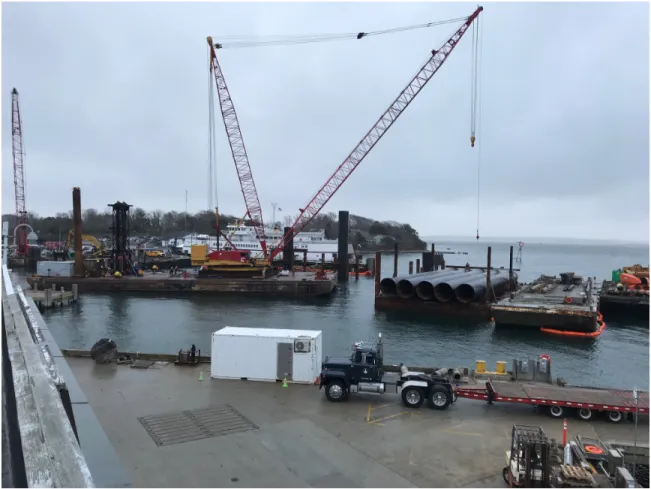
1-2 Construction at Martha’s Vineyard Ferry Terminal, 18 January 2019. . . 20

2-1 Categories of Machine Learning. . . 28

2-2 Basic Deep Convolutional Neural Network. . . 29

3-1 Overall Machine Learning Work Flow. . . 34

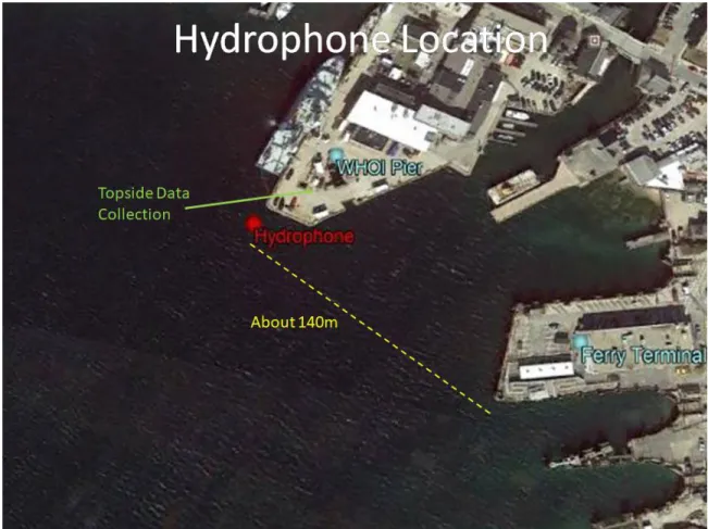
3-2 Location of Hydrophone used in the Experiment. . . 35

3-3 Spectrogram from 1013 on 19 October 2018. . . 39

3-4 Combination of Multiple Spectrograms for Data Labeling. . . 40

3-5 Diver Signature at 9.14 m (30 Feet) on 4 Different Days. . . 41

3-6 Diver Signature as a Function of Range with Low Background Noise. . . 42

3-7 Diver Signature as a Function of Range with Moderate Background Noise. . . 43

3-8 Diver Signature 1001 18 December 2018 at a range of 3.04 m (10 Feet). . . 45

3-9 Examples of Spectrograms in Machine Learning Format. . . 46

3-10 Spectrogram with Divers Only Detectable above 15 kHz. . . 48

3-11 Machine Learning Block Diagram. . . 48

3-12 Python Package Inter-Dependencies. . . 51

3-13 Block Diagram of the Deep Convolutional Neural Network Used. . . 54

3-14 Model Tuning Flow Chart. . . 55

3-15 Tuning Learning Rate: Single Frequency Model. . . 57

3-16 Training Loss and Accuracy During Training: Single Frequency Model. . . 58

3-17 Tuning Regularization Constant: Single Frequency Model. . . 60

3-18 Tuning Learning Rate: Dual Frequency Model. . . 61

(12)

3-20 Markov Chain Model for Sequential Data Processing. . . 64

3-21 Markov Chain Transition Probability Matrix. . . 65

3-22 Markov Chain Model for Low Confidence Diver Detection. . . 67

3-23 Markov Chain Model for High Confidence Diver Detection. . . 68

3-24 Spectrograms of Divers at a Range of 1.5 m to 9.14 m (30 Feet). . . 69

3-25 Diver Cross Correlation Over 10 Minutes. . . 70

3-26 Cross Correlation with Divers Range Less Than 1.5 m. . . 71

3-27 Cross Correlation with Divers Range of 3.05 m (10 Feet). . . 72

3-28 Cross Correlation with Divers Range of 12.19 m (40 Feet). . . 72

3-29 Cross Correlation on 19 October 2018 Dive. . . 73

3-30 Cross Correlation During Construction. . . 73

3-31 Cross Correlation in Presence of Broadband Transients. . . 74

3-32 Cross Correlation with Pile Driving at the Martha’s Vineyard Ferry Terminal. 75 3-33 Propagation Paths Evaluated . . . 77

3-34 Measured Vs Predicted Acoustic Pressure. . . 80

4-1 Model Generation and Independent Validation Data. . . 82

4-2 Single Frequency Model Combined Confusion Matrix for 19 December 2018 -9 January 201-9 Dives. . . 84

4-3 Dual Frequency Model Combined Confusion Matrix for 30 January - 27 Febru-ary 2019 Dives. . . 85

4-4 Dual Frequency Model Confusion Matrix for Validation Data. . . 87

4-5 Diver Detection Through Noise 1. . . 88

4-8 Construction and Tug Boat at Marta’s Vineyard Ferry Terminal 18 January 2019. . . 90

4-9 Sequential Data Processing, Divers not Present, 30 January 2019. . . 93

4-10 Sequential Data Processing, Divers Present, 30 January 2019. . . 93

4-11 Sequential Data Processing, Divers not Present, 06 February 2019. . . 94

4-12 Sequential Data Processing, Divers Present, 06 February 2019. . . 95

(13)

4-15 Spectrograms Producing False Positives Examples. . . 97

4-16 Sequential Data Processing, Divers not Present, 27 February 2019. . . 99

5-1 Diver Detection Quality as a Function of Range and Background Noise. . . . 108

(14)

(15)

List of Tables

2.1 Reported Diver Breathing Frequencies. . . 25

2.2 Reported Maximum Diver Detection Range. . . 25

2.3 Frequency Band for Diver Detection. . . 25

2.4 Diver Detection Testing Locations. . . 26

3.1 Hydrophone Recording Settings. . . 37

3.2 Spectrogram Parameters. . . 39

3.3 Hyperparameters Adjusted During Model Tuning. . . 56

3.4 Tuning Learning Rate: Single Frequency Model. . . 57

3.5 Baseline Data Augmentation Scheme. . . 59

3.6 Tuning Regularization Constant and Dropout: Single Frequency Model. . . . 60

3.7 Tuning Learning Rate: Dual Frequency Model. . . 62

3.8 Tuning Regularization Constant: Dual Frequency Model. . . 62

3.9 Model Performance on Testing Data: Dual Frequency Model. . . 63

3.10 Final Dual Frequency Model Hyperparameters. . . 63

3.11 Acoustic Arrival Path Model Final Parameters. . . 79

4.1 Single Frequency Model Performance on New Data. . . 83

4.2 Dual Frequency Model Performance on New Data. . . 85

4.3 Dual Frequency Model Performance on Validation Data. . . 86

4.4 Diver Detection Prediction as a Function of Markov State and Confidence Level. . . 91

4.5 Acoustic Model Error as a Function of Arrival Paths. . . 100

4.6 Predicted Acoustic Pressure as a Function of Diver Range and Number of Arrival Paths. . . 100

(16)

4.7 Predicted Acoustic Pressure for Various Arrival Paths. . . 102

A.1 Summary of Data Collected. . . 113 A.2 Dive Information. . . 114

(17)

Chapter 1

Introduction

1.1 Motivation

Remote detection of scuba divers is important for several reasons include monitoring the frequency of divers at recreational dive sites, identifying the presence of divers at locations where diving is forbidden (e.g. environmentally protected areas, cultural heritage sites such as shipwrecks or underwater archaeology), or preventing diver interference with aquaculture or other critical infrastructure [18][45][31]. To date, diver detection has been conducted primarily using sonar as opposed to other generally shorter range methods such as optical systems or monitoring the surface of the water for the presence of bubbles.

Either active or passive sonar can be used for scuba diver detection. Active sonar can detect divers under a wide range of conditions and has a better chance of detecting closed-circuit divers [13]. The down side to active sonar is that it requires substantial power, is expensive, and has the potential to disturb marine life [31]. Less research has been conducted on diver detection using passive sonar; however, passive sonar has the potential to be low cost, require minimal power, and it does not disturb the surrounding environment [18].

There are two main categories of divers, open-circuit and closed-circuit (rebreather) scuba divers. The need to detect closed-circuit divers is largely a military problem with a high penalty for missed detections. Active sonar is likely a better choice for closed-circuit diver detection, as the noise emitted by closed-circuit divers is generally low and cost and power are less likely of concern, as most closed circuit diver detection is military. Open-circuit scuba divers are more common than closed-Open-circuit scuba divers for civilian diving applications and generally have a louder presence in the water making them more suitable

(18)

Figure 1-1: Four Second Spectrogram Containing a Diver Transient.

for passive sonar detection. This thesis focuses on the passive acoustic detection of open-circuit scuba divers. Specifically, this thesis will show that machine learning can be used along with low-cost passive acoustic systems to detect divers even, in a noisy environment. The acoustic signature of divers is neither true narrowband, nor true broadband, making diver detection via passive sonar a non-trivial problem. If the diver signature was defined by a few discrete frequencies, detection would be accomplished using traditional automated means of identifying the presence of those frequencies. Conversely, if the diver signature was only broadband it would be indistinguishable from other broadband transients of the same duration. In this case, detection would require the method explored and is discussed in section 2.1. Instead, the diver signature is broadband with varying amplitudes across the frequency spectrum. The amplitudes and frequency bands are dependent both on the diver’s equipment and operating depth [15][33]. Figure 1-1 shows a four second spectrogram containing a diver transient. Frequency is on the X axis and time is on the Y axis. Here machine learning algorithms are used to automate proven sonar interpretation techniques for such problems. The ability to automatically detect this type of signature using passive sonar likely has other uses that are outside the scope of this thesis.

Diver detection with passive sonar may have limitations when conducted in a real world port environment. This work is discussed in section 2.1. The common thread in previous work is it attempted to use traditional methods for diver detection and experiments were frequently conducted in controlled environments that were not representative of the real world ocean environment where detection is most needed. Existing techniques require long integration times and are highly susceptible to interference by broadband transients.

This thesis explored a different method of automated diver detection. Instead of using traditional methods of automated diver detection, discussed in chapter 2; machine learning

(19)

based image processing techniques were used. This method has been demonstrated to be effective for ship classification by the U.S. Navy and the author has experience with this approach [14][8][44][16]. This thesis extends this approach by replacing a trained human sonar operator with a machine learning model and classifying scuba divers as opposed to ships.

1.2 Thesis Overview

This thesis evaluates the feasibility of using low-cost passive sonar and an image processing based machine learning technique for automated open-circuit scuba diver detection. Im-age processing techniques had been previously used for sonar classification, but this thesis extends this approach by replacing a trained human operator with a machine learning algo-rithm. Chapter 2 presents previous work in the two key fields addressed by this research, automated open-circuit diver detection with passive sonar and image classification using deep convolutional neural networks.

The methods used in this research are addressed in chapter 3. It starts off by discussing the diving protocol for the experiment. The chapter then moves into signal processing and a discussion of manually evaluation and labeling of the acoustic data. Machine learning is then covered by outlining the selection of metrics, software, and the specific network chosen. Chapter 3 next walks through the process of optimizing the machine learning model and an alternative method for acoustic data evaluation. The chapter is concluded by examining alternate methods to diver detection and acoustic modeling pertinent to diver detection.

Chapter 4 presents the results of this thesis. It examines the machine learning model performance with both validation data and data collected after the model generation was complete. The machine learning model’s ability to detect divers during periods of high back-ground noise and the results of processing data in a sequential manner are then discussed. The chapter concludes by evaluating the acoustic propagation paths between the diver and the hydrophone.

The overall conclusions of this thesis and recommended follow on work are discussed in chapter 5. This chapter notes multiple discoveries and adds independent confirmation to conclusions reached by other researchers. Chapter 5 discusses the original contribution of this thesis; a combination of low cost, passive sonar and a properly tuned convolutional

(20)

neural network can detect divers in a noisy environment to a range of at least 12.49 m (50 feet).

(21)

Chapter 2

Background

This thesis evaluates the feasibility of using low-cost, passive sonar and machine learning to conduct automated detection of scuba divers. There has been significant work conducted separately for both automated diver detection using passive sonar and object classification using machine learning. However, the author was only able to identify a single prior attempt at combining the two [51]. The earlier use of machine learning for diver detection followed the same workflow as other diver detection work, but used a support vector machine (SVM) scheme for classification. No previous attempts at using an image processing approach for diver detection were identified. This thesis uses an image processing approach via a deep convolutional neural network for diver detection.

This chapter presents relevant previous work in both automated diver detection using passive sonar and image classification using machine learning. The first section of this chapter focuses on earlier diver detection work while the second section looks at machine learning approaches. Although the literature on machine learning is extensive, this chapter will progressively focus on specific aspects of machine learning relevant to the methods used here.

2.1 Diver Detection Literature Review

Significant previous work exists in automated detection of open circuit scuba divers using passive sonar. Most reported research was conducted in pools or isolated bodies of water where interfering contacts and background noise were not of concern, and therefore does not account for the actual conditions real-world port environments. Additionally, most prior

(22)

work required long integration times for detection, making detection difficult in low signal to noise ratio (SNR) environments or where the signature is intermittently observable.

Diver detection with passive sonar requires the diver to emit noise from either their movement or equipment. Since the human body is relatively quiet, the acoustic emissions are likely to come principally from equipment. Divers wear wetsuits or dry-suits to regulate their body temperature, fins to assist in swimming, masks to see effectively underwater, and lead weights and a buoyancy compensation device to achieve neutral buoyancy. Divers also wear equipment to breathe under water consisting of a tank and series of regulators. The tank is filled with a compressed gas capable of sustaining human life. A first stage pressure regulator is attached directly to the tank. When the diver inhales it reduces the compressed gas pressure from approximately 20,700 kPa (3,000 psia) for a full tank to approximately 1,030 kPa (150 psia). The second stage pressure regulator, which is the piece of equipment placed in the diver’s mouth, reduces the gas pressure further to near ambient sea pressure, allowing the diver to breathe underwater [15].

Donskoy et. al. studied the acoustic emissions of open circuit scuba divers to identify their sources and characteristics [15]. They conducted a series of experiments where only specific parts of the dive equipment, such as the tank, the first stage regulator, or the second stage regulator were submerged in a tank with hydrophones. The rest of the equipment was in the air, acoustically isolating it from the hydrophone. Donskoy et. al. also conducted experiments where the diver was submerged in a pool with full equipment. Through these experiments they identified the primary acoustic source for open circuit scuba divers was the first stage regulator [15]. Donskoy et. al. also established that the diver’s acoustic signature depended both on the equipment and the diver. The age and model of the first stage regulator were the dominate factors; however, they also showed that the pressure in the tank and the diver’s experience and activity also played a role in the acoustic signature [15]. They did not evaluate the effect of depth or water temperature on the diver’s acoustic characteristics, though it is possible that both of these factors also play a role.

Lohrasbipeydeh et. al. confirmed Donskoy’s conclusion that the dominate diver acoustic emission is diver inhalation [31]. Lohrasbipeydeh noted that the diver inhalation transient is 40 dB louder than the exhalation transient and driven primarily by the first stage regulator. He suggested that this is likely due to the higher differential pressure across the first stage regulator, with a differential pressure of 8-190 bar, in contrast to the 0.4 bar across the

(23)

second stage regulator.

All previous work identified by the author relied on detecting periodic transients that met a pre-determined threshold for possible diver transients. If the transients occurred at a frequency that fell in a pre-determined diver breathing frequency band, the series of detections were classified as a diver. The frequency ranges used by various researchers are presented in table 2.1. If the period of the transients fell outside of this band, diver detection was not indicated. The only major difference between studies was the signal processing technique used to extract the transients and evaluate their periodicity. Although the signal processing approaches were substantially different, all investigators approached automated diver detection based on periodicity of transients. For the remainder of this thesis periodicity of transient based diver detection will be referred to as traditional automated diver detection. Tables 2.1 - 2.4 show various parameters used and results of prior research. For traditional automated diver detection to succeed the environment needs to be free of non-diver periodic transients that meet the pre-determined criteria for a diver transient. This assumption is generally good in a controlled environment such as a pool or pond but may not be valid in the presence of normal marine background noise. Johansson et. al. noted that in an environment where short duration transients are present, such as locations near construction, there is a lower probability of detection and an increased likelihood of false alarms [23]. It is possible to tune the detection system to avoid a specific transient type; however, this requires a non-trivial amount of effort and foreknowledge of the transients that will be encountered.

Another requirement for traditional diver detection is the detection of every sequential transient over the integration time. The detection time required for the algorithm proposed by Sharma et. al. was 240 seconds, or four minutes [42]. The only other paper identified by the author that specified the required integration time for their system was Sun et. al., which suggested that 10 breathing cycles, or approximately 30 seconds were required [46]. Based on the experience of the author, a diver breathing period of 3 seconds is too low. The diver breathing rate presented by Sharma et. al. of 5 to 12 seconds is more realistic for an experienced diver, leading to integration times of 50 to 120 seconds [42]. In benign environments detection time is not a problem. However, in real world marine environments there are interfering contacts, such as boats, that can conceal the diver transients [31]. Masking the diver transients during the required integration time will result in a missed

(24)

detection.

Another important set of assumptions for traditional automated diver detection is that the number of divers and their breathing frequency is known a-priori. This assumption is the least transferable to real world problems and environments. The majority of the papers reviewed only consider a single diver. The only exception discovered by the author was Lennartsson et. al., who considered two divers [28]. Safety concerns compel most divers to dive in groups of at least two. For this reason, a diver detection system tuned to detect a single diver may fail to detect many real-world divers. It is common for divers to dive in groups of two to more than ten. Even assuming a maximum of four divers, the breathing frequency range grows significantly in size and a-periodicity, potentially confusing period based detections.

Zhao et. al. made the first reported use of machine learning for diver detection [51]. Their experiment was conducted in a pool and looked for diver transients in the band of 49 -51 kHz. Unlike traditional automated diver detection, they trained a SVM machine learning algorithm for final classification [12]. The model they used was trained using 300 10 second samples [51]. Zhao demonstrated that this method outperformed traditional automated diver detection when a diver breaths aperiodically, however this classifier was still based on detecting diver transients at a rate consistent with an assumed diver breathing frequency. As such it was subject to the same limitations as outlined previously.

Another diver detection method was presented by Sattar and Dudek [40]. They con-ducted diver detection using electro-magnetic cameras mounted to a remotely operated vehicle. Computer vision was applied to the image stream. The intention of their system was to enable an underwater vehicle to detect and follow a scuba diver. Though this idea is innovative, and likely useful for robot-diver coordination, the use of optical cameras is not well suited for more generalized diver detection. Electro-magnetic cameras rely on significant ambient light and good optical clarity, both of which are often lacking in the underwater environment [40].

(25)

Table 2.1: Reported Diver Breathing Frequencies [46] [30] [28] [45] [11] [51] [10] [9] [42].

Table 2.2: Maximum Reported Diver Detection Range [46] [28] [45] [31] [23] [9] [42].

(26)

Table 2.4: Diver Detection Testing Locations [23] [10] [9] [42] [15] [46] [18] [28] [45] [51] [33] [11].

(27)

2.2 Machine Learning Literature Review

Machine learning is used for a variety of tasks including automated spam email detection, online marketing, electronic media recommendations, self driving cars, speech recognition, text understanding and translation, and a variety of computer vision tasks such as facial recognition and image classification. There are three general categories of machine learning, unsupervised, supervised, and reinforcement learning. In unsupervised machine learning the network is provided data that is not labeled, and draws inferences about the data without human input.

Supervised learning requires a labeled training data set. The training set is fed into the machine learning network and a model is trained to discriminate between the categories of the data. The model is then used to classify non-labeled data.

In reinforcement learning the machine learning model receives feedback after making a classification. The feedback is positive for a correct classification and negative for an incorrect classification. Feedback is used to update the model and improve its performance. Of the three machine learning categories, supervised learning is currently the most com-mon, but the use of unsupervised learning is expanding [34]. One reason for the growth of unsupervised learning is the high cost required to generate large labeled data sets [34]. This thesis uses supervised learning for automated diver detection which is described in detail in chapter 3. Supervised learning was chosen as it is a relatively mature field compared with the other two options and the cost of labeling data in this application is modest. Unsuper-vised and reinforcement learning will not be addressed further here . Figure 2-1 is a diagram showing the selection of the machine learning type used in this thesis.

Either an audio or image processing approach would have been suitable for automated open circuit diver detection with passive sonar. An image processing approach was chosen as this is an established method of classification using sonar; however, attempting diver detection using the raw acoustic data would be interesting future work and is discussed in chapter 5. A convolutional neural network was selected over other classification methods as convolutional neural networks are the most frequently used method for image classification with machine learning and appeared suitable for automated diver detection [27].

(28)

Figure 2-1: Categories of Machine Learning.

2.2.1 Convolutional Neural Network Overview

Deep convolutional neural networks can be used for a variety of tasks and are frequently used for computer vision and speech recognition [27]. Image classification, a subset of computer vision, is placing an image in a pre-defined category. This task is natural for humans but challenging for automated systems. Image classification can be as simple a binary decision, "does the image contain a cat or not", or more complex such as categorizing all things that appear on the side of the road. In the ImageNet competition, an annual image classification competition, one million images are classified into one thousand different categories [34].

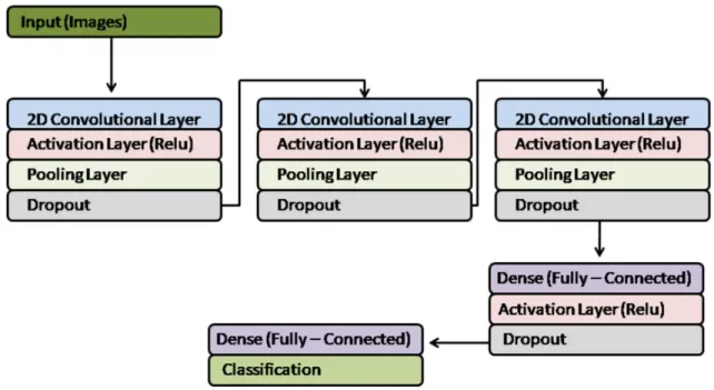
Deep convolutional neural networks contain an input layer, an output layer, and multiple hidden layers in between. The neural network is considered deep if there is more than one layer between the input and output layer, which are called hidden layers. Hidden layers are arraigned into groups called modules. Inside the modules, each layer performs a different function [27]. Modules generally consist of a convolutional layer, a pooling layer, and an activation layer. At the end of the network there is at least one fully connected layer. The

(29)

final layer in a network is a classification layer that labels the input image [34]. Figure 2-2 depicts a very simple deep convolutional neural network.

Figure 2-2: Basic Deep Convolutional Neural Network.

Convolutional layers extract features from their input [34]. Each convolutional layer has a receptive field which scans the input. The scan is convolved with learned weights to extract features and create a feature map [27]. An activation layer follows the convolutional layer and performs a manipulation to the feature map, producing an activation map. This enables extraction of non-linear features from the feature map. Pooling layers follow the activation layers and reduce the spatial resolution of the activation map. This results in spatial invariance to translations or distortions of the input [34]. Srivastava et. al. showed that dropout, random disconnection of a portion of the neurons in the network, makes a network less susceptible to overfitting, resulting in higher performance [19]. Dropout is common in convolutional neural networks following pooling layers.

At the end of a convolutional neural network there is at least one fully connected layer. In a fully connected layer each neuron is connected to every neuron in the previous layer. Fully connected layers also serve as feature extractors for higher level reasoning [34]. The final layer in a convolutional neural network is a classifier which outputs a label for the input data.

(30)

2.2.2 Convolutional Neural Network History

Convolutional neural networks trace their origin to the work of Hubble and Wiesel in 1959 and 1962 [17]. Hubble and Wiesel evaluated the response of cats’ brains to visual stimuli to determine the structure and operation of the visual cortex in their brains [21][22]. This work was the foundation of the biological relationship between artificial neural networks and neural networks in the brain of mammals [27]. The first notable use of a neural network based on Hubble and Wiesel’s research was by Fukushima in 1974 with a network named Neocognitron [17].

Neocognitron was a neural network consisting of a series of cells connected in a hierar-chical manner. The arrangement of the cells was similar to the structure of the visual cortex of cats discovered by Hubble and Wiesel [17]. Though not a convolutional neural network, as it lacked an end to end learning algorithm such as back propagation, this network was the predecessor to modern convolutional neural networks [27]. Neocognitron succeeded at identifying simple input patters, which is a rudimentary form of image classification [17].

The first reported use of convolutional neural networks was in 1989 by Waibel et. al. where a time-delayed convolutional neural network was used for speech recognition [27][49]. The first reported use of convolutional neural network for image processing was conducted in the early 1990’s in document reading systems. By the end of the 1990’s these systems were used for reading more than 10% of the checks written in the United States [43][27]. Between this time and 2012 there was limited reported use of convolutional neural networks. This was likely due largely to the substantial computation power required for convolutional neural networks and the fear that the networks would get stuck in poor local minima of the loss function during training, and therefore would not be optimized correctly [27].

In 2012, convolutional neural networks were accepted by main stream machine learning and computer vision learning communities after a convolutional neural network won the ImageNet competition [27]. LeCun et. al. suggest the key developments that enabled a convolutional neural network to win the competition were the use of graphics processing units (GPUs) for computation and rectified linear units (ReLu) as the activation function. The GPUs replaced central processing units (CPUs) for the computation and ReLus replaced sigmoid or hyperbolic tangent functions as the activation function [27]. These changes enabled faster computing with GPUs, conducting training 10-20 times faster than CPUs,

(31)

and ReLus conducting training six times faster than hyperbolic tangent activation functions [25][27].

There are emerging trends in the use of convolutional neural networks. Of particular note is the use of extremely deep networks to improve performance. Examples of extremely deep neural networks include GoogLeNet which consisted of 22 layers and won the 2014 ImageNet competition [38] and a network by MSRA which had 152 layers and won the 2015 ImageNet challenge [34]. Additional trends include developing networks that are easily deployed on mobile devices where storage and computation power are limited, as well as dealing with images that contain more than one label [34]. Improving model efficiency with respect to computation has historically been an area of active research and remains so today [34].

In addition to high end machine learning research, there is a trend to make machine learning more accessible through the use of specialized machine learning libraries. The use of dedicated machine learning tools streamlines the programming required for machine learning, allowing the programmer to focus on higher level network structure. The libraries optimized for machine learning include Google TensorFlow, Keras, Caffe, Theano, Scikit-Learn, and Tourch [36][4][1][32].

(32)

(33)

Chapter 3

Methods

This chapter outlines the methods used in this thesis. The experiment, signal processing, manual data evaluation, machine learning, other methods for diver detection, and physical modeling are each discussed in detail. The results of this analysis are presented in chapter 4.

3.1 Methods Overview

The first step in any supervised machine learning process is to generate a labeled data set. In this case data were collected with scuba divers at specified distances from a low-cost, passive hydrophone seaward of the WHOI dock. The acoustic data from the hydrophone was processed into spectrograms, a time-frequency image format, for human review. The data were then labeled and reformatted for machine learning.

Once an adequate labeled data set was available, a machine learning network was con-structed. Spectrograms for machine learning were created, and then split into three groups: training, testing, and validation. The data were feed into a machine learning network for training and tuning. The network produced a model capable of discriminating between data containing diver acoustic emissions and data which only contained background noise. After training, the network was tuned by adjusting parameters and evaluating the model’s performance. This process was repeated until an apparent optimum outcome was reached. Figure 3-1 is a flow chart depicting the overall process that is presented in the remainder of this chapter. The optimized model was tested against the validation data which had not been used in the training or tuning processes.

(34)

(35)

3.2 Experiment Setup and Data Collection

Acoustic data were collected at the WHOI pier when divers were present and when they were not. Divers followed a pre-determined testing protocol to ensure consistent data. Acoustic data were collected from a low-cost passive hydrophone near the WHOI dock and the data were recorded by a National Instruments Data acquisition unit topside.

3.2.1 Testing Site

Figure 3-2: Location of Hydrophone used in the Experiment.

The WHOI pier was chosen as the testing location both because it was convenient and because it is representative of a real-world port environment. Confounding factors include interfering surface vessels, noise from research ships moored at the pier, and noise from construction at the nearby Martha’s Vineyard ferry terminal. The hydrophone was placed in Vineyard Sound, the body of water between Martha’s Vineyard and Woods Hole. It was

(36)

approximately 6 m seaward of the southwest corner of the WHOI pier in 21 m of water. In this location it was less 25 m from the primary WHOI berth, which is used by Global and Regional class University-National Oceanographic Laboratory (UNOLS) vessels. The hydrophone was approximately 140 m from the Martha’s Vineyard Ferry Terminal and 600 m from the Ram’s Island pleasure craft anchorage. It was also directly adjacent to the entrance to the Eel Pond Anchorage. Figure 3-2 is a graphical depiction of the hydrophone’s location. The hydrophone was exposed to noise from vessels in Vineyard Sound, the Martha’s Vineyard ferries, construction noise adjacent to the ferry terminal, electrical noise from the WHOI pier, and ventilation and electrical noise from ships moored at the WHOI pier. The background noise at the hydrophone varied significantly from day to day and hour to hour. Vessels underway near the pier frequently masked the acoustic signature of scuba divers. For these reasons it would have been challenging to use traditional methods for diver detection that require a long integration time.

3.2.2 Equipment

The equipment used for data collection was a High Tech Incorporated (HTI) 96 min pre-amplified hydrophone. The pre-amplification improved the signal to noise ratio of the hy-drophone’s output and minimized the effects of the long cable, which was necessary for this experiment. It had depth rating of 3048 m (10,000 feet), frequency response from 2 Hz to 30 kHz, and a sensitivity of -240 dB. At a length of 6.35 cm and a radius of 1.9 cm the hydrophone was small in size. At a cost of $300 it is affordable for most applications even in quantity. The hydrophone was connected to a National Instruments DAQ series data acquisition unit located on the WHOI pier via a custom pi filter board.

The data were recorded in a Technical Data Management Streaming (TDMS) format which is the standard data format of National Instruments data accusation units. A file duration of one hour was chosen, enabling intuitive data processing and archival. With the selected recording settings, each one hour file was 1.688 MB in size. The recording settings are shown in table 3.1.

3.2.3 Testing Protocol

Data were collected by recording divers at known ranges from the hydrophone. A control data set was created by recording when divers were not in the water. A total of 20 dives

(37)

Table 3.1: Hydrophone Recording Settings.

were conducted near the hydrophone. The procedure outlined below was utilized by groups of two to three divers for data collection:

∙ Enter the water at the WHOI pier instrument well, located approximately 45 m from the hydrophone.

∙ Descend until approximately one meter above the bottom. ∙ Swim to the hydrophone, recording the time of arrival.

∙ Remain within 1.5 m (5 feet) of the hydrophone for 3 to 4 minutes, allowing time for the hydrophone to record the acoustic emissions from the divers.

∙ Swim to 3.05 m (10 feet) from the hydrophone and remain there for an additional 3 to 4 minutes. Record the time of arrival at this position.

∙ Repeat the preceding step in 3.05 m (10 foot) intervals, out to a distance of 15.24 m (50 feet), or until forced to conclude the dive due to diver bottom time limits.

On several occasions the procedure above was reversed with divers starting at 15.24 m (50 feet) from the hydrophone and moving closer to it every 3 to 4 minutes. A total of 7 divers, using at least 12 different sets of equipment, conducted the dives for this experiment. Over the course of the 20 dives 5,474 10-second spectrograms were generated; half containing divers and half containing only control data. A copy of the procedure and the data tables that the divers used is contained in appendix B. A list of all dives conducted and associated environmental conditions is in appendix A.

The maximum range of 15.24 m (50 feet) was chosen because it initially appeared to be the limit a human could detect a diver. In later dives, divers were occasionally detectable as soon as they entered the water, approximately 45 m from the hydrophone. A maximum

(38)

range of 15.24 m also allowed a diver to complete the entire testing protocol using air as their gas source without exceeding their no-decompression bottom time limit. Limiting range, and thus dive time, was also important during the winter months where dive duration is limited by environmental exposure using standard equipment. Safely extending range and bottom time in the winter would have required highly specialized equipment and training that were not available.

3.3 Signal Processing for Manual Evaluation of Data

Signal processing for this thesis was conducted in MATLAB. Machine learning was conducted as a second step using Python. The acoustic data were displayed in an image based, time-frequency format using the MATLAB spectrogram function. The spectrograms were saved as Portable Network Graphics (PNG) files for manual evaluation. Spectrograms were used because they displayed the frequency content of the signal with respect to time. This is the same format use by the Navy for target classification and is a proven method.

One minute spectrograms were chosen because this duration worked well for evaluation and classification by a human. Using one minute spectrograms divided the one hour long files into manageable chunks and was short enough to identify the characteristics of diver inhalation transients, the loudest acoustic source of open circuit divers [15]. The one minute duration of the spectrograms was only used for manual evaluation and was not related to integration time. Figure 3-3 shows a spectrogram containing emissions from three divers, 9.14 m (30 feet) from the hydrophone. The diver transients are visible for the first (bottom) 42 seconds and then are masked by the Martha’s Vineyard ferry getting underway.

Multiple permutations of spectrogram parameters were evaluated in an attempt to op-timize the detectibility of divers. The parameters presented in table 3.2 qualitatively opti-mized a human evaluator’s ability to detect the presence of divers. These parameters were kept constant throughout the thesis to maintain uniformity across the data. No filters were applied to the data, allowing evaluation of the entire 0-30 kHz spectrum.

3.4 Manual Evaluation of Diver Data

A data sheet outlining key parameters was recorded for each dive including the times that the divers were at each distance from the hydrophone as well as the time that they entered

(39)

Figure 3-3: Spectrogram from 1013 on 19 October 2018.

Table 3.2: Spectrogram Parameters.

and exited the water. Visual evaluation of data enabled reliable identification of the time when the divers arrived at less than 1.5 m from the hydrophone. Times on the data table were adjusted to match the time-base of the acoustic recording. The times provided by the divers and the times identified by manual evaluation often differed slightly, however they were never off by more than three minutes. This adjustment allowed the author to calibrate the data table to the acoustic recordings of the divers, enabling the author to determine the exact range from the divers to the hydrophone during the recording.

Spectrograms were evaluated for the duration of each dive to determine if a trained operator, the author, could detect the divers. If divers were identified the quality of the

(40)

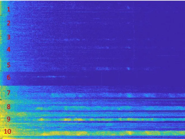
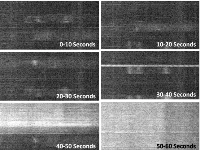
Figure 3-4: Combination of Multiple Spectrograms for Data Labeling. This Figure Was use to Assign a Quantitative Value to Diver Signal Strength During the Manual Data Review Process.

detection was quantified and documented. Appendix C is an example of the form used to record these data. The only human reviewer of the data was the author. It is likely that labeling errors were made; however, the risk of errors was minimized because the author knew when divers were near the hydrophone and when they were not and the author is highly trained and experienced in spectrogram interpretation. If errors were made they would have negatively impacted the network’s performance. Figure 3-4 is a combination of multiple spectrograms containing diver emissions with a numerical value correlating to the quality of the emission. This was used as the guide for quantifying the quality of the diver signature.

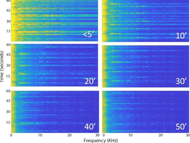
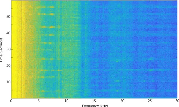
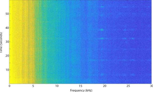
Analysis showed the quality of diver detection was dependent on the background noise during the dive and the range from the divers to the hydrophone. Figures 3-5 - 3-7 show the dependence of diver detection on both background noise, and distance. Figure 3-5 shows

(41)

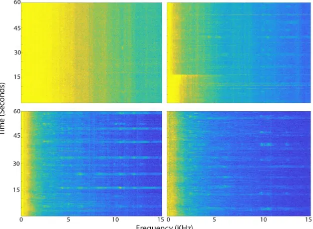
Figure 3-5: Diver Signature at 9.14 m (30 Feet) on Four Days. Top Left: 05 October 2018, Top Right: 19 October 201, Bottom Left: 26 October 2018, Bottom Right: 31 October 2018.

divers at the same distance, 9.14 m (30 feet), across four different days at different back-ground noise levels. Figure 3-6 depicts divers on the same dive, and at different distances, with low background noise. Figure 3-7 is the same as figure 3-6 except it shows a dive with higher background noise.

3.5 Data Labeling and Processing for Machine Learning

Data were prepared for machine learning by band pass filtering it and displaying it in 10 second spectrograms. Initially a single frequency band was chosen, however a second frequency band was later added for better detection in high background noise environments. The data were labeled and manually evaluated for later use in a machine learning network.

(42)

Figure 3-6: Diver Signature as a Function of Range with Low Background Noise. 31 October 2018.

(43)

Figure 3-7: Diver Signature as a Function of Range with Moderate Background Noise. 19 October 2018.

(44)

3.5.1 Initial Data Labeling and Processing for Machine Learning

An image processing approach for machine learning was chosen because it is a proven method for sonar classification. Additionally, to the knowledge of the author, an image processing, machine learning method for diver detection had not previously been evaluated. Spectro-grams were selected as the input for the machine learning network because they display the frequency content of the signal with respect to time. Spectrograms are the same tool used by the Navy for target classification with passive sonar.

Data from the first several dives indicated that the diver signature was most distinguish-able in the 10-13 kHz band. For this reason a band pass filter of 7.5-15 kHz with an order of 20 was chosen to filter the acoustic data. The data were displayed from 8-15 kHz. Though this range was generally the best, there were times when humans could detect divers outside of this range as shown in figure 3-8.

Spectrograms with a gray-scale color map and 10 second duration were utilized. The gray-scale color map was used because signal strength is directly proportional to intensity and therefore it was likely well suited for machine learning. The 10 second duration was cho-sen because it limited the number of diver transients in each spectrogram while maintaining a high likelihood that each would contain a diver emission. This minimized the complexity of individual spectrograms while ensuring they contained sufficient data for diver detection. One full spectrogram was required for diver detection, therefore reducing the spectrogram duration limited the required integration time. It is notable that Zhao et. al. also use a 10 second duration for their support vector machine diver detection system [51]. The fact that the sample length selected for this thesis matched the duration chosen by Zhao et. al. appears coincidental.

A MATLAB script was used to generate the spectrogram parameters discussed above. The script also cropped the images, to remove labels and titles. It automatically saved the spectrograms in a PNG format, placing applicable information in the file name. The information in the title included the date and time of the data, if there was a diver in the water at the time, the range of the diver, if there was a ship moored at the WHOI pier, the name of the ship, and a serial number representing the parameters used to construct the spectrogram. Appendix D contains a sample spectrogram title along with a key identifying the parameters in the title. Figure 3-9 shows the six, ten second spectrograms in the machine

(45)

Figure 3-8: Diver Signature 1001 18 December 2018 at a range of 3.04 m (10 Feet). The Bulk of the Diver Signature is Present Outside of the 8-15 kHz Band.

learning format from the 1013 minute of 19 October. Note this is the same data depicted in figure 3-3.

The spectrograms for machine learning were manually evaluated by the author to ensure each one contained a diver transient identifiable by a trained human. The spectrograms with divers in the water but not detectable by a human were segregated for later evalua-tion. In figure 3-9 the sixth spectrogram, from 50-60 seconds, was segregated because the diver transients were masked by the Martha’s Vineyard ferry. The other five spectrograms contained visible diver transients and were used in machine learning.

A control data set was generated by recording just before or after a dive when divers were not in the water. This data set was equal in size to the set containing divers. The data for the control set was within one hour of the dive to replicate the acoustic conditions of the dive as closely as possible. These data complemented the data containing diver transients, providing two data categories, one with divers, and one without.

(46)

Figure 3-9: Examples of Spectrograms in Machine Learning Format. Diver Range of 9.14 m (30 Feet) on 19 October 2018.

(47)

3.5.2 Additional Frequency Band for High Background Noise Environ-ments

Dives conducted on 19 December 2018 and 04 January 2019 contained minimal data where divers were detectable by a human in the frequency band of interest; however, divers were identifiable in higher frequencies. High background noise masked divers in the 8-15 kHz range and therefore a second frequency band of 18-25 kHz was instituted. The low frequency limit of 18 kHz was chosen because there was often a strong diver signature at approximately 19 kHz, and the high frequency limit of 25 kHz was selected to keep the spectrogram dimensions the same as the lower frequency band, making both bands compatible in the machine learning network. Previous data recorded at sufficiently high frequency was reprocessed at the higher frequency band, producing more data for machine learning.

Empirically it was noted that the lower frequency band was better for detection in lower ambient noise conditions, producing longer detection ranges due to less acoustic attenuation. The higher frequency band was better in elevated background noise, as 18-25 kHz was above the majority of the ambient noise near the WHOI dock. This is discussed further in section 5.1.2. Figure 3-10 is a spectrogram from 04 January 2019 where divers were not detectable in the original frequency band but were clearly visible in the higher frequency band.

3.6 Machine Learning

An overview of the machine learning process is shown in figure 3-11. The process began with splitting the data into three groups, training, testing, and validation. A machine learning model was trained using the training data and then tested with the testing data. The model was tuned by adjusting one or more hyperparameters and retraining the network. Hyperparameters are network parameters that are not learned during the training process and therefore must be sent manually prior to training. The training and testing cycle was repeated until an optimal model was produced. The validation data were then used to ensure that the model performed well on data that it had not previously been exposed to. When new data were produced it was first used to validate the model, then split into the initial three groups and the new, larger data set was used to produce a new model.

(48)

Figure 3-10: Spectrogram with Divers Only Detectable above 15 kHz. 04 January 2019.

Figure 3-11: Machine Learning Block Diagram. The Data Divide Splits the Data with 20% Becoming Testing Data. The Remaining 80% Becomes Training Data with a 90% Probability and Validation Data with a 10% Probability.

(49)

3.6.1 Machine Learning Data Split

Data for machine learning was split into three groups prior to training a model. The groups consisted of training data, testing data, and validation data. The training data were used to train the machine learning model. The testing group was used to evaluate the model’s performance during tuning. Following tuning the validation data were employed to verify the model performed well on data not used in the training or tuning process.

The original data set consisted of data from the eleven dives between 5 October 2018 and 30 November 2018. This data set contained 858 10 second spectrograms, half of which contained acoustic emissions from divers and half which did not. All of the data in this set was from the lower, 8-15 kHz, frequency band as the implementation of the higher frequency band occurred later. The intention was to use this data set to generate a preliminary model and to refine this model later when more data were available.

The data were spit such that the bulk was used for training the model. In general, it is recommended that the training set contain between 1,000-5,000 images of each class [36]. This was not possible with the original data set so the bulk of the data were placed in the training group to meet this recommendation as closely as possible. The data split was conducted randomly, using a Python script. Images had an 80% chance of becoming training data and 20% chance of becoming testing data. The validation data were taken from the training data, with a 10% chance that a training spectrogram would be shifted to the validation set and removed from the training set before any training took place. The end result was approximately 72% became training data, 20% testing data, and 8% validation data.

The training data were used to train new models and only used for this purpose. The testing data were used for model tuning which is described in detail in section 3.6.5. During tuning, hyperparameters in the network were adjusted and the model was evaluated against the testing data until optimal performance was achieved. The validation data were used after the model was tuned to ensure that it performed well on data that was not used in the training or tuning process.

As shown in figure 3-11, new data were initially tested using a previous model. This allowed the new data set to be used directly as validation data, evaluating how well the model properly classified new data. After validation the new data were then split with the

(50)

same probabilities as the original data set and added to the original data. The original data remained in its originally assigned category of training, testing, or validation. Specifically, once data were classified as training data, it remained training data for this entire process. The same was true for testing and validation data. The new, larger data set was then used to train a new model and the process repeated.

3.6.2 Machine Learning Metric Selection

Several choices for model tuning are available including to maximize the probability of detection, minimize the probability of false alarm, or a combination of thereof. The three primary metrics considered for optimization were precision, recall, and F1 score [39].

Precision is a measure of model’s ability to avoid false positives. It is the ratio between number of instances the model correctly identified as positive and the total number of instances the model identified as positive. Alternatively stated, for all instances classified as positive, precision is the fraction actually positive.

𝑃 𝑟𝑒𝑐𝑖𝑠𝑖𝑜𝑛 =

_{𝑇 𝑜𝑡𝑎𝑙 𝑃 𝑜𝑠𝑖𝑡𝑖𝑣𝑒𝑠}𝑇 𝑟𝑢𝑒 𝑃 𝑜𝑠𝑖𝑡𝑖𝑣𝑒𝑠

Recall measures the model’s ability to identify all positive instances. It is the ratio of true positives to the sum of true positives and false negatives. Alternatively stated; recall is the fraction of all positive instances classified correctly.

𝑅𝑒𝑐𝑎𝑙𝑙 =

_{𝑇 𝑟𝑢𝑒 𝑃 𝑜𝑠𝑖𝑡𝑖𝑣𝑒𝑠 + 𝐹 𝑎𝑙𝑠𝑒 𝑁 𝑒𝑔𝑎𝑡𝑖𝑣𝑒𝑠}𝑇 𝑟𝑢𝑒 𝑃 𝑜𝑠𝑖𝑡𝑖𝑣𝑒𝑠

The F1 score is a weighted harmonic mean between recall and precision where the best score is 1.0 and the worse score is 0.0. F1 is a balance between minimizing false positives and identifying all true positives. F1 score was the metric selected for optimization in the model tuning process.

𝐹 1 = 2

_{𝑃 𝑟𝑒𝑐𝑖𝑠𝑖𝑜𝑛 + 𝑅𝑒𝑐𝑎𝑙𝑙}𝑃 𝑟𝑒𝑐𝑖𝑠𝑖𝑜𝑛 * 𝑅𝑒𝑐𝑎𝑙𝑙

The choice to maximize F1 score was based on the lack of a specific penalty structure for this work. If there was an objective function, the choice of optimization may have been different. If the objective was detecting divers every time possible, independent of false alarm rate, recall would have been selected. Conversely, if there was a high penalty for false alarms compared to missed detection, precision would have been chosen. Taken to the

(51)

extreme either of these choices would have resulted in classifying every image as divers or every image as non divers. This would have resulted in no missed detections, or no false alarms respectively, but the model would have provided no value. With no clear objective function to optimize, maximizing F1 score appeared the most appropriate choice [41].

3.6.3 Machine Learning Software and Packages

Machine learning in this thesis was conducted in Python. Python was chosen because it is the programming language with the largest assortment of libraries designed specifically for machine learning [36]. The following python packages were used in the machine learning network presented later in the thesis. Figure 3-12 shows the inter-dependencies of the Python packages used in this thesis.

Figure 3-12: Python Package Inter-Dependencies.

Google TensorFlow

Google TensorFlow is a computational framework for building machine learning models [4]. It makes machine learning simpler and faster to implement [4]. TensorFlow is written with a python front end, simplifying programming, but conducts execution in C++ for better performance. The key benefit of TensorFlow is abstraction, allowing the programmer to focus on the higher-level machine learning implementation as opposed to the lower level

(52)

programming required for machine learning [50][5].

Keras

Keras is an application program interface (API) for high-level neural networks. Like Ten-sorFlow it is written in Python. A separate machine learning framework such as CNTK, Theano, or TensorFlow is required for Keras to function. TensorFlow was used as the back-end for Keras in this thesis. Keras was designed to be modular and allow for fast prototyping of neural networks. It supports both convolutional and recurrent neural networks, and can be run on either a central processing unit or a graphics processing unit [1][48].

Scikit-Learn

Scikit-learn is a machine learning library for classification, regression and clustering algo-rithms. In this thesis it was used for classification, determining the presence or absence of divers. Scikit-learn is written in Python. It requires several other packages including NumPy, SciPy, and Matplotlib [32].

Open Source Computer Vision Library (OpenCV)

OpenCV is a computer vision and machine learning software library that was used in this thesis for image processing tasks in machine learning. It was designed for real time computer vision. OpenCV has become de-facto standard for image processing in machine learning in recent years [36].

Imutils

Imutils is an image processing library that works with OpenCV. It was written by Dr. Adrian Rosebrock from PyImageSearch and provides functions for image processing [35]. In this thesis it was used for data augmentation, artificially increasing the size of the training data set, and to display results of model evaluation. Data augmentation is discussed in section 3.6.5.

Matplotlib

Matplotlib is a plotting library for python that produces two dimensional plots [2]. Mat-plotlib was used to plot the training process which for evaluation of over-fitting.

(53)

SciPy

Scipy is a set of numerical and scientific tools for Python. It is written in python but outputs to C++ binaries for more efficient execution. SciPy is used by several of the packages listed above [3].

Numpy

Numpy is a python library for multi-dimensional arrays. It enables Python to conduct efficient operations on arrays of data. Numpy is used by several of the packages listed above [3].

3.6.4 Network Overview

A deep convolutional neural network was used in this thesis. A straight-forward network was chosen for use on a standard laptop with minimal training time. Figure 3-13 is a graphical depiction of the network. The network was built using a Keras architecture. This convolutional neural network was similar in structure to a network used by Dr Adrian Rosebrock from PyImageSearch to evaluate root health of hydroponic plants [37]. That network was loosely based on AlexNet and OverFeat [41][25].

The network used in this thesis consisted of three modules of two dimensional convo-lutional layers followed by ReLu activation layers, pooling layers, and dropout layers. A module containing a fully connected layer, a ReLu activation layer, and dropout followed. The network was concluded with a second fully connected layer and a softmax classification layer. This architecture was chosen as it was straight-forward enough to be run on a com-mercial laptop while leveraging a modern deep convolutional neural network framework and using the most common activation function [27].

The convolutional layers extracted features from their inputs [34]. The initial convo-lutional layer extracted low level features from the image, but subsequent layers identified increasingly complex features [27]. The input of the first convolutional layer was a raw image. Subsequent convolutional layers used the activation map produces by the previous module as their input. Each convolutional layer had a receptive field which scanned the input. The scan was convolved with learned weights to extract features and create a feature map [27]. The feature map was smaller in dimension than the input as a result of the finite

(54)

Figure 3-13: Block Diagram of the Deep Convolutional Neural Network Used.

size of the receptive field used to scan the input. The convolutional neural network used in this thesis had a receptive field size of 7x7 for the first convolutional layer, 5x5 for the second, and 3x3 for the third.

A nonlinear activation ReLu was applied following each of the convolutional layers and the first fully connected layer. This layer increased the nonlinear properties of the previous layer and sets all negative values to zero. This allowed the network to extract non-linear features from the feature map [34]. The output of the activation layer was an activation map.

A pooling layer followed each of the activation layers. Pooling layers were effectively down-sampling layers, which took an input of neuron clusters of a given dimension from the activation map and output a single number. This resulted in spatial invariance to translations or distortions of the input [34]. In this thesis max pooling layers were used with an input size of 2x2. Max pooling used the highest of the input numbers as the output.

A dropout layer was included at the end of each module. The dropout layer set a random group of activations to zero. This is a form of regularization and helped minimize over-fitting [19]. Two sets of fully connected layers were included towards the end of the neural network. These layers connected every neuron in the previous layer to each neuron in the next layer.

(55)

Figure 3-14: Model Tuning Flow Chart.

The fully connected layers served as a feature extractor for higher level reasoning [34]. The last layer in the neural network was a softmax classification layer. The classification layer produced a probability distribution for the possible categories; diver or non-diver. This probability distribution was used to produce the final classification of each image.

3.6.5 Model Tuning

Model tuning followed network development. A model was trained with the training data set, then evaluated with the testing data set. One or more hyperparameters were then adjusted and the training and testing process repeated. This cyclic process was continued until a model with optimal performance was found. Two discrete models were developed during model tuning. The first, single frequency model, was produced from the 11 dives trough 30 November 2018, using data from the 8-15 kHz band only. The second, dual frequency model, was constructed from the 15 dives through 9 January 2019, using data from both the 8-15 kHz and 18-25 kHz frequency bands. Current best practice for all machine learning requires considerable tuning. This is one of the limitations of machine learning. Figure 3-14 is a graphical depiction of the model tuning work flow. Table 3.3 lists the key hyperparameters tuned for the network used in this thesis.