An asymptotic approach in the preliminary design of a launch vehicle control system

AN ASYMPTOTIC APPROACH IN THE PRELIMINARY DESIGN OF A LAUNCH VEHICLE CONTROL SYSTEM

by

PHILIPPE LE FUR

Ing6nieur de I'Ecole Polytechnique, Paris France (1986)

Submitted in partial fulfillment of the requirements for the degree of

MASTER OF SCIENCE in

AERONAUTICS AND ASTRONAUTICS at the

MASSACHUSETTS INSTITUTE OF TECHNOLOGY January 1989

@ Philippe Le Fur 1989

The author hereby grants to MIT permission to reproduce and to distribute copies of this thesis document in whole or in part.

Signature of Author

7/

Certified by

Department of Xronautics and Astronautics January 18, 1989

Professor Rudrapatna V. Ramnath Thesis Supervisor

Accepted by fi

Professor Harold Y. Wachman Chairman, Departmental Graduate Committee MASACHUSi1TS INSTITUTE of TECMHNtoeL Y WITHDR•AWN

j

MAR

10

1989

LIBRARIES

LBRARIES

I

AN ASYMPTOTIC APPROACH IN THE PRELIMINARY DESIGN OF A LAUNCH VEHICLE CONTROL SYSTEM

by

PHILIPPE LE FUR

Submitted to the Department of Aeronautics and Astronautics on January 20, 1989, in partial fulfillment of the requirements for the Master of Science in

Aeronautics and Astronautics

ABSTRACT

Gain scheduling is used in many engineering applications and particularly in aerospace engineering. The idea is to construct a flight control system for a linear slowly

time-varying system from a collection of local linear time-invariant designs. However, in the absence of a sound analysis, these designs can be unsatisfactory in regard to stability, robustness and performance.

This thesis shows how an asymptotic technique can be used to derive a feedback control system in a more rigorous way. The theory has been successfully applied to the preliminary design of a launch vehicle attitude control system. The Generalized Multiple

Scales (GMS) concept is invoked to generate a closed form solution to the time-varying system. This approximate solution is shown to be very accurate and is used to have more insight into the system. A "Minimum Drift Condition", derived by means of GMS theory in

[16], is stated and serves as a baseline for the control system. Implications of constant and variables gains are discussed in light of the GMS approach. Finally, recommendations are given for choosing the gains of the compensator to ensure performances as close as possible to the design specifications. These design guidelines would then be taken into account in a more advanced phase of the design.

A detailed presentation of the guidance and control problem, and extensive simulations, are also included in this work.

Thesis Supervisor: Dr. Rudrapatna V. Ramnath Title: Professor of Aeronautics and Astronautics

ACKNOWLEDGEMENTS

I would like to express my thanks to my research supervisor, Professor Rudrapatna V. Ramnath, for giving me the opportunity to work on the interesting problem of Multiple Times Scaling under his guidance. I also appreciated his valuable advice, interesting discussions and English instruction.

I am also very grateful to my parents and grandparents for their support, care and encouragement, which made this year at M.I.T. possible.

TABLE OF CONTENTS Abstract Acknowledgements Contents List of Illustrations Chapter 1 Introduction 1.1 Motivation 1.2 Objectives of Thesis 1.3 Organization of Thesis

Chapter 2 Mathematical Preliminaries 2.1 Background on Linear Systems

2.1.1 General Solution to a Linear System 2.1.2 Some Elements of Stability Theory 2.2 Approximation Theory

2.2.1 The Need for Approximation 2.2.2 Perturbation Methodology 2.3 Multiple Scales Methods

2.3.1 Introduction

2.3.2 Generalized Multiple Scales Method Chapter 3 Attitude Control of a Launch Vehicle

3.1 Problem Statenent 3.1.1 Introduction 3.1.2 Guidance System

3.1.3 Attitude Control System

3.1.4 Interaction of Control with Guidance and Loads 3.2 System Modeling

4.2 Analysis of the Homogeneous System 44

4.2.1 The GMS Solution 44

4.2.2 Investigation of Stability using GMS Approximation 54

4.3 Minimum Drift Condition Control Scheme 57

4.3.1 Minimum Drift Condition 57

4.3.2 Simplified GMS Solution 59

Chapter 5 Control System Trade -Offs

5.1 Introduction 65

5.2 Presentation of the Alternatives 65

5.2.1 Procedure #1 65

5.2.2 Procedure #2 68

5.3 Sensitivity Analysis 71

5.3.1 Sensitivity of Decoupled Roots 71

5.3.2 Sensitivity of Lateral Deviation 73

5.3.3 Implication for the Choice of Gains 74

5.4 Simulation Results 77

5.3.1 Introduction 77

5.3.2 Discussion of the Results 78

5.5 Limitations of the Foregoing Conclusions 80

Chapter 6 Conclusion and Recommendations

6.1 Conclusion 94

6.2 Recommendations for Future Work 94

References 96

Aopendix

A- DECOUPLING OF THE LAUNCH EQUATIONS 98

List of Illustrations

Frozen Approximation of the Solution to e

k

+

(1+t)x = 0

GMS Approximation of the Solution to E2*

+

(1+t)x = 0

Example of Turning Point

Elements of Guidance System

Schematic of a Pitch Plane Autopilot

Control Capability of the Attitude Control System

Reference Coordinates and Geometric Configuration

Attitude Control System Block Diagram

Vehicle and Flight Parameters

Dynamic Pressure vs Time

Open Loop System Response

Poles of Open Loop System

Examples of Feedback Gains

Real Part vs Time for the Three States, Casel

Imaginary Part vs Time for the Three States, Case 1

Real Root vs Time for the Three States, Casel

Numerical and GMS Solutions for the Three States, Case 1

Numerical and GMS Solutions for the Three States, Case 2

Real Part vs Time for the Three States, M.D.C. Case

Imaginary Part vs Time for the Three States, M.D.C. Case

Real Root vs Time for the Three States, M.D.C. Case

Numerical and GMS Solutions for the Three States, M.D.C. Case

Gain KA vs Time given by M.D.C.

Gain Ka vs Time given by M.D.C.

Feedback Gains vs Time given by Pole-Placement

Sensitivity of the Roots to Ke and KR

Sensitivity of rz3 to Ke and KR

39

48

72

Figure 5-7 Figure 5-8 Figure 5-9 Figure 5-10 Figure 5-11 Figure 5-12 Figure 5-13 Figure 5-14 Figure 5-15 Plots Plots Plots Plots Plots Plots Plots Plots Plots of 8, i and z - Test #1 of 0, a, 6 - Test #2 of 8, i and z -Test #2 of i and z -Test #3 of i and z -Test #4

of 0, a and 8 - Test #5 and Test #7

of Lateral Drift i -Test #5,6,7 and 8

of 0, a and 8 - Test #9 and Test #11 of Lateral Dritf i - Test #9,10,11 and 12

85 86 87 88 89 90 91 92 93

Chapter 1

INTRODUCTION OF THE THESIS

1.1 Motivation

The ultimate goal for control engineers is to design feedback control systems (also called controllers) that force the plant to conform to a desired behavior. Moreover, feedback can achieve the specifications even with disturbances and imprecise knowledge of the plant. One class of models for which both analysis and design are well understood is the class of linear time-invariant plants. For these systems, there are many techniques available in the literature ( Nyquist and Bode diagrams, root locus for Single-Input-Single-Output systems (SISO), Linear Quadratic Gaussian / Loop Transfer Recovery Methodology for Multiple-Inputs-Multiple-Outputs systems etc ...) thus allowing the design of a compensator to be systematic and relatively straightforward. Unfortunately, the systems encountered in the nature, and particularly in aerospace engineering, are rarely linear time-invariant thus requiring alternate methods for design of the controllers.

One popular method which has been extensively used is the "time slice" or "frozen" approach. The idea is to select several operating points which cover the range of the plant' s dynamics. Then, at each of them, the designer makes a linear time-invariant approximation to the plant and designs a linear compensator for each linearized plant. In between operating points, the parameters (gains) of the compensators are then interpolated, or scheduled (by time or any other exogeneous parameter such as dynamic pressure, velocity...), thus resulting in a global control system.

Even if such designs with gain scheduling work on many engineering applications, they come with no guarantee on nominal stability, stability robustness or command-following. Rather, any such properties are inferred from extensive computer simulations. In other words, a complete and systematic design methodology has yet to emerge.

1.2 Objective of the Thesis

A class of time varying systems of great interest, particularly in aerospace engineering, is the class of SISO linear slowly time-varying systems and the methodology developed in this report applies to this type of system only.

Most of the work has been carried on with a linear time varying system of order three representative of the motion of a launch vehicule about its nominal trajectory. Starting with this system, the objective is to find a compensator that is simple, relatively easy to implement, and comes with satisfactory stability properties and performances. Moreover, an important requirement is that the choice of the feedback gains must be such that the deviation from the nominal trajectory due to the wind be minimized.

The contribution of this thesis consists of: (1) analysis of a particular time-varying system by an approximation technique and (2) preliminary design of a gain scheduling flight control system.

First, the method of Generalized Multiple Scales (GMS) is invoked to analyze a linear time-varying feedback system. This method has been developed by Ramnath [12,13] for obtaining a uniform approximation of the solution to a slowly varying linear system. It provides for the independent variable (time for example) to be extended into a higher

dimension. This allows for a decomposition of the system behavior into a fast part and a slow part. The "slowly varying" stipulation requires that the system dynamics are much more rapid than the rate of change of the coefficients of the differential equation. This is true for the system under consideration in this study. The GMS approximation is shown to be very close to the numeric solution, which is representative of the exact solution. Of course, an exact analytical solution does not exist. The GMS approximation can then be used to derive more insight into the system behavior. In particular, it helps to analyze stability in a more rigorous way than the frozen approach does.

Secondly, this thesis makes recommendations for choosing the three feedback gains of a launch vehicle attitude control system. The GMS technique is once again used in order to find a condition on the gains that minimizes the deviations from the nominal trajectory due to perturbation and wind gust. This condition, first called the "Minimum Drift condition" in [7], has been shown to be valid throughout the time variation in [16] and not only at specific operating points as in [6,7]. It is also shown that the lateral drift can be further decreased by choosing the two other degrees of freedom in a proper way.

1.3 Organization of the Thesis

This thesis is organized into 6 chapters. In Chapter 2, some requisite background on linear time varying systems and approximation theory are presented.

Chapter 3 starts by presenting the problem of guidance and control of a launch vehicle. A simplified third order model, that allows the study of the interactions between control and trajectory deviation is then introduced and its main characteristics (time-varying, unstable ...) are discussed. Finally, the design requirements of the full-state feedback control system that is to be devised are specified.

In Chapter 4, the GMS technique is applied to obtain an approximate solution to the time varying system. This analytical expression (the GMS solution) serves as a starting point. It is first used to give conditions which guarantee the nominal stability of the system. A Minimum Drift condition is then stated [16] which is true continuously during all of the boost phase period.

Chapter 5 consists of recommendations, based on the results of Chapter 4, for the choice of the remaining gains. Two design alternatives are first presented. A sensitivity analysis is then performed on the relevant parts of the GMS solution that allows us to assess the superiority of one option over the other one. These conclusions are then validated by computer simulations of the overall system. A short qualitative discussion on the limitations of the present findings closes this part.

Finally, concluding remarks as well as recommendations for future work are given in Chapter 6.

Chapter 2

MATHEMATICAL PRELIMINARIES

2.1 Background on Linear Time Varying Systems

This chapter presents the general solution to a linear time varying system as well as some background material on stability theory. Emphasis is made on the fact that the tools and rules commonly used in linear time invariant theory can no longer be applied in

such a straightforward manner on this more general class of system. 2.1.1 General Solution to a Linear System

Consider the system described by the linear vector differential equation

X(t) = A(t).X(t) + B(t).u(t) (2-1)

Y(t) = C.X(t)

X(to) =Xo

The system is said autonomous or linear time-invariant (LTI) if A(t), B(t) and C(t) are constant (independent of time). Otherwise, it is called non-autonomous or linear time-varying (LTV).

Since the system (2-1) is linear, the solution can be found by first solving the

homogeneous equation and then applying the principle of superposition. For a non-zero initial condition Xo, the homogeneous (no input) solution to (2-1) is given by (see [3])

X(t) = QD(t, to). X _(2-2)

where 1(t,to) is called the state transition matrix associated with the matrix A(t) and has the following properties:

((t, to) = I

d _{(t, to) = A(t).A(t, to)}

dt (2-3)

The particular solution when u is not 0 is obtained by taking advantage of the linearity of the system.

If we choose X0 = 0 and integrate both terms of (2-1) from to to t, we obtain

X(t) = A(). X () do +

B

(t).u(r) dc

Sio

e(2-4)

Now, assuming u(t) is an impulse at t = s we have:

for t < s , (2-2) yields X(t) = 0

for t = s , (2-4) yields X(s) = B(s)u(s)

for t > s , (2-2) yields X(t) = F(t,s)x(s) = F(t,s)B(s)u(s)

Now we superpose all the responses due to the impulse u(s) from s = 0 up to s = t to get

X (t)

=

f t 0(t,r)B(t) dc

ito

The total solution for X0 * 0 and u # 0 is the sum of (2-2) and (2-5)

X(t) = D(t, to)Xo + ft D(t,t )B () dr

ito

and the output of the system is given by

t

Y(t) = C(t) D(t,to)Xo + fC (t)O(t, t)B () d(

(2-7)

The term H(t,t) = C(t)O(t,t)B(T) is called the impulse response matrix. For the particular case of LTI systems, C anb B are constant and it is readily seen that 0

(2-1) are also expressed in closed form. For LTI systems, we do have a closed form solution to (2-3):

(D(t, t) = eA(t-to)

On the other hand, it is important to note that for LTV systems, Equation ( 2-3) is very difficult to solve and very often unsolvable except for particularly simple systems. This formidable difficulty precludes the possibility of obtaining an analytical expression for the solution of an LTV system. As a result, other means, such as approximation techniques, must be used to come up with some sort of analytical expression that allows the engineer to have more insights in the system.

The Laplace transform theory proves to be very useful in the analysis of LTI systems. It is easy to manipulate and is such that, by inverting it, we can find the exact solution in the time-domain. For LTV systems, the Laplace transform cannot be used as simply to get the time-domain solution. To replace it, Zadeh [23] has defined the

system function as follows.

Consider the linear time-varying system represented by

u(t) [ LTV x(t)

System

and described by a differential equation between the output x and the input u

n m

I ak(t).ý xt x = bk(t). u(t)

k =

dz

k=O

dt

(2-8)

Introducing two functionals L and K with obvious significance, (2-8) can be rewritten as

L(4, t) x= K(d , t) u

dt dt

H(jw,t) = OW(t,t-t).e-jw d

where W(t,z) is the response at time t to a unit impulse at an earlier time z.

Note that if the parameters are constants (ak(t) = ak; bk(t) = bk), Zadeh's system function reduces to a plain Laplace transfer function from u to x (with s=jw).

We can show [23] that H(jw,t) satisfies the differential equation

n _{I akLw,t) •kH(jat) = Kjt)}

k=O ag)k a0 (2-9)

Similarly to the LTI case, it is shown that if a sinusoidal input is applied

u(t) = exp(jct)

the response of the system is

x(t) = H(j0,t).exp(jot)

so that for the frequency co, we can define the instantaneous gain and phase at time t as

IH(jA•t) and

However, Equation (2-9) cannot be solved in general except for very simple systems and it is the reason why Zadeh's system function has so far received very little attention in practical applications.

2.1.2 Some Elements of Stability Theory

under the following assumptions

(1) f is such that (2-10) has a unique solution over [to,oo) which depends continuously on the initial condition xo,to.

(2) f(x,t) = 0 for all t > 0. That is xe = 0 is an equilibrium state.

Notation * The notation s(t; xo,to) is used to denote the solution to (2-10).

11.11 is any norm on Rn and we define the norm of a function f(t) from R+ to

Rn by

Ilfll0

=

sup

IIf(t)ll

tto

Stability: The equilibrium state x, of the differential equation (2-10) is stable if for every real e there exists a positive real 8(E,to) such that

Ilx0ll1-

8

=• Ix(t x0,

toll0

.

-<

If 8 is independent of to, the stability is said uniform. If the property holds for all xo, the stability is said global.

AsvmDtotic Stability: The equilibrium state xe is said asymptotically stable if it is stable and if

lim

Ix(t; xo,

to

10

=

0

t ---oo

Attractivity : The system with initial condition xo at to is attractive if and only if, for all

E >0, there exists a number T (possibly dependent on the initial condition) such that

II x(t;

x,

to11

.5

E for all t-

o

T

i.e. attractivity is less strong than asymptotic stability in the sense that though it implies that all trajectories starting in a neighborhood of the origin eventually approach the origin, it does not require stability necessary.

Finally, consider a linear system of the form

dX= A(t).x

;

For an LTI system, we have the following criteria for stability:

* The system is asymptotically stable if and only if all the eigenvalues of A have strictly negative real part.

In general, this easy-to-use criterion cannot be applied to linear time varying systems and this is something we must keep in mind in this thesis. As a matter of fact, it is possible to find unstable systems for which the eigenvalues lie in the left half plane and vice-versa [4,21].

2.2 Approximation Theory

2.2.1 The need for approximation

Many of the problems faced today by the engineers involve difficulties such as nonlinear equations, variable coefficients and nonlinear boundary conditions at complex known or unknown boundaries which preclude their solutions exactly. For example, in the analysis of the flight of a launch vehicle, the variations in mass and density with altitude render the system highly time-varying. Similarly, in the transition from hover to cruise, a VTOL vehicle exhibits time-varying aerodynamic properties [14]. These two examples are parts of a large class of physical systems that can be accurately modelled by LTV systems for which we do not know the exact solution. Physical intuition,

experience as well as the use of powerful computers can generally give quite acceptable answers. However, in order to better understand the system, it is often needed to simplify it in such a way that conventional methods can be applied and yield an approximate solution.

As a matter of fact, approximations are universally resorted to, though often implicitly, and many of them are just ad hoc approaches. Now, a systematic as well as rigorous approach to approximation theory can be found in the subject of asymptotic analysis (studies in limiting cases).

A number of different techniques all related to asymptotic analysis have been developed by applied mathematicians and engineers. A formalization of asymptotic expansions and related concepts can be found in [10] and for more mathematical rigor the reader is referred to [5,8,11]. It is beyond the scope of this thesis to describe all of the available techniques but before introducing the one that is precisely used in this work, it may be interesting to discuss the main principle most of them are based on. 2.2.2 Perturbation methodology

Basically, in an asymptotic approximation, a small parameter E is identified and the problem is solved as E approaches 0. The solution of the unknown quantity is obtained in power of e as suggested by Poincar6 [11]. The approximate solution is represented by the first few terms of the asymptotic expansion, usually not more than two terms. For example, consider the second-order differential equation,

where (.) denotes differentiation with respect to t. with characteristic polynomial,

s2 + s + 1 =0 _(2-12)

To find the roots of this equation, we assume an expansion of the form

s(C)

=

s + E Sl + E2

Substituting (2-13) in (2-12) and collecting coefficients of like power of e, we obtain (sý + 1)+ e (2sosi + so)+... =0

where the ellipsis dots stand for all terms with power of en, n>l.

Since this equation is an identity in e, each coefficient of e vanishes resulting in a hierarchy of equations,

order 0 in e: order 1 in e:

S+ 1 =0

2sos + so =O

The solution of these equations is

so = +-

i

Sl= 2

Therefore, the first order solution to (2-12) is

S1, 2=i-

2

And finally, the solution to (2-11) can be approximated by

Since Equation (2-11) is solvable in closed form, we can check that our approximate solution is consistent with the true solution. The exact solutions of (2-12) are

Sl, 2=

2

An expansion in the small parameter e is now performed to give

2

E e

S1, 2= - fi.( 1 - +...)

Neglecting the terms in En for n > 1, we end up with

s1, 2= i-2

which is not surprisingly the same as (2-14).

This systematic procedure for solving approximate solutions of algebraic or/and differential equations of any order can readily be implemented on a computer and its usefulness is quite obvious if we consider that computers generally experience great difficulties in finding roots of equations where small and large numbers are mixed (stiff problem). However, this straightforward expansion (also called Poincar6 expansion) generally leads to a solution that is not uniformly valid and it breaks down in region

called " region of nonuniformity "[5,11,12].

To illustrate this phenomenon, consider a physical process represented by a slowly decaying exponential with the following governing differential equation

+Ex=O ; x(O)= 1 (2-15)

A straightforward expansion would yield

x(t)= 1 -et+e2t2 +...

whih.bvoulybrak..ow to t ofode

which obviously breaks down for t of order

-To render these expansions uniformly valid, investigators have developed a number of techniques. Among them we can cite the method of Strained Coordinates, the method of Matched and Composite Asymptotic Expansions, the Method of Averaging and the method of Multiple Scales. For a deeper understanding of the first three, the reader is referred to the cited references.

2.3 Multiple Scales Methods

2.3.1 Introduction

There are three variants of the method of multiple scales. In the first version (called "derivative expansion method"), Sturrock (1957,1963), Frieman (1963), Nayfeh (1965,1968), and Sandri (1965, 1967) showed that a uniformly valid expansion could be obtained by expanding the derivatives as well as the dependent variables in powers of the small parameter. The second version is due to Cole and Kevorkian (1963) and has been applied by Ashley [1] to conventional aircraft dynamics and by Kevorkian (1966) and Cole (1968) to several other examples. They obtained uniformly valid solutions by introducing two time scales linear in the original independent variable.

The theory has been generalized considerably by Ramnath [12,13] to include nonlinear scales which may also be complex quantities. Indeed, for a large class of problems such as those describing nonlinear and nonautonomous phenomena, linear scales are inadequate and the more general concept of non linear scales is necessary. By applying this powerful method, Ramnath developed uniformly valid approximations of the solutions of differential equations with slowly or rapidly varying coefficients [13]. This technique has been successfully applied by Ramnath and his students to various problems in the fields of flight and space dynamics [14,15,19]. More recently, Ramnath [28] has extended the Multiple Scales Method to include vector-matrix systems of differential equations.

2.3.2 Generalized Multiple Scales Technique (GMS)

The basic idea developed by Sandri and Ramnath is the concept of extension where the domain of the independent variable is extended into a space of higher dimension using suitable time scales or "clocks" depending on the small parameter E. The ordinary differential equation is converted into a set of partial differential equations which are functions of the independent scales. After equating like powers of e, the problem is solved order by order. By this means and a proper choice of the time scales, the non uniformities that arise in a direct perturbation method are eliminated and, furthermore, the fast and slow parts of the solution are systematically separated. Once the solution in terms of the independent variables is obtained, the time scales are expressed back in the original independent variable to give an approximate solution to the problem. The concept and solution development are illustrated by the following example.

Example

Consider the time varying differential equation,

E2 X + (l+t) x =0 _(2-17)

x(0)

=

xo

We know that for e = 1, the exact solution to Equation (2-17) is the Bessel function of order one third J1/3(t). It is a higher transcendental function that cannot be written in terms of simple functions. The search for an approximation is now undertaken.

The independent variable t is first extended into two time scales to and 'l with

o= t ;

i=

k(u)du

(2-18)

The derivative with respect to t are then transformed into

d - k

- •-- 0 + e-

2 2 1 - ( -1 + t1

2k

at

l

1 2a2

These variables transform (2-17) into a partial differential equation

k2 2x k2I It

ax

+ E. (k

c

+ 2k a)

azoazl

+E

+ (1+Co)

x

Coefficients of like powers of e are collected and equated to 0, resulting in a hierarchy of equations,

k2 ax + o0x = 0

1 (2-19)

The form of the solution is now assumed to be

x = A(to).exp(tl)

slow part fast part

Substituting (2-21) into (2-19) determines the clock function k to be solution of, k2 + (1+r0) = 0

or k =

+

(2-21)

(2-22)

Substituting (2-21) and (2-22) into (2-20) yields a differential equation for A 1 (1+ro)j A(ro) + 2 (1+to)2 dA =0

2 dzo

which gives, after integration

d >

a

-- > -a +

X(t,E)

=

(1+t)

-1/4.

Cl sin(

_(1+t)3/2)

₊

_c2

_cos(

₂

_(1+t)3/2

₍

3 3 (2-23)

The GMS method has the interest of providing a formula for an approximate solution which explicitly separates the slow and fast parts. More precisely, the fast part of the GMS solution, which is in the example,

X(t,E) = Cl sin(2 _(l+t)3/2_{) + c}

2 cos( 2 (1 +t)3/2)

3 3

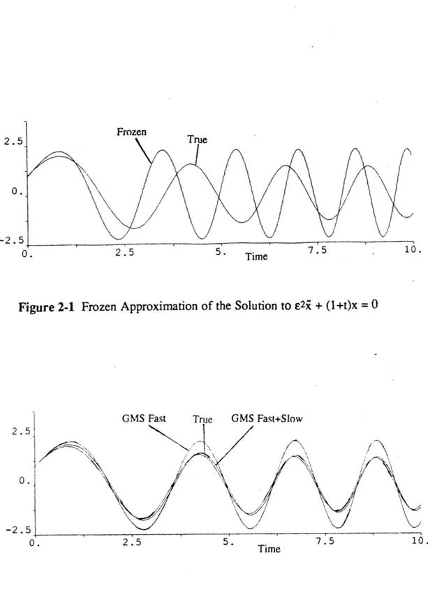
shows the "frequency" variation of the solution whereas its combination with the slow part also shows the "amplitude" variation of the solution. The combination of the two parts form a composite solution which is in general very close to the real solution as it can be seen in Fig. 2-lb. Also, in Figure 2-la we have plotted the "frozen" solution which is obtained by solving (2-24) as a second order differential equation with constant coefficients. This leads to the solution,

X(t,e) = c, sin((1+t)) + c2 cos(((l+t)!)

Clearly, this approximation is very bad. Neither does it represent the phase nor the

amplitude variation. It is therefore misleading and of total uselessness.

This was just a simple example to show the possible decomposition of an event into various rates and its particularity accurate GMS approximation.

Pictorially,

. SOLUTION

2.5

0.

-2.5

I I1lil

Figure 2-1 Frozen Approximation of the Solution to e2i + (l+t)x = 0

2.5 0. 0. 0. 2.5 5. _Time 7.5

I

I

I

Generalization

The GMS solution for a general nth-order differential equation with slowly varying parameters has been derived by Ramnath in [13].

Such an equation can be written in the form,

an(t) x(n)(t) + an-l(t) x(n-1)(t) + ... + ao(t) x(t) = 0 (2-24)

where (.) denotes differentiation with respect to t and with the assumption that the quantities

ai(t) are slowly varying functions of time.

Mathematically, it is tantamount to saying that the coefficients ai(t) vary on a new

slow time variable t = et where e is a small positive parameter being a measure of the ratio of

the time constants of the dynamic motion and the coefficient variations. Making the change of

variable t = et , Equation (2-24) becomes

Enan(t) x(n)(t) + en-lan-l(t) x(n-1)() + ... + ao(t) x(t) = 0 (2-25)

where (.) now denotes differentiation with respect to t.

In order to develop an asymptotic solution when E tends to 0, Ramnath extends the variables t into a set of two independent variables,

t - To = t; ₁ '= k[i](t) dt

0 ~(2-26)

Following the same mathematical manipulations as in the example treated previously , we can

derive the Oth order GMS solution as,

n X

I(o0') = c i e[i]

i= 1 (2-27)

or again back in the original space,

n

S(t) = C i exp( k[i](u) du)

i=l _(2-28)

where - the ci are dependent upon the initial conditions

Sam(r)

k

_{= 0}

As solution given by (2-27) is the fast scale solution, it primarily describes variations in frequency and phase of the solution. More accuracy on the amplitude variation can be obtained by including the slower behavior as well, i.e. by including the first-order

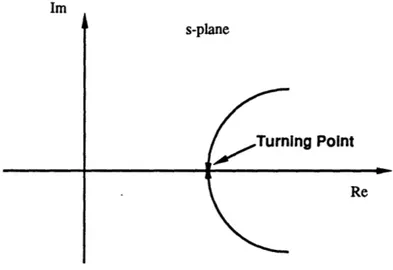
solution[13]. By doing so, the coefficients ci would become functions of the slow time scale; ci(to). If the system is such that the characteristic roots approach each other but do not coalesce, inaccuracy may arise in the approximation of the phase of the true

solution. When the roots do coalesce, the phenomenon is called a turning point. At such a point, the dominant and subdominant terms of the asymptotic approximations switch roles. This disturbance to the ordering of the term does not allow the asymptotic series to accurately represent the solution on both sides of the turning point. Further analysis involving hyperbolic functions is required to allow a multiple scales approximation to match the true solution around a turning point. For further detail, the reader may consult the discussion by [12,9].

The ~ - Transfer Function

An ordered hierarchy of transfer functions for slowly varying linear systems was developed by Ramnath [16] and is illustrated as follows. Consider the LSTV system with scalar representation

n m

ai(t) dt i=

i=

o

di i=

o

with ai(t) slowly varying _(2-29)

The Oth-order equation is given by

n I

ai(To)

By definition, the Laplace transform of the function x(to,tl) with respect to tl is

L {(x(To,tl)) = X(s) = e-s

T'

By Laplace transforming both sides of (2-30), we obtain

Y

i=

m

si X(s) =

I

i=0

Now, the Laplace clock space variable is defined [16] as

=

sk

Finally, we obtain a " k-transfer function " that relates the fast parts of u and x as (2-31)

(t)-Y

X_= =o _{=G(ý, To)}

u

ai(To) i

i =O (2-32)

At this point, it should be noted that the poles of the function G(j,to) play an important role in the undriven case (no input). Indeed, if those poles are denoted by k('ro), (k =

1,...,n) the homogeneous solution can be approximated by

n

(t) =

•

k 1 r J'0) where the constants rk depends on the initial conditions.

Ramnath [16] applied this theory to the problem of controlling the space shuttle during boost and used it to derive the condition for minimum lateral drift.

Chapter 3

LONGITUDINAL CONTROL OF A LAUNCH VEHICLE

3.1 Problem Statement

3.1.1 Introduction

The performance quality of a space launch vehicle during the launch phase of flight is generally studied in two distincts, though related phases. The first deals with the trajectory of the vehicle with reference to some specified inertial frame and is called

the Guidance problem. It is mainly concerned with such issues as payload capacity,

dispersions from nominal, and orbit capability. In this context, the vehicle is usually assumed to be a point mass and the oscillations about nominal trajectory have a "low frequency" behavior. However, the action of the control system in orienting the vehicle in the required position is not instantaneous. In general, the control commands induce oscillations about the center of mass and these must be damped out if the mission is to be successful. This is the Flight Control System problem, the subject matter of the vehicle "short period" dynamics. The following formulation of the problem and the related discussion is based on the work by Greensite [6].

3.1.2 Guidance System

In the design process of an automatic control system for launch vehicle, one first deals with the trajectory equations and with the relationship between between guidance philosophy, control response and trajectory profile. The main result of this study is the development of a reference trajectory that describes ideally the motion the vehicle from launch to either earth impact or orbit injection. The general formulation includes all effects that are known to be significant for purpose of guidance and control: among these are nonspherical rotating earth, variable mass of vehicle, eccentric center of gravity and jet damping. Conversely, such higher order dynamic effects as fuel sloshing, bending,

gyro and actuator dynamics are neglected. The development of trajectory equations has its foundation in the classical theories of celestial mechanics and the equations of rigid body motion. More advanced guidance laws can also be derived with application of

variational calculus and optimization theory. While certain approximations for specific purposes are immediately evident, it must be recognized that the manipulation of the equations to simplified form is often an art rather than a science, based heavily on experience and engineering judgement. As a consequence, virtually all aerospace contractors and government agencies have developed trajectory equations that are usually tailored for specific needs or missions.

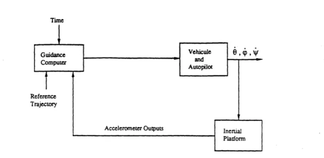
The essential elements of a guidance system are shown in Figure 3-1. The guidance system must:

a. Measure the position and velocity of the vehicle (Navigation).

b. Evaluate this information in the sense of determining if the vehicle position vector is indeed on agreement with the stored reference trajectory (Computation).

c. Generate steering signals that incorporate corrections for deviations (Control). Typically, the signals generated by the guidance system are in the form of roll rate *ic(t), and attitude rate in pitch 0c(t) and yaw 4c(t) . These three signals are the inputs to the vehicle Autopilot. However, for the sake of simplicity, we will assume the desired trajectory to lie in a vertical plane so that only the attitude rate command in pitch, also called pitch program, will be considered in the analysis.

As a matter of fact, for purposes of guidance, the attitude or attitude rate is not the primary quantity of interest. In the guidance problem, the 0 input to the autopilot is applied in order to control the velocity vector displacement of the vehicle. The use of attitude rate command is effective in steering to a desired acceleration direction because a change in attitude results in approximately the same change in direction of the vehicle acceleration vector. This follows from the fact that the predominant force acting on the vehicle is thrust which is always constrained to lie a few degrees of the vehicle longitudinal axis. This is equivalent to saying that the angle-of-attack is very small or that the vehicle does not fly but is rather only boosted along its trajectory. However, in the presence of winds, aerodynamic forces caused by changes in the angle of attack will result in the vehicle drifting off the desired trajectory. To reduce these acceleration errors, various approach have been used by conventional systems. This will be discussed in more depth in Section 3.1.4.

3.1.3 Attitude Control System

The guidance system provides the control system inputs necessary to fly a prescribed trajectory. These inputs are generally in the form of attitude commands

whose purpose is to orient the vehicle properly. In conventional launch vehicle autopilots, the function of the Steering Loop is to control the attitude rate and the function of the Flight Control System is to control the attitude in response to an attitude command supplied by the steering loop. With these two principles in mind, the

schematic of Fig. 3-2 corresponds closely enough to the actual hardware implementation of a conventional single-channel Autopilot.

The attitude control problem is concerned with the short period dynamics of the vehicle where the fundamental aim is to achieve adequate stability and reasonably rapid (well-damped) response to input commands, with moderate insensitivity to external disturbances (winds and other sensor noise).The distinguishing features of the attitude control problem of a launch vehicle are:

a. The use of swivelled engines for attitude control. b. Aerodynamic instability of the airframe.

c. The extreme flexibility of the vehicle. d. The influence of propellant sloshing.

e. The varying mass and inertial properties of the vehicle.

The first requirement of the attitude control system is that there exists sufficient control capability to counteract anticipated aerodynamic loads. Referring to Figure 3-3 and following Greensite [6], this requirement can be formulated quantitatively by

Tcmnaxlc > Lala 0mnax (3-1)

where

Tc = control thrust

La = aerodynamic load per unit angle of attack

Ic = distance from mass center of vehicle (cg) to engine swivel point la = distance from mass center of vehicle to center of pressure (cp)

8 = thrust deflection angle

a = angle of attack

In short, the thrust control moment must be larger than the maximum anticipated aerodynamic force. Based on a maximum available thrust deflection angle 8max, a

maximum permissible angle-of-attack onax can thus be determined which in turn limits the weather conditions that the vehicle can safely flies through.

Major design problems arise because a launch vehicle is aerodynamically unstable and hugely flexible. The problem that requires most care is probably that of vehicle flexibility, which manifest itself in the sensing of undesirable local elastic deflections by the gyroscopes. When the bending mode and control frequencies are of the same order of magnitude, potential stability problems exist. The use of passive filters is needed but other problems may arise by the fact that these filters compromise the gain and phase margins of the control loop and that the bending-mode frequency vary in flight.

Further complications are due to the sloshing of liquid propellants and the inertia effects of swivelling engines.

Last but not less important, the flight parameters and inertial properties vary during the flight. In conventional designs, this makes use of the so-called "time slice" approach, in which all the parameters are "frozen" over a short period of time, about a specific operating point. With this artifact, classical linear control tools are used to derive a sequence of adequate flight control systems each of them being characterized by a set of gains. In between operating points, the flight control system switches from one set of gains to another using time or dynamic pressure as gain-scheduling

parameter. Of course, though these kinds of flight control systems do work in practise, they come with no guaranteed performances and extensive time-varying simulations on computers are necessary to make some refinements and finally validate them. As it has been pointed out in the introduction, one purpose of this thesis is precisely to introduce the multiple scales method as a means to derive a time-varying flight control system in a more rigorous way.

The first stage in designing an attitude control system is to make a rigid body analysis to determine performance characteristics (drift, loading, response time) and to come along with order of magnitude for the gains of the control system. The second phase is concerned with the flexible body analysis to determine filters and gyro locations as well as to refine the values of the gains.

3.1.4 Interaction of Control with Guidance and Loads

The usual method of studying the short period motion of a launch vehicle is to analyse perturbations from a reference conditions via linear method and to design an autopilot configuration that meets the specifications. Though this problem can be

analysed to a large extent independently of the guidance considerations, the two cannot been completely divorced. As a matter of fact, the characteristics of the autopilot will have a significant influence on trajectory dispersions and on the vehicle loading, especially during the atmospheric phase where the vehicle is subject to high dynamic pressure and high velocity wind disturbances. Indeed, if the vehicle attempts to follow the pre-specified trajectory in the presence of large wind disturbance, the angle of attack may be significantly increased, resulting in a large aerodynamic normal force as well as some lateral drift in the wind direction. This large aerodynamic force, in combination with the thrust component normal to the vehicle to balance the torque produced by the aerodynamic force, can cause large bending moments which the vehicle may not be able to withstand. These normal forces to the vehicle can be reduced almost completely through "load relief' schemes [7] that cause the vehicle to rotate into the wind so as to reduce the angle of attack and the corresponding loads. But these schemes lead to large deviations from the nominal trajectory [6].

In conclusion, in addition to achieve adequate short-period stability, the vehicle flight control system will be required to meet two conflicting requirements:

,(i) to minimize trajectory deviations since excessive guidance corrections result in payload penalty.

(ii) to minimize the angle-of-attack excursions in order to reduce the resulting bending moment or in other words, ensure structural integrity of the vehicle.

Depending on which requirements the emphasis is made on, the control system structure will be quite different.

This present work is mainly concerned with the general features of the attitude control problem, especially as they relate to trajectory deviations. The problem of

minimizing the angle of attack excursion could not be accommodated within the time and scope constraints of this thesis but would of course require attention in a secondary design stage.

Time

Figure 3-2 Schematic of a Pitch Plane Autopilot

Lcia

Figure 3-3 Control Capability of the Attitude Control System

3.2

System Modeling

3.2.1 Vehicle Model

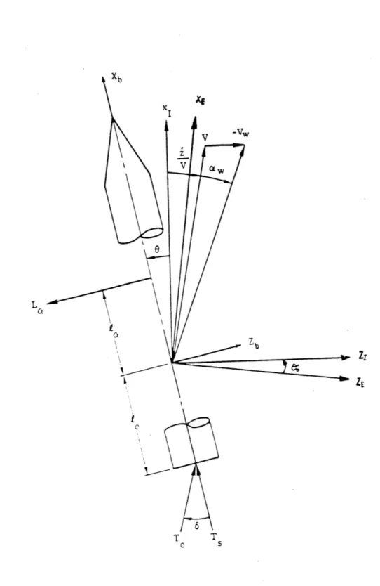
There are many possible frames of reference to represent the forces and moments that influence the motion of the vehicle in its pitch plane. The three sets of axes used in this study are shown in Figure 3-4.

a. The earth-fixed coordinate frame (XE, ZE) which coincides with the trajectory plane with the XE-axis and the ZE-axis coincident with the local horizontal and vertical lines of the earth at the launch pad.

b. The non-rotating vehicle reference system (Xb, Zb) where the Xb-axis lies along the longitudinal axis of the vehicle, positive in the nominal direction of positive thrust acceleration. The Zb-axis completes for a standard right-handed system.

c. The trajectory inertial system (XI, ZI) that is tangent to the nominal trajectory of the vehicle. It is obtained from the earth-fixed coordinate frame by a rotation of 00

(nominal attitude) about the ZE x XE-axis.

The motion of the vehicle in the pitch plane can be studied with reference to Figure 3-4. Neglecting the effects of bending and sloshing and the lags due to actuator

and instrumentation, the linearized equations of motions of the vehicle have been derived in detail in [6] and take the form:

2= [T + gcos(00)]0 LaTc 6 0 = •a + P'8

ax =0

+ +

a•w

(3-2)

where

D = drag

I = moment of inertia of vehicle about pitch axis

m = mass of vehicle

XE v V L a: ZE ZE i C T T T T c s

0 = attitude angle error relative to trajectory inertial frame.

Oaw = gust angle of attack = - Vw/V

and other symbols are as defined previously.

During the flight, all the vehicle parameters and flight conditions change as time evolves. The variations of these coefficients are primarily due to changes in dynamic pressure (Figure 3-6), velocity, aerodynamic force and moment parameters. Typical time histories are listed in Table 3-1. These data have been measured in an actual flight and refer

to a space shuttle launch vehicle. At this point, it should be noted that these coefficients can be considered as slowly varying so that the use of the "frozen" approach and later on of the

"Multiple Scales" approach can find justification.

3.2.2 Feedback Control

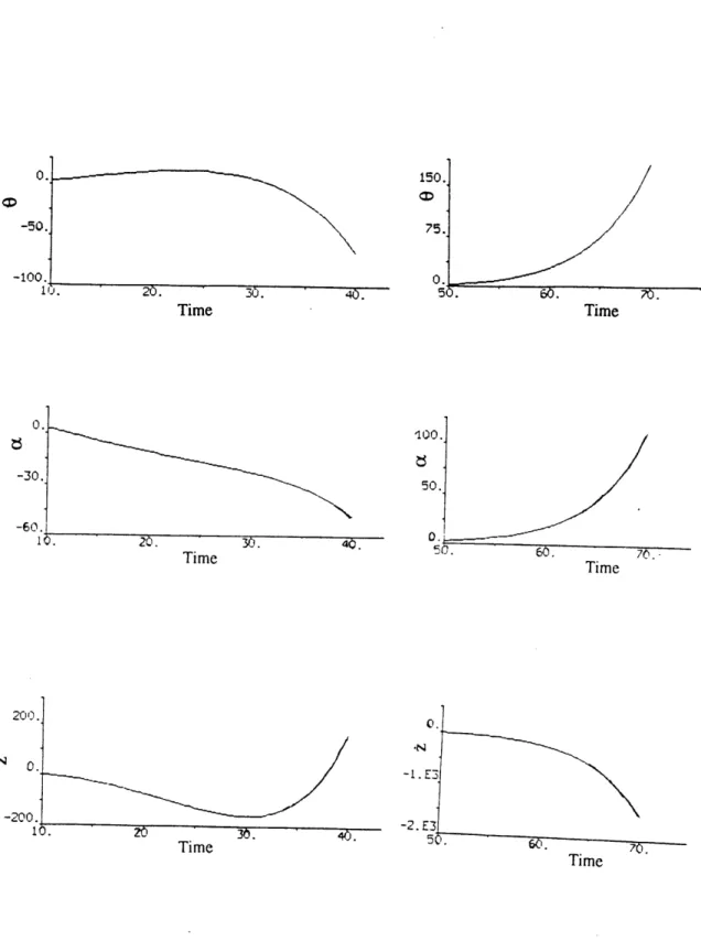
In the absence of any control input, the vehicle is unstable as it can be seen in Figure 3-7. This shows the attitude, angle of attack and lateral drift response of the vehicle to initial conditions on 00 (3 deg) and 00 (1 deg/sec) at t = 10 and 50 seconds. Also shown in Figure 3-8 are the time histories of the three eigenvalues of the open loop system when t varies from

5 sec. to 140 sec. The two complex conjugate roots essentially represent the short-period mode of the vehicle and are associated with the rotary motion of the vehicle about its center of gravity. It is interesting to note that they coalesce at 52 and 110 seconds. The third root is always real and describes essentially the response of the flight path (i/V) to the wind. These three roots lie well in the right half plane during all the flight duration and not surprisingly cause the vehicle to be unstable.

The primary role of the attitude autopilot will be to stabilize the vehicle. This will be done by moving the two complex roots in the left half plane in such a way that the resulting short period mode has a sufficiently short period and an acceptable damping. The second task of the autopilot will be to move the real root as close as possible to zero. To achieve these two goals, we will use a control law that feeds back three measurable outputs of the system; the attitude angle 0, the pitch rate 6 and the angle-of-attack a. Following [6], the

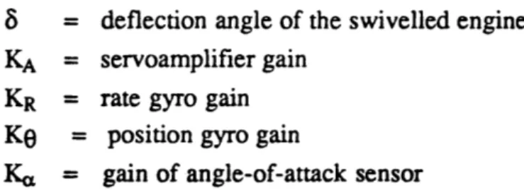
8 = deflection angle of the swivelled engine

KA = servoamplifier gain

KR = rate gyro gain

KG = position gyro gain

Ka = gain of angle-of-attack sensor

Although the pitch rate is relatively easy to obtain by means of a simple conventional rate gyro, the two other quantities are generally available from rather complicated instruments called "estimators". It is beyond the scope of this thesis to discuss on the principles of these devices. In reality, the outputs of these estimators result from intense computations and are corrupted by all sorts of undesirable noise that limit both their availability and their accuracy. However, in this work, and for purpose of simplicity, the measurements of 0, 6 and ca will be considered as perfect (free of noise) and instantaneously available (no lag due to instrumentation or signal processing).

In summary, the model of the closed-loop system which is formed by combining the vehicle and the attitude control system models is depicted in block-diagram in Figure 3-5. The output variables 8, 6 and a of the vehicle model provide the input data for the controller. The output of the controller is a commanded nozzle deflection 8 which serves as the input to the vehicle model.

Reference Input Disturbances

The following set of parameters of a generic launch vehicle is based on the work of Ramnath [16] on the space shuttle.

= 5.17 - 0.0417t ft = (77.08 + 0.0417t) ft = (323 - 1.55t).106 slug-ft2 - 1.712.105 - 815t slugs = Sref = 3420 ft2 - 32.2 ft/sec/sec - 3.21 lbs/radian - 0.2 lbs/radian

= Effective control thrust for attitude control

= 5.92.105 lbs = t2exp(-1.72 + 9.75.10-3t - 2.76.10"t 2) = t(5.46 +0.18t) fps = (893 - 1.43t).104 _lbs = Drag = 684q lbs = CLSq = 10980q lb/radian

=

Table 3-1 Vehicle and Flight Parameters

la(t)

m(t)

CLta

Cd

TC

q(t)

0. -50. -100. Time 0. -30. -60. 120. _{30. 4} Time 150. 5v. Time '100. 50. 0. 50. 60. 70 Time 200. 2N 0. -_{2 0 0}.j Time

Figure 3-7 Open Loop System Response

Time

-. C -. 2 -. 25 -. 3 0 30 60 90 120 150 TIME 3 30 50 90 120 o50 16 14 06 .0 .02 0 -.02 D 30 60 90 120 150 TIME .14 .D_ .02 0: -05 - CE -.09 - 12 12 .09 05 6-.0 -. 09 -. 12 J. 7 --.UD 1~

3.3 Design specifications

In summary, the primary role of an attitude autopilot is to stabilize the vehicle and to control the attitude angle. It is also of prime importance to minimize the deviations from the nominal trajectory and to limit the induced angle-of-attack in response to winds. These requirements can be presented in the form of design specifications numbered from 1 to 7.

Specification 1: The compensated system must exhibit a good stability behavior in

response to a perturbation that deviates the states from 0. The settling time (time after

which the error in 0 is less than, say, 0.5 deg) must be acceptable.

Spiecification 2: The gains of the compensator must be such that the deviations from

the nominal trajectory are minimized.

Specification 3: For a typical non-zero initial states and a typical wind profile, the thrust angle deflection (control) must not exceed a maximum allowable value 8max.

Specification 4: The gains of the feedback systems must not be too large to avoid amplification of the sensor noise and excitation of the unmodelled dynamics.

Specification 51 The angle-of-attack excursion must be minimized to avoid loss of control and excitation of the bending modes.

Specification 6: The Flight Control System must have good command following in the

range of low frequency for compatibility with guidance law.

Specification 7: In order to be reliable and not expensive, the control system must be easy to implement.

As it has been pointed out in Section 3.1.4, a trade-off must be made between

Spec 2 and Spec 5. The final decision must be made by considering the specific mission

(what is worst tolerable deviation from the nominal trajectory at the end of the flight?) and the structural configuration of the airframe (what is the maximum lateral force that it can withstand?). Solving such a trade-off is of course out of the scope of this thesis. Rather, the emphasis has been put on the problem of minimizing the deviations from the trajectory (Spec 2).

Chapter 4

APPLICATION OF MULTIPLE SCALES

4.1 Introduction

In Chapter 2, we have outlined the Generalized Multiple scales method and its potential applications to control theory. In Chapter 3, we have discussed the problem of designing an autopilot for a launch vehicle. In the first section of this part, we apply the GMS method to first obtain a closed form solution to the time-varying system and then consider some conditions for stability. In Section 4.3, we state the "Minimum Drift

Condition" that has been derived in [16] by means of Multiple Scales. This is a condition that the gains must satisfy in order to minimize the deviations from the nominal trajectory.

4.2 Analysis of the Homogeneous System

4.2.1 The GMS Solution

In this section, we study the stability behaviour of the undriven system with neither reference input nor external disturbance.

By introducing the state vector

x=[t, 0,

(4-1)

the equations of motion (3-2) can be written in state space form

the closed loop system can be written as

X(t) = Ac(t).X(t) ; X(to)= Xo _(4-4)

The closed-loop characteristic roots of the system are determined by solving the characteristic polynomial of Ac, namely

det(sI - Ac) = 0

which is a third order equation with respect to s of the form (t0 = t)

s3 + B₂(T,)S 2 _{+ BI(r1)s + Bo(To) = 0}

(4-5a)

with

B2(To) = IcKAKR + T' (KAKa + _{mv TC} (4-b)

(4-5b)

B1(To) = .cKA(KO + Ka) - pa + KAKRTc _{mv y} + PC)

(4-5c)

KAKT

La

La

Tt-D

gcos(

0)

Bo(to) m AO + Pc) - v ).(cKAKa a) (4-d)

Though linear, the system of three first order differential equations (4-4) cannot be solved exactly because it is non-autonomous. However, as it has been pointed out earlier in Section 3.2, and with the additional assumption that the gains do vary slowly

also, these coefficients can be considered as overall slowly varying. This fact motivates the use of the GMS technique to derive an approximate solution.

The first step to generate the closed form solution is to decouple the system (4-4). For this third order system, the algebraic manipulations have been very

cumbersome and are not given in this work due to space limitation. The final result is a set of three third order homogeneous differential equations of the form

iRi + CilXi + Ci2.i + Ci3.xi = 0 (4-6)

Note that the time dependent coefficients Cij (i, j = 1..3) contain several derivatives of the coefficients aij of the matrix Ac. They are given in appendix A.

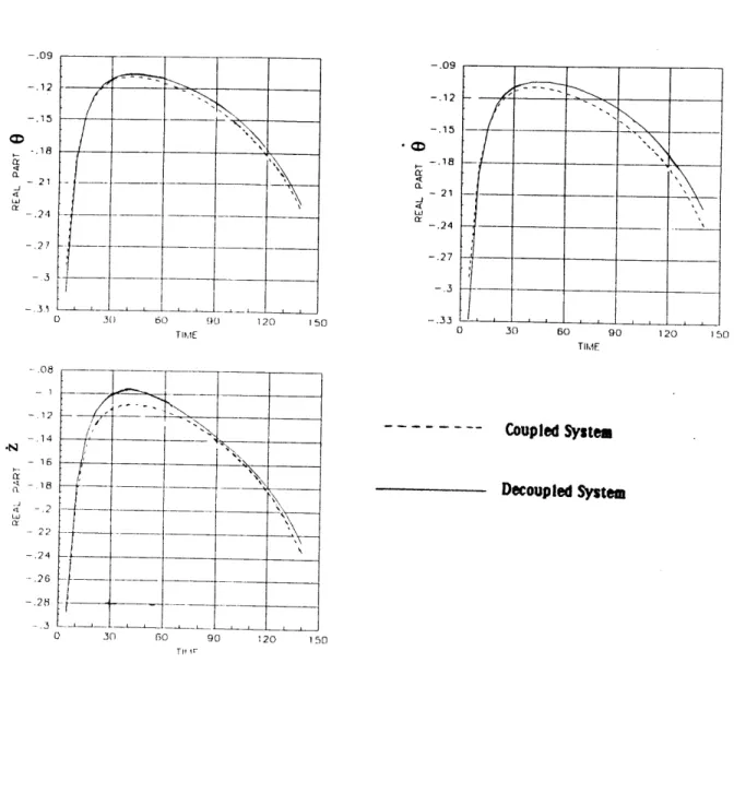
The characteristic polynomial corresponding to (4-6) has three roots. For all reasonable feedback, it can be shown that two of the roots are complex conjugate and the other one is real. For the first set of gains tabulated in Table 4.1, the real part and the imaginary part of the complex roots and the real root of the polynomials

corresponding to each of the three differential equations (4-6) have been plotted as functions of time in Figures 4-1 through 4-3. Also plotted are the eigenvalues of the original matrix Ac for reference.

Table 4.1 Examples of feedback gains

The characteristic root trajectories show that the decoupled characteristic roots for each state are similar but not identical to the eigenvalues of the coupled system. This difference is of course due to the rate of change of the coefficients in the decoupled equations and is particularly noticeble on the real part of the complex roots and on the real root.

The next step in deriving the GMS solution is to generate equations in

parametric form for the real and imaginary parts of the roots. In general, it is impossible

to derive analytical forms of the roots of a polynomial of order greater or equal to 5. For

polynomials of order 3 and 4, the Tartaglia-Cardan method can theorically be used to get the exact analytical expression of the roots. However, this method requires a lot of algebra and some tests of positiveness at some stage that have prohibited its use in this work (not easy to implement). An alternative would be to list the root locations

Case KA Ke KR Ka

1 1 3 1 0

- .09 -. 12 -. 15 -. 18 - 21 2 -. 24 -. 27 -. 3 -.33 o 3T) 60 90 120 150 o 30 60 90 120 150 TIME Coupled System Decoupled System 0 30 50 90 120 15D

Figure 4-1 Real Part vs Time for the Three States, Casel -.09 -. 12 -. 15 -.18 -21 -24 -.2,7 -. 12 .14 - 16 -16 -. 2 -22 - .24 .26 .28 -3 -.3. -.0

a at C-30 50 90 1 -c L Ju ,U 90 120 15() Coupled System Decoupled System 0 30 5• Y 1 0O 1.4 1.3 1.2 11 .9 .8 7 [1 1.2 t.1 1 · r

.4 .35 .3 * 3 .25 0 .2 g .15 .1 .05 O 0 0 30 60 90 1 0 1 f0 TIME 0 30 60 90 1: Coupled System Decoupled System 30 60 90 1 0 150

Figure 4-3 Real Root vs Time for the Three States, Casel

However, one class of feedback systems for which this assumption proves to be quite accurate is that corresponding to the Minimum Drift Condition which is introduced in Section 4.3.1. This third method for evaluating the roots will therefore be presented in Section 4.3.2.

For each of the states we have now three root trajectories. For example for 0 we have:

k

0

l(t)

=

k

r(t)

+ ikei(t)

k

(t) = ker(t)

-

ikei(t)

KO

(t)

f

ker(t)dt + i. kei(t)dt

Ke

(t) =

ker(t)dt - i.

f

kei(t)dt

The Oth-order GMS approximate solution to Equation (4-6) then becomes 6(t) = z₁.exp(Ker+ iKei) + z2.exp(KO -iKei) + z3.exp(K03)

where the zi's are complex constants dependent on the initial conditions. The solution can be rewritten as

0(t) = exp(Ker(t)).( i.(zl -z2).sin (Kei(t)) + (zi + z2).cos (Kei(t)) ) + z3.exp(K03(t))

Since 0(t) is real, the imaginary part must cancel and therefore z1 and z2 are complex conjugate. Finally, the expression for 0(t) can be written as

t

i tt t

0(t)

=

rl.exp( ker(t)dt). sin( kei(t)dt) + r2.exp( kr(t)dt). cos( kei(t)dt )

+ r3.exp( k3(t)dt) (4-7)

where rl, r2 and r3 are real valued coefficients dependent on the initial conditions.

The same procedure is used to generate multiple time scales solution to z and 0. Further, an approximate solution to the deviation z(t) can be obtained by just

integrating i(t)

(4-8) and an approximate solution for the angle of attack cz(t) is obtained as follows

2(t)

a(t)= =(t) +

v (t)

_(4-9)

The determination of the coefficients ri's is not a particular difficult task but requires

some care. This is not done here for sake of conciseness but the interested reader may

refer to Appendix B for more detail.

On the following pages (Figures 4-4 and 4-5) are the superimposed plots for the

GMS solution and the true numerical solution to the three states of the system for the

two cases of Table 4.1. The numerical solution has been generating from a computer

program (Simnon) using a fourth order Runge-Kutta algorithm with automatic

2.5 -2.5 0. ) 0. -0. -5. i A 40. Time 80. 120 A B 40. Time 80. 120 · ~ __ _ 1

3. -0. -3. . 4 0 . TIME (sec) 8 0 . 12 0

1.5

Figure 4-5 Numerical and GMS Solutions for the Three States, Case 2

I -- . "-~-I 1--- --- " -` --- ---