Column Generation Approaches to the Military Airlift
Scheduling Problem
by
Mark J Williams
B.S. Operations Research, US Air Force Academy (2012)
Submitted to the Sloan School of Management
in partial fulfillment of the requirements for the degree of
Master of Science in Operations Research
at the
MASSACHUSETTS INSTITUTE OF TECHNOLOGY
June 2014
This material is a declared work of the U.S. Government and is not subject to
copyright protection in the United States.
Author . . . .
Sloan School of Management
June 2014
Approved by . . . .
Allison Chang
Technical Staff, MIT Lincoln Laboratory
Technical Supervisor
Approved by . . . .
Mariya Ishutkina
Technical Staff, MIT Lincoln Laboratory
Technical Supervisor
Certified by . . . .
Cynthia Barnhart
Chancellor
Ford Professor of Engineering
Massachusetts Institute of Technology
Thesis Supervisor
Accepted by . . . .
Patrick Jaillet
Dugald C. Jackson Professor
Department of Electrical Engineering and Computer Science
Co-director, Operations Research Center
Column Generation Approaches to the Military Airlift Scheduling
Problem
by
Mark J Williams
Submitted to the Sloan School of Management on June 2014, in partial fulfillment of the
requirements for the degree of Master of Science in Operations Research
Abstract
In this thesis, we develop methods to address airlift scheduling, and in particular the problem of scheduling military aircraft capacity to meet ad hoc demand. Network optimization methods typically applied to scheduling problems do not sufficiently capture all necessary characteristics of this problem. Thus, we develop a new method that uses integer linear programming (IP) with column generation to make the problem more tractable while incorporating the relevant characteristics. In our method, we decompose the problem into two steps: generating feasible aircraft routes, and solving the optimization model. By ensuring that routes are feasible with respect to travel time, ground time, crew rest, and requirement restrictions when we build them, we do not need to encode these characteristics within the IP optimization model, thus reducing the number of constraints. Further, we reduce the number of decision variables by generating only the fraction of feasible aircraft routes needed to find near-optimal solutions.
We propose two methods for generating routes to include in the IP model: explicit column generation and selective column generation. In explicit column generation, all aircraft routes that we could potentially consider including in the model are generated first. Starting with a subset of these routes, we iteratively use reduced cost information obtained by solving a relaxed version of the IP model to choose more routes to add from the original set of routes. In selective column generation, we first generate a small set of feasible aircraft routes. Starting with this set of routes, we iteratively generate more routes by solving a relaxed version of the IP model and then combine routes in the solution together and add those that are feasible to the route set. In both methods, we iterate until there are either no other routes to include or the solution stops improving. Last, we solve the IP model with the final set of routes to obtain an integer solution.
We test the two approaches by varying the number of locations in the network, the number of locations that are wings, and the number of requirements. We show that selective column generation produces a solution with an objective value similar to that of explicit column generation in a fraction of the time. In our experiments, we solve problems with up to 100 requirements using selective column generation. In addition, we test the impact of integrating lines of business while scheduling airlift and show a significant improvement over the current process.
Technical Supervisor: Allison Chang
Title: Technical Staff, MIT Lincoln Laboratory Technical Supervisor: Mariya Ishutkina
Title: Technical Staff, MIT Lincoln Laboratory Thesis Supervisor: Cynthia Barnhart
Title: Chancellor
Ford Professor of Engineering
Acknowledgments
This thesis would not have been possible without the support of many people. First, and foremost, I must thank my MIT advisor, Cynthia Barnhart, for her guidance and encouragement along the way. I am fortunate to have had the opportunity to learn from such a caring and knowledgeable person and I am grateful for all of her time.
I owe a tremendous amount of credit to my MIT Lincoln Laboratory advisors, Mariya Ishutkina and Allison Chang. I truly appreciate all of their thoughtful feedback and support throughout my research. I have learned a great deal about problem solving from each of them. I hope to see you during my next assignment the next few years.
Thank you to all of the students and faculty that have helped me along the way. I appreciate all of the help in coursework, seminars, and research to get to this point. I am especially grateful to Jon Paynter for his feedback on my thesis.
I thank the U.S. Air Force and MIT Lincoln Laboratory for allowing me the opportunity to pursue this degree. I look forward to serving and hope to make a positive impact.
Last, and certainly not least, I am forever indebted to my family, especially my parents, for their love and support in all my endeavors. I especially thank Kristen for her love and patience the past several years.
The views expressed in this article are those of the author and do not reflect the official policy or position of the United States Air Force, Department of Defense, or the U.S. Government.
Contents
1 Introduction 10
1.1 Contributions . . . 11
1.2 Thesis Structure . . . 11
2 Background and Literature Review 13 2.1 Background . . . 13
2.2 Current Planning Process . . . 16
2.2.1 Strategic Planning . . . 16
2.2.2 Mission Planning . . . 17
2.2.3 Sources of Uncertainty . . . 18
2.3 Proposed Planning Process . . . 18
2.3.1 Problem Definition and Assumptions . . . 20
2.3.1.1 Network . . . 21
2.3.1.2 Requirements . . . 21
2.3.1.3 Aircraft and Aircrew . . . 22
2.4 Literature Review . . . 22
2.4.1 The Network Design Problem . . . 23
2.4.2 The Pickup and Delivery Problem . . . 23
2.4.3 Airlines . . . 24 2.4.4 Related Efforts . . . 25 3 Arc-based Formulation 27 3.1 Related Work . . . 27 3.2 Time-expanded Network . . . 28 3.3 Arc-based Model . . . 29 3.3.1 Sets . . . 30 3.3.2 Parameters . . . 31 3.3.3 Decision Variables . . . 32
3.3.4 Formulation . . . 32
3.4 Summary . . . 34
4 Route-based Formulation 35 4.1 Related Work . . . 35
4.1.1 The Pickup and Delivery Problem . . . 35
4.1.2 Column Generation . . . 36
4.2 Aircraft Route Generation . . . 37
4.2.1 Path Generation . . . 39 4.2.1.1 Examples . . . 41 4.2.1.2 Algorithm Tactics . . . 43 4.2.2 Route Generation . . . 45 4.3 Route-based Model . . . 50 4.3.1 Sets . . . 51 4.3.2 Parameters . . . 51 4.3.3 Decision Variables . . . 52 4.3.4 Formulation . . . 52 4.4 Column Generation . . . 53
4.4.1 Explicit Column Generation . . . 54
4.4.1.1 Dual Formulation . . . 54
4.4.1.2 Reduced Cost . . . 55
4.4.1.3 Reduced Cost Approximations . . . 56
4.4.1.4 Solution Strategy . . . 57
4.4.2 Selective Column Generation . . . 58
4.4.2.1 Generating Initial Routes . . . 58
4.4.2.2 Solving the Subproblem . . . 58
4.4.2.3 Advantages . . . 59 4.5 Flexible Model . . . 60 4.5.1 Sets . . . 60 4.5.2 Parameters . . . 60 4.5.3 Decision Variables . . . 61 4.5.4 Formulation . . . 62 5 Computational Experiments 64 5.1 Data and Assumptions . . . 64
5.1.1 Network . . . 64
5.1.3 Aircraft and Aircrew . . . 67
5.1.4 Costs . . . 67
5.2 Route Generation . . . 68
5.3 Model Scaling . . . 71
5.4 Integrated versus Segregated Scheduling . . . 73
6 Conclusion 75 6.1 Summary of Results and Contributions . . . 75
6.2 Future Work . . . 76
A Logic for P OT EN T IAL 78
B Logic for SEQU EN CE 79
C Logic for F EASIBLE 81
D Logic for DOM IN AN T 92
List of Figures
2-1 US Transportation Command organization . . . 14 2-2 Organization of the 618th Air and Space Operations Center (TACC) . . . 15 2-3 Scheduling timeline for a typical requirement . . . 17 2-4 Hypothetical probability density function and cumulative density function
describ-ing the likelihood a requirement will change dependdescrib-ing on the number of days until execution. . . 19 2-5 Hypothetical histogram of the number of requirements known based on the number
of days until execution . . . 20 3-1 An example of a dynamic network where the labels on the arc represent travel times 28 3-2 Time-expanded version of the network in Figure 3-1 . . . 29 3-3 Time-expanded network with a sink node and artificial arcs for one commodity and
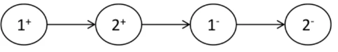
one wing at port D . . . 32 4-1 This path covers requirements 1 and 2 and is not empty until the final stop . . . 38 4-2 This route consists of two paths with an empty flight segment in between and it begins
and ends at the same wing . . . 38 4-3 Sequence of a possible path with the travel times between ports . . . 42 4-4 A simplified example of the impact limiting paths by the number of requirements has
in the case of delays . . . 45 4-5 Limiting the number of possible route combinations based on proximity. In this
example, there are only five possible locations reachable in one move from the location in the center. . . 46 4-6 Once a partial route length exceeds the threshold, we add the original route if its
origin and destination are closer together than the origin and destination of the new route. Otherwise, we continue to add paths to the new route. . . 49 4-7 We will try to complete a partial route if the origin and destination are in close
4-8 Column generation approach . . . 54 5-1 Ports considered for use in our experimental network . . . 65 5-2 Average time to build paths based on the number of requirements in the path . . . . 68 5-3 Average time required to generate paths and routes based on how we limit paths . . 70 C-1 Sequence of a possible path with travel times . . . 89
List of Tables
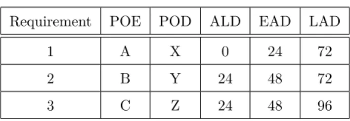
4.1 Requirement data . . . 41
4.2 Earliest arrival and departure times . . . 42
4.3 Inflated latest arrival and departure times . . . 43
4.4 Latest arrival and departure times . . . 43
5.1 Per unit cargo type specifications . . . 66
5.2 Partial aircraft cargo mix . . . 67
5.3 Limiting paths has minimal affect on solution quality and reduces the computational time necessary to generate routes dramatically . . . 69
5.4 Comparison of explicit and selective column generation for small test problems . . . 72
5.5 Summary of results for selective column generation in large problems . . . 73
5.6 Comparison of scheduling requirements aggregated with scheduling requirements by LOB . . . 74
Chapter 1
Introduction
The United States Transportation Command (USTRANSCOM) is responsible for a global supply chain comprising multiple modes of transportation and numerous stakeholders. The airlift network is a vital portion of their supply chain. Airlift requests, called requirements, vary from Presidential movements to natural disaster relief and the lead time to schedule such requests range from hours to months. Each requirement specifies a pick up location, delivery location, time windows restricting when the cargo can be picked up and delivered at each location, as well as size and type of cargo to be transported.
Scheduling these requirements is challenging for a couple of reasons. First, the problem is highly dynamic in terms of both demand and resources. Second, the volume of requirements makes it difficult to schedule. Third, identifying requirements with potential to be scheduled together is challenging for a human because the opportunities depend on the time and locations of the pick up and delivery location as well as the size of the cargo to be transported [15].
Requirements are currently scheduled in a manual process by flight planners. Flight planners are divided by lines of business (LOBs), each of which schedule requirements of one type because of the large number of requests. As a result, flight planners have no knowledge of other LOBs even though they are utilizing the same set of limited aircraft, crew, and airport resources. In addition, flight planners wait to schedule requirements until two weeks prior to execution because the requirement data tends to stabilize at this point.
In this thesis, we propose a scheduling framework based on optimization in order to produce a single airlift schedule and utilize the limited resources efficiently. We develop an integer linear programming formulation that is able to aggregate requirements both within and between LOBs to schedule all requirements at once. Furthermore, we implement two column generation approaches to reduce the size and complexity in order to address the large number of airlift requirements.
1.1
Contributions
We make the following contributions in this thesis:
• We develop an algorithm to generate aircraft routes that are feasible in terms of travel time, ground time, and requirement time restrictions in order to reduce the size and complexity of the optimization model. We demonstrate that the use of dominance criteria to eliminate routes that serve the same requirements and utilize the same aircraft type does not have a significant impact on solution quality.
• We develop the deterministic Route-based model, an integer linear programming (IP) opti-mization model that is able to aggregate all types of requests to create a baseline schedule. In addition, we present an alternative, the Flexible model, by modifying the Route-based model to allow for flexibility in the departure and arrival days for aircraft.
• We implement two column generation approaches to further reduce the size of the optimization model: explicit column generation and selective column generation. We show that neither of the two approaches consistently performs better in terms of solution cost, but selective column generation produces a solution in a fraction of the time compared to explicit column generation. As a result, we are able to solve instances with up to 100 requirements using selective column generation.
• While we implement techniques to produce a schedule resilient to change, we provide the framework to develop a robust Route-based model to incorporate the level of uncertainty in the problem.
1.2
Thesis Structure
The organization of this thesis is as follows.
In Chapter 2, we motivate the problem by describing the current scheduling process and propose a scheduling framework suitable for the characteristics of the problem while allowing the opportunity for optimization. We introduce relevant terminology while describing the available data and the necessary constraints that characterize the military airlift scheduling problem. In addition, we review the pertinent literature and relate it to our problem.
We introduce traditional network formulations and relate relevant work in the literature to our problem in Chapter 3. We develop an optimization model based on this using a time-expanded network. We conclude by discussing the tradeoffs with using this type formulation.
In Chapter 4, we reformulate our model to tackle the challenges from using a traditional network formulation. We begin by relating relevant approaches taken in the literature to our problem. Next,
we describe our algorithm to generate feasible aircraft routes and the corresponding optimization model. In addition, we explain the two column generation approaches we employ and formulate an alternative optimization model.
We design computational experiments to test the performance of our approaches in Chapter 5. We report on how well our model scales and discuss the tradeoffs in using different parameters to reduce the solve time. In addition, we evaluate the benefit of aggregating request types in creating aircraft routes.
Finally, we conclude by summarizing our keys results and suggest future work to build upon our contributions.
Chapter 2
Background and Literature Review
The United States Transportation Command (USTRANSCOM) is responsible for a global supply chain comprising multiple modes of transportation and numerous stakeholders. The airlift network is a vital portion of their supply chain. Airlift requests vary from Presidential movements to natural disaster relief and the lead time to schedule such requests range from hours to months. Scheduling is challenging due to the number of requests, the size of the transportation network, and the many practical constraints unique to the problem. Creating an efficient schedule is necessary to provide timely airlift to support these critical missions.
The remainder of the chapter is organized as follows. We provide general background information on USTRANSCOM in Section 2.1. In Section 2.2, we detail their current planning process and the challenges presented by the military airlift scheduling problem. We propose a planning process to overcome those challenges in Section 2.3. We conclude with a brief review of the pertinent research in the literature describing solution approaches to similar problems in Section 2.4.
2.1
Background
USTRANSCOM is a Department of Defense (DOD) unified command. A unified command is a military organization with a “broad continuing mission under a single commander and composed of significant assigned components from two or more Military Departments” [18]. The DOD orga-nizes unified commands by their geographic responsibility or by the function they provide to the geographic Combatant Commands (COCOMs). USTRANSCOM is a functional command with a mission to “provide full-spectrum global mobility solutions and related enabling capabilities for supported customers’ requirements in peace and war” [34].
USTRANSCOM relies on multiple modes of transportation to provide those mobility solutions. Figure 2-1 depicts how USTRANSCOM is organized. It consists of two subordinate commands-the Joint Enabling Capabilities Command (JECC) and the Joint Transportation Reserve Unit
(JTRU)-Figure 2-1: US Transportation Command organization
USTRANSCOM
US Transportation Command
AMC
Air Mobility Command
SDDC
Military Surface Deployment and Distribution Command
MSC
Military Sealift Command
JECC
Joint Enabling Capabilities Command
JTRU
Joint Transportation Reserve Unit
as well as three componenet commands-Surface Deployment and Distribution Command (SDDC), Military Sealift Command (MSC), and Air Mobility Command (AMC). This thesis focuses on the airlift portion of operations, which is largely the purview of the 618th Air and Space Operations Center, primarily known as the Tanker Airlift Control Center (TACC), and Air Force wings.
USTRANSCOM partners with commercial carriers to provide additional capacity. This is done using the Civil Reserve Airlift Fleet (CRAF) for air transportation. Commercial airlines participat-ing in CRAF commit a portion of their passenger and/or cargo fleet to augment military airlift in emergencies [25]. Once notified by TACC, the carriers have 24 to 48 hours to have their aircraft ready. In exchange, the government makes peacetime business available to those airlines.
USTRANSCOM is responsible for the distribution and deployment of DOD personnel and cargo. Because we focus on airlift operations, the relevant USTRANSCOM responsibilities include [34]:
• Partner with the geographic COCOMs in the planning and execution of military support to stability operations, humanitarian assistance, and disaster relief, as directed;
• DOD’s single manager for transportation responsible for providing common-user (i.e., other than service-unique or theatre-assigned assets) and commercial air, land, and sea transporta-tion; terminal management; and aerial refueling to support the global deployment, employ-ment, sustainemploy-ment, and redeployment of US forces; and
• DOD Distribution Process Owner (DPO) responsible for coordinating and overseeing the DOD distribution system to provide interoperability, synchronization, and alignment of DOD-wide, end-to-end distribution and developing and implementing distribution process improvements that enhance the defense logistics and Global Supply Chain Management System.
Figure 2-2: Organization of the 618th Air and Space Operations Center (TACC)
TACC
618th Air and Space
Operations Center XOZ Director of Operations XOB Mobility Management XOC Command and Control XOG Global Channel Operations XOW Global Mobility Weather Operations XOO Current Operations XON Mission Support XOP Global Readiness
In fiscal year 2012 (FY12), AMC executed 31,181 airlift missions delivering 1,882,495 passengers and 659,176 short tons (stons) of cargo to carry out those responsibilities [34]. Distribution involves mov-ing sustainment supplies and accounts for approximately sixty percent of all AMC movements [26]. Although the distribution process can be difficult to forecast, it is much more similar to commercial supply chain networks than deployment. AMC classifies distribution movements as Channel mis-sions. Deployment encompasses moving forces and equipment. Forecasting deployment movements is nearly impossible due to the highly dynamic environment. In general, AMC classifies deployment movements as either Contingency missions or Special Airlift Assignment Missions (SAAMs).
TACC is the AMC unit that is responsible for planning and scheduling all missions in support of USTRANSCOM customers. Their mission is “to make Global Reach a reality by transforming requirements into executable and effective missions, through efficient planning, tasking, execution, and assessment of global air mobility operations” [27]. TACC is comprised of eight directorates as shown in Figure 2-2. The directorates responsible for scheduling airlift missions include the Global Channel Operations Directorate (XOG), Current Operations Directorate (XOO), Global Readiness Directorate (XOP), and Mobility Management Directorate (XOB). The Command and Control Directorate (XOC) oversees all missions beginning 24 hours prior to execution through completion. The Director of Operations (XOZ) provides oversight and the single point of contact for AMC. The Mission Support Directorate (XON) and Global Mobility Weather Operations Directorate (XOW) provide support services.
Galaxy, KC-10 Extender, C-17 Globemaster III, C-130 Hercules, and KC-135 Stratotanker. These aircraft and the crews that fly them are located at individual Air Force bases called wings. There is an AMC wing of C-17’s, for example, located at Travis Air Force Base in California. Each wing comprises one specific aircraft type.
AMC had a planned operating budget of over $10B in FY12, making it comparable to some of the largest US companies [34]. In addition, AMC’s budget accounted for approximately 75% of the entire USTRANSCOM budget that year. Air transportation provides a critical service to facilitate timely US response to geopolitical and natural disaster events around the world. In FY12, AMC delivered humanitarian aid to Turkey to assist in earthquake recovery efforts, evacuated wounded Libyan personnel to medical facilities in Europe and the US, and moved cargo to support contin-gency operations in Northern Africa. In addition to these, AMC continued to support deploying, redeploying, and sustaining US and coalition troops around the globe.
2.2
Current Planning Process
Planning at USTRANSCOM can be described in two distinct, yet dependent processes. We refer to the process by which USTRANSCOM uses projected demand to develop a long-term transportation plan that includes contracting commercial partners as strategic planning. We refer to the process of creating an executable schedule using military aircraft based on realized demand as mission planning.
2.2.1
Strategic Planning
The planning cycle is approximately six months long and begins with the Force Flow Conference. Service leaders, COCOMs, and planners from USTRANSCOM meet to create a fluid transporta-tion plan based on the Joint Chiefs of Staff (JCS) current priorities. Each commander comes to the meetings with generic data of the requirements they need based on their expectations for the next six months. Given the limited resource capacity and infrastructure, not all commanders’ re-quirements are feasible for USTRANSCOM to handle. As a result, the commanders must negotiate USTRANSCOM support for as many of their requirements as possible. USTRANSCOM uses data visualization software and various simulation tools to analyze the aggregated requirements and what-if scenarios to determine the feasibility of potential plans. This thesis focuses on the airlwhat-ift portion of operations, so we only describe the airlift planning process.
At the conclusion of the Force Flow Conference, USTRANSCOM has a transportation plan for the next six months. COCOMs must validate airlift requirements at least twenty-one days prior to the earliest arrival date (EAD) at the port of debarkation (POD). Once this occurs, an Air Feasibility Officer at USTRANSCOM determines if the requirement is transportation feasible. This decision involves determining whether aircraft and airfields are capable of transporting the requirement by
Figure 2-3: Scheduling timeline for a typical requirement
Customer USTRANSCOM AMC
EAD-21 EAD-14 EAD
XOG/XOO/XOP XOC
XOB
Wing AFO
COCOM
air. This usually occurs anywhere between one week and one month prior to the start of the mission depending upon when the requirement is validated. Once the mission is determined to be transportation feasible, AMC flight planners at the TACC coordinate scheduling the mission.
2.2.2
Mission Planning
Scheduling a mission involves several different planners depending upon the type of mission and the type of aircraft required. Figure 2-3 shows the progression of a typical requirement in the scheduling process and the various stakeholders involved. Currently, the division of flight planners is as follows: the XOG directorate plans all channel missions, the XOP directorate plans all contingency missions, and the XOO directorate plans all SAAM missions. Furthermore, each of these directorates only has knowledge of the requirements coming through their respective directorates—they do not know the volume or size of requirements entering the other two directorates.
Each of these offices works with a barrel planner in the XOB directorate, who tasks aircraft to the requirements. Each barrel is responsible for one specific aircraft type; therefore, they have knowledge of all types of requirements requesting their type of aircraft but do not have any knowledge of requirements requesting other types of aircraft.
The flight planners are responsible for planning the mission from the port of embarkation (POE) to the port of debarkation (POD) including all intermediate stops and/or air refuelings. The flight planners ensure the plan includes sufficient time to perform all necessary work on the ground at intermediate stops to include (un)loading, refueling, maintenance, crew rest, etc. In addition, they ensure the maximum on ground (MOG) requirements at each stop are feasible at that time and location, including parking and taxiing availability. Finally, the flight planners coordinate any lead time requirements including prior permission required (PPR) and diplomatic clearances (DIPs). Some airports have a PPR requirement that requests planners to give notice up to 72-hours prior to landing. The rules regarding the lead time and whether a country requires a DIP vary depending on the POE/POD, type of cargo the aircraft is transporting, and the country. If the flight planners do not request the DIP in time, they must either re-route the mission around the country or the
mission is automatically delayed by the number of days the DIP was late.
Requirements filter into the flight planners’ offices once they have been deemed transportation feasible. Generally, flight planners will not begin to plan the mission until approximately two weeks prior to the start of the mission regardless of when it enters their office because the requirement data tends to stabilize after this point. After this point, however, the flight planners schedule missions on a first in, first out (FIFO) basis. After analyzing the requirement data, the flight planner will request the number and type of aircraft from the corresponding barrle in the XOB directorate. The XOB process could take anywhere from a couple of hours to a few days depending on the current work load. If the aircraft is available, the flight planner schedules the rest of the mission while the individual Air Force wings assign the actual tail number of the aircraft and crews to the mission. If the aircraft is not available, the flight planner could try to request a different type of aircraft or send it back to the COCOM. The COCOM can attempt to raise the priority of the mission in order to take aircraft from another mission. At any point in time, if a higher priority mission comes up that requires the assets the flight planner will decide which mission to take the assets from. If a requirement comes up within 24 hours of execution, the TACC command and control directorate (XOC) will coordinate with the XOB and flight planners to determine how to allocate assets.
2.2.3
Sources of Uncertainty
The mission planning process contains many sources of uncertainty. These sources manifest them-selves in two types of uncertainty. The first uncertainty is in demand. World events often lead to changes in the JCS priorities and COCOM requirements, creating a highly dynamic environment for AMC. These changes lead to changes in requirement demand at all points in the mission planning process–both in volume and additions or deletions. Figure 2-4 presents a hypothetical probability density function and cumulative density function describing the likelihood that a requirement will change based on the number of days until execution that is consistent with flight planners scheduling requirements two weeks prior to execution.
The second type of uncertainty is in the physical network. This uncertainty lies in the time to fly between ports and the time required to complete ground activities. Delays can be attributed to maintenance issues, weather, or a myriad of other possibilites.
2.3
Proposed Planning Process
In the current mission planning process, flight planners are segregated by requirement type and barrel planners are segregated by aircraft type. Stovepiping each of these directorates yields a more maneagable problem for planners, but creates opportunities for inefficiency. Planning missions in this way makes it difficult to take advantage of synergies between requirement types. A single
Figure 2-4: Hypothetical probability density function and cumulative density function describing the likelihood a requirement will change depending on the number of days until execution.
0.00 0.25 0.50 0.75 1.00 0 7 14 21 28 35 42 49
Days from Execution
Probability
cdf pdf
aircraft could not, for example, deliver a channel requirement with a POE in New York and a POD in Los Angeles and a SAAM requirement with a POE in Los Angeles and a POD in New York even if one began after the other. In addition, flight planners generally schedule requirements in a FIFO manner because manually scheduling multiple missions at once is cumbersome. Even though they look for requirements to schedule for the return trip, it is challenging to revisit past decisions to identify opportunities for improvement in a manual fashion.
We propose to combine the XOB, XOG, XOO, and XOP in a central planning process in order to aggregate all requirement types and create one schedule. In this way, we can utilize optimization to create a baseline schedule that is otherwise challenging for human planners to generate, especially in a limited timeframe. Flight planners can then use their expert knowledge to adapt the baseline schedule to identify flexible solutions that can meet the changing environment rather than identifying a baseline schedule manually.
A baseline schedule consists of a set of routes where each route serves one or more requirements. Each route has a minimum lead time necessary for flight planners and wings to finalize the route and task resources. However, a route may require additional lead time due to PPR and DIP stipulations depending on the cargo and ports visited on the route. The lead time for a route determines when we must ‘lock’ the requirements it serves and the resources it uses. While solving subsequent optimization models, we do not consider locked requirements and we adjust the necessary resources to account for locked resources. As a result, we lock routes with a minimum lead time threshold before creating the next baseline schedule. This process allows us to address the uncertainty in demand by scheduling a requirement as late as possible.
Because it is such a dynamic problem, we could solve the optimization model continuously. This is not practical from an operational or a computational standpoint. Instead, we propose solving the optimization model on a recurring (e.g., daily) basis. Solving the optimization model on a recurring
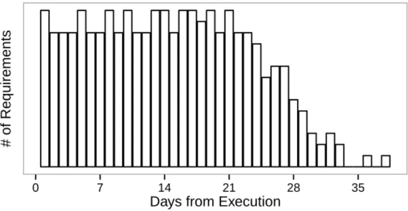
Figure 2-5: Hypothetical histogram of the number of requirements known based on the number of days until execution
0 7 14 21 28 35
Days from Execution
# of Requirements
schedule provides flight planners a convenient way to translate the baseline schedule into executable missions based on necessary lead times.
The value of optimization is the ability to schedule many requirements at once while taking advantage of synergies in requirement data. If there were no uncertainty in demand, we would use all known requirement data to solve the optimization model. Because there is uncertainty in demand, we must determine which requirements to include. Figure 2-5 presents a possible histogram showing the number of requirements known to the flight planners with the number of days until their execution. We must balance the value of using requirement data to create efficient routes with the cost of replanning if the data changes. For example, using the probability function in Figure 2-4 it might make sense to use the requirement data for those executing in the next ten days and ignoring the other requirement data because those requirements are likely to change. In addition, including more requirements makes it more difficult to solve the optimization model computationally.
2.3.1
Problem Definition and Assumptions
We refer to the problem of creating a schedule based on airlift requirement data as the military airlift scheduling problem. The goal of the military airlift scheduling problem is to assign aircraft capacity to routes in order to meet demand at minimum cost. Therefore, the output of our optimization model will consist of the number of aircraft assigned to each route, the sequence of stops along the route, the departure time at each stop along the route, and the amount of all requirements assigned to each route. The key aspects of the military airlift scheduling problem are the network, demand, and resources.
2.3.1.1 Network
The airlift network consists of a series of interconnected aerial ports. Some of these ports are the locations for Air Force wings. A wing is the home location for a specific aircraft type. Each aircraft type has multiple wings and some ports may be home to multiple wings.
Aircraft land and take off at ports to (un)load cargo and refuel. We assume that the capacity for storing cargo at a port is infinite. Each ground activity requires a minimum amount of time depending on the aircraft type. The number of aircraft at each port is restricted by the number that port can service in terms of taxiing and parking space. These restrictions are known as maximum on ground (MOG) constraints. In addition, each port may only operate during certain hours. For simplicity, we assume each port is open 24 hours per day in this thesis. However, constraining the operating hours for ports would likely reduce the solution space as the number of feasible aircraft routes would be reduced.
The minimum travel time between ports depends on the aircraft type and we assume this is known from historical data. Intermediate stops are necessary to refuel when the distance between two ports exceeds an aircraft’s range. Aerial refueling is a possibility for cargo aircraft making their effective range global. However, we do not consider aerial refueling to limit the size of the solution space and create a more tractable problem. Instead, we leave aerial refuelings as an option for flight planners to add to the baseline schedule created by the optimization model to shape it into an executable schedule with flexibility to withstand possible changes.
2.3.1.2 Requirements
Customer demand in the airlift scheduling setting is referred to as a requirement. Each requirement specifies a POE and POD in the airlift network as well as time restrictions. We assume a requirement stipulates an available to load date (ALD) at the POE and an earliest arrival date (EAD) and latest arrival date (LAD) at the POD. In addition, each requirement specifies the quantity and type of cargo to be transported.
In military airlift, cargo is described as either bulk, oversized, outsized, or passenger. Bulk cargo fits on a standard 463L pallet (104” x 84” x 96”) and can be transported on any cargo aircraft type. Oversized cargo is a single item that exceeds the dimensions of a standard pallet, while outsized cargo is a single item that exceeds 1000” in length, 117” in width, and 105” in height [3]. A cargo type, therefore, is any cargo with the same dimensions and weight. A requirement could demand multiple cargo types. We refer to a requirement-cargo type pair as a commodity. For example, an AH-64 Apache helicopter and a M1 Abrams tank are both described as outsized cargo, but each has distinct weight and dimensions. As a result, they are distinct commodities. Oversized and outsized cargo can only be transported on certain aircraft depending on their dimensions.
aircraft capacity depends on the total number of passengers, the total weight measured in short tons (stons), and the total footprint (area) measured in pallet positions. For example, an aircraft transporting tank treads is likely to run out of weight capacity before footprint capacity while an aircraft transporting helicopters is likely to run out of footprint capacity before weight capacity. As a result, we assume flight planners are able to translate requirement cargo data to commodities each with a weight and footprint.
Certain commodities can be classified as hazardous material, like ammunition and explosives. Flight planners must ensure that all cargo onboard an aircraft is compatible. We assume we know whether every pair of requirements are compatible to be onboard an aircraft simultaneously.
2.3.1.3 Aircraft and Aircrew
Aircraft and aircrew are the resources that carry out the airlift missions. Because we are not considering aerial refuelings, the relevant aircraft types include the C-130, C-17, and C-5. Each aircraft type has a specific cargo capacity and range. The capacity is in terms of passengers, weight in stons, and footprint in pallet positions.
Each AMC wing allocates a certain number of its aircraft on a daily basis for mobility purposes while reserving the rest for other uses including training. As a result, the number of aircraft assigned to a route on a specific day must be less than the number allocated. In addition, each aircraft must return to its home wing at the end of its route.
There are two types of aircrew. A basic aircrew is the minimum aircrew required and an aug-mented aircrew is a combination of two basic crews. There are two types of restrictions on an aircrew. An aircrew is limited to the number of working hours including ground activities by the crew duty day. An aircrew must take the minimum rest time called crew rest at a port to reset their crew duty day. An augmented crew extends the maximum crew duty day of a basic crew. Furthermore, aircrew tend to stay with the same aircraft throughout the route. In this thesis, we assume all aircrews are augmented and that we are limited by available aircraft.
2.4
Literature Review
We introduce the general approaches to solving problems similar to the military airlift scheduling problem in this section and further discuss their applications in the relevant chapters. In addition, we compare the military airlift scheduling problem to the scheduling problem airlines typically encounter. We finish by describing solution approaches (in the literature) for variants of the military airlift scheduling problem.
2.4.1
The Network Design Problem
The network design problem arises in many applications like transportation and communications. Magnanti and Wong (1984) describe the general network design problem and survey the variations and solution approaches in the literature. The network design problem is applicable in making strategic decisions like fleet acquisitions as well as tactical decisions like scheduling the effective use of the fleet similar to the military airlift scheduling problem.
In the network design problem, there are two types of decisions to be made. The design decisions assign capacity to edges in the network and the operating decisions assign commodities to those edges facilitating the necessary commodity flow. The objective then is to minimize the fixed cost of the design decisions and the variable cost of the operational decisions. The general network design problem includes the classic conservation of flow constraints as well as constraints that couple the design and operational decisions ensuring commodities only flow on the capacity assigned to each arc. The general network design problem assumes the operational decisions are continuous which is not the case in the military airlift scheduling problem because the types of cargo cannot be split arbitrarily.
The general network design problem can be formulated as a multicommodity flow problem where each commodity has a given origin and destination like the requirements in the military airlift scheduling problem. In addition, the military airlift scheduling problem is capacitated because there is not infinite aircraft capacity to transport requirements.
One of the successful optimization techniques to solve the network design problem uses Benders decomposition. One applies Benders decomposition iteratively by first setting the design variables to create a network, solving a routing problem to assign the operating decisions, and using the routing solution to create a new network. This solution provides a valid upper bound. After solving the routing problem, one adds Benders cuts that are inequalities representing the greatest improvement to the design problem based on the dual variables, which provides a valid lower bound. This process iterates until the gap between the upper and lower bounds is within some tolerance threshold.
There are numerous applications of the network design problem in the literature, especially in transportation. We discuss a few of these and relate them to the military airlift scheduling problem in Section 3.1.
2.4.2
The Pickup and Delivery Problem
There has been a considerable amount of work done on the pickup and delivery problem in recent years. Savelsbergh and Sol (1995) present a general pickup and delivery problem (GPDP) model that can be applied to many complex problems in practice, and provide a survey of the special cases of the general problem and solution approaches for each of these. In the GPDP, a set of vehicles,
each with a given start and end location and capacity, must satisfy a set of transportation requests, each with a given start and end location and load size. In addition, each request must be transported by a single vehicle without transshipment at intermediate locations. The objective of the GPDP is to determine the minimum cost pickup and delivery plan made up of multiple pickup and delivery routes.
There are three special cases of the GPDP in the literature: the pickup and delivery problem (PDP), the dial-a-ride problem (DARP), and the vehicle routing problem (VRP). In the PDP, all vehicles depart from and return to a central depot. The DARP is a PDP in which the requests represent people so every load size is one. The VRP is a PDP in which either all of the requests’ origins or destinations are located at the depot. The military airlift scheduling problem is best described as a PDP with multiple depots.
Transportation requests can be characterized as either static or dynamic. In the static case, all transportation requests are known prior to making the routes. In contrast, in the dynamic case, some requests are not known until during execution. As a result, one or more routes must be adjusted to serve the new requests. Savelsbergh and Sol (1995) note that dynamic problems are often solved as a sequence of static problems in practice. The military airlift scheduling problem is a dynamic problem and we propose solving a sequence of static problems.
Many practical applications of the PDP have constraints related to time. The pickup and delivery problem with time windows (PDPTW) is one in which the service at a location must occur in a given time window. In many practical applications, there are multiple time windows at each location because service can only occur during normal operating hours. In the military airlift scheduling problem, service at a pickup location must occur on or after ALD and the service at the delivery location must occur between EAD and LAD; furthermore, many airports do not operate 24 hours per day creating multiple time windows at each location.
In Section 4.1, we relate solution approaches to the PDP in the literature to the military airlift scheduling problem.
2.4.3
Airlines
Optimization has been applied with much success in the airline industry. In general, the airlines solve a series of optimization models sequentially to design the network, assign the fleet to the network, and assign crew to flights for planning purposes months ahead of execution. In execution, they rely on different strategies to adapt the optimal schedules in case of irregular operations.
Barnhart, Belobaba, and Odoni (2003) highlight the successful use of operations research tech-niques in various air transportation planning areas and address areas for future research. However, there are a number of differences between the military airlift scheduling problem and airline schedul-ing. First, airlines create their schedules well in advance of execution. They rely on forecasts and
simulate demand to test alternative network designs. Second, airlines typically create a schedule for each day of the week that repeats weekly. Finally, crew are able to swap between aircraft to allow greater utilization of aircraft.
The airline scheduling problem is usually treated as deterministic because it is large and complex. Optimal schedules make efficient use of aircraft which often leads to less slack in the schedule. In execution, this reduced slack could create significant increased cost in the event of changes or delays. Recently, there has been an effort to create schedules that are robust to these changes. Ahmadbeygi, Cohn, and Lapp (2009) and Lan, Clarke, and Barnhart (2006) present a strategy to reduce the realized cost of a schedule without increasing the planned cost by re-allocating scheduled slack to areas most prone to delay. This type of robust planning has potential to apply to the military airlift scheduling problem, but it is unclear whether it would be as successful because flight segments in military airlift schedules are not interconnected like airline schedules. Aircrew and cargo stay with the same aircraft eliminating the delay from propogating to other routes.
Optimal schedules are rarely executed in practice because of disruptions like weather and main-tenance. As a result, there has been considerable research focused on schedule recovery in the literature. Similar to planning, airlines often take a sequential approach by first recovering aircraft, followed by crew, and finally recovering passenger itineraries [6]. Airline controllers can swap air-craft or cancel/delay flights in order to minimize disruption. The difficulty in schedule recovery is the need for solutions quickly. The XOC directorate in the TACC manage schedule recovery in the airlift network. While we are not explicitly trying to account for schedule recovery, we attempt to create a schedule that lends itself well to managing disruptions.
2.4.4
Related Efforts
The military airlift scheduling problem is not new. Research on military airlift problems have been underway for several decades [15, 33]. We provide an overview of a few of the recent efforts.
Scheduling AMC channel missions distributing sustainment cargo is most similar to commercial supply chain networks. Nielsen, Armacost, Barnhart, and Kolitz (2004) utilize composite variables to design the AMC channel network. Composite variables combine different variable types (aircraft flow and cargo flow) into a single aircraft route variable that implicitly captures the feasible cargo flow. The result is an equivalent formulation that is computationally superior because it yields a tighter LP-IP gap. Channel missions occur when there is enough cargo to warrant an aircraft or enough time passes requiring new supplies. As a result, a channel mission utilizes a full or partial aircraft. The cargo for contingency and SAAM missions, on the other hand, can utilize multiple aircraft. Therefore, we would rather model cargo flow explicitly to allow the optimization to decide how best to split cargo between routes.
address this issue by developing a tool called the AMC allocator to aid the XOB in continuously tasking aircraft to missions scheduled by the flight planners. In addition, the AMC allocator is able to combine missions to utilize non-productive flying time. When missions cannot feasibly be accomodated, the tool uses heuristics to assign higher priority missions while minimizing disrup-tions to missions currently scheduled. Our goal is to create a baseline schedule for the military airlift scheduling problem that aggregates requirement types and makes a single decision. The AMC alloactor is still essential to allow decision-makers to adapt the baseline schedule to create an exe-cutable schedule in the continuously executing and oversubscribed environment. Our objective is to provide a better baseline schedule for the AMC allocator.
Few efforts have considered uncertainty because of the size of the problem. Baker et al. (2012) formulate a stochastic mixed-integer linear programming model using Benders decomposition. This approach incorporates uncertainty by solving the routing problem on a series of random scenarios. The Benders cuts are weighted by the probability of each scenario happening. The goal of this formulation was to provide the TACC with a 30-day aircraft allocation plan that is robust to changes so as to reduce the number of commercial aircraft leased in the short-term for a much higher cost than leasing them ahead of time. This formulation estimates demand based on forecasts and models at a high level-time is discretized into days and crew rest is not taken into account. On the other hand, our goal is to assign aircraft and cargo to routes based on that allocation to reduce the number of commercial aircraft leased in the short-term. Our formulation uses actual demand and models ground activity, travel time, and crew rest to ensure a feasible solution. While these problems are highly related and depend on one another, they differ in the data and assumptions they use as well as the goal of the problem. As a result, they require distinct approaches.
Chapter 3
Arc-based Formulation
The military airlift scheduling problem can be formulated as a multicommodity flow problem over a dynamic network. The goal is to flow a set of commodities from their POEs, beginning at a given time across a network to their PODs, by a given time. We must decide how best to design the network over which the cargo will flow by assigning aircraft capacity to each arc as well as commodities to each arc. To further complicate this challenge, we must include the numerous constraints specific to the military airlift scheduling problem like crew rest and cargo compatibility.
We begin the chapter reviewing the relevant research in the literature in Section 3.1 and relate it to the military airlift scheduling problem. We introduce the time-expanded network in Section 3.2. In Section 3.3, we formulate the military airlift scheduling problem as a multicommodity flow problem. We conclude with a discussion of the formulation’s merits in Section 3.4.
3.1
Related Work
The military airlift scheduling problem is a network design problem in which both the design decisions and the operational decisions are integral. In particular, it is a multicommodity flow problem where we must couple the aircraft route decisions with the cargo flow decisions to ensure sufficient capacity. Kotnyek (2003) surveys dynamic network flows in the literature and provides a few solution approaches. Kotnyek defines a problem as dynamic if the input is constantly changing or the input is time-dependent but known in advance. The military airlift scheduling problem is dynamic because the input is constantly changing as discussed in Section 2.2.3.
Most solution methods in the literature reduce a dynamic problem to a static one. In practical applications, the solution methods discretize time to create a static network using a time-expanded graph. In a time-expanded graph, there is a copy of each node for every time step in the time horizon and the arcs are drawn between them to represent the traversal time. The challenge using time-expanded graphs is determining a reasonable time step in order to ensure computational tractability.
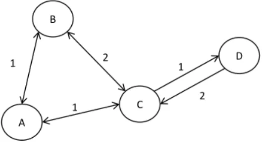
Figure 3-1: An example of a dynamic network where the labels on the arc represent travel times A B C D 2 1 1 1 2
The goal of any multicommodity flow problem is to satisfy the demands. There are many possible objectives to satisfy this goal. One can maximize total flow, minimize the time required to flow a given amount of commodities, minimize the cost to flow a given amount of commodities, or minimize the cost to flow the maximum flow. In the military airlift scheduling problem, we assume there is a cost for delivering a commodity late. We are interested in mimimizing the cost to design the network and the cost to flow all commodities from their source to their sink over this network.
Belobaba, Odoni, and Barnhart (2009) uses a variant of the expanded graph called a time-space network to solve the fleet assignment problem in the airlines. The time-time-space network includes a wrap-around arc for every node to ensure the balance of aircraft. For example, if an airport begins the day with five aircraft of a particular type, the wrap-around arcs ensure there are five of those type of aircraft at the location at the beginning of the next day. The military airlift scheduling problem is more constrained than this, however, because the aircraft not only have to be of the same type but also start and end at certain wing locations as well.
3.2
Time-expanded Network
The military airlift scheduling problem is dynamic because the input is constantly changing both in terms of requirement demand and the physical network. For example, the cargo for a requirement might double or the travel time between two ports might increase due to weather. We assume the input to our problem is known and unchanging. However, ignoring these uncertainties still results in a dynamic problem because the input is time-dependent. The travel time between ports is not instantaneous and requirements have time restrictions at the POE and POD. Figure 3-1 shows an example of a small dynamic network with the travel times labeled on each arc. In this example, port C is a hub connecting ports A and B with port D and the arcs are directed, meaning the travel time between ports depends on the direction.
We reduce our dynamic network to a static representation, similar to the literature, by employing a time-expanded graph. Figure 3-2 is the time-expanded version of Figure 3-1 over four time periods.
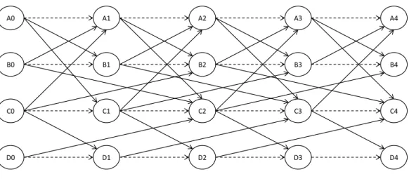
Figure 3-2: Time-expanded version of the network in Figure 3-1 A0 B0 C0 D0 A1 B1 C1 D1 A3 B3 C3 D3 A2 B2 C2 D2 A4 B4 C4 D4
We take travel time into account while constructing the network. As a result, the flow through an arc in the time-expanded version as instantaneous, resulting in a static network. The dashed lines represent ground arcs while the solid lines represent flight segments. Even in this small example with only four time periods, the number of arcs increased from 8 to 45. In general, the number of arcs leaving a node at each time period equals the number of ports within range of all aircraft plus an additional ground arc. The number of edges leaving a node is smaller near the end of the time horizon for arcs that require multiple time periods. For example, there are two arcs leaving port B in the dynamic network which results in three arcs leaving port B in each time period except for the last because the travel time from port B to port C is two time periods.
The goal of the military airlift scheduling problem is to create a baseline schedule that flight planners can implement immediately or adapt to create a more flexible schedule in case of changes. Therefore, we must discretize time with enough precision to capture accurate flight times and ground activities. In a continuous time setting, modeling exact times would lead to an intractable number of time periods. Thus, we must balance precision with performance. Published flight times are often estimated to the minute and ground activity times estimated to the nearest fifteen minutes. Discretizing a time period by fifteen minutes results in 96 time periods per day in the scheduling horizon. Because our scheduling horizon is likely to be ten to fourteen days, a more tractable discretization is a time period of an hour.
3.3
Arc-based Model
We formulate the military airlift scheduling problem using a time-expanded network with time periods {0, 1, . . . , T }. In this formulation, the design variables represent aircraft flow across the network while the operating variables represent the flow of cargo on the aircraft. Each aircraft
type has its own dynamic network and we transform each of these dynamic networks into one time-expanded network. As a result, each aircraft type has its own network defined over a subset of the time-expanded network.
We make some simplifying assumptions for this model. First, the ground activity time required at the next port is included in the traversal time. As a result, all flight arcs include the minimum ground time to (un)load an aircraft at the next port. Second, we do not model crew rest. Including these extra constraints would increase the size of the model because it would require modeling each individual aircraft. In addition, it would complicate the model because determining if crew rest is necessary depends on the crew’s current working time. A third simplification is to aggregate design variables by aircraft type. Aggregating in this way reduces the size of the problem significantly, but it means we cannot check individual aircraft capacity. It is possible to have enough capacity in aggregate, but not enough capacity for individual aircraft because our cargo cannot be split arbitrarily. Furthermore, we cannot ensure an aircraft returns to its home wing at the end of its route. Instead, we can only ensure there is the proper balance of aircraft by type at each wing similar to the airlines. These assumptions yield the problem of determining the optimal aircraft schedule, one similar to the airlines fleet assignment problem.
3.3.1
Sets
Requirements may consist of multiple cargo types (e.g., vehicle, pallet, passenger), and we refer to a requirement-cargo type pair as a commodity. The nodes in our network represent an airport at a specific time. The edges in our network represent either a flight segment or a ground segment. The sets we use in our model are the following:
• K = {1, 2, ..., |K|}: set of commodities; • N = {1, 2, ..., |N |}: set of nodes;
• W ing ⊆ N : subset of nodes that are wings; • M = {1, 2, . . . , |M |}: set of aircraft types;
• Km⊆ K: subset of commodities able to be transported on an aircraft type m;
• E = {1, 2, ..., |E|}: set of edges;
• F ⊆ E: subset of edges that are flight segments; • I(n) ⊆ E: subset of edges entering node n; and • O(n) ⊆ E: subset of edges leaving node n.
A commodity can either arrive at the POD by LAD, after LAD, or not at all. To allow any of these possibilities, we define the node, Sinkk∈ N , for every commodity k and artificial arcs with infinite capacity from the source node of the commodity, P OEk, to Sinkk and from the node associated
with the POD of the commodity at t = T to Sinkk. The commodity must arrive to the sink using
one of the artificial arcs. Commodity flow through the first artificial arc does not reach the POD at all and commodity flow through the second artificial arc reaches the POD. The node, Earlyk ∈ N ,
represents the kth commodity’s POD in the time period prior to EAD.
3.3.2
Parameters
The parameters we use in our model are the following: • Allocn: demand for aircraft at wing n;
• W CAPm: capacity of aircraft type m in weight (stons);
• V CAPm: capacity of aircraft type m in pallet positions;
• P CAPm: capacity of aircraft type m in passengers;
• M OGn: aircraft capacity of port n in number of aircraft parking spaces;
• qm: number of aircraft parking spaces required for aircraft type m;
• Dk: demand for commodity k in quantity (number of items);
• ωk: weight of commodity k in stons;
• νk: footprint of commodity k in pallet positions;
• Cm
e : fixed cost of aircraft type m flying edge e;
• Wk,m
e : variable cost of transporting cargo of commodity k on aircraft type m on edge e; and
• δm e =
1, if edge e is in the network of an aircraft of type m 0, otherwise
.
Each wing allocates the number of aircraft available each day. The node associated with a wing on the first time period each day will be a source if the number of allocated aircraft increases from the previous day. Similarly, the node associated with a wing on the last time period each day will be a sink if the number of allocated aircraft decreases from the previous day.
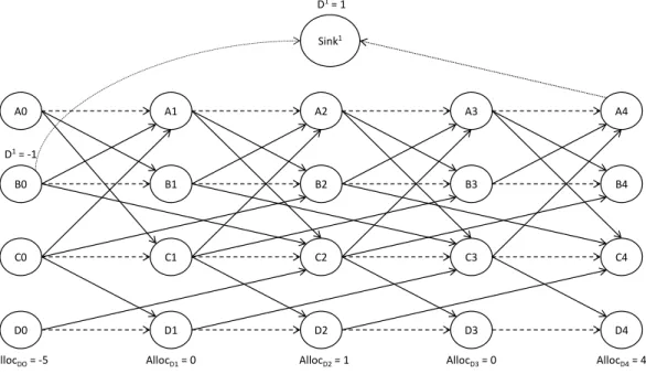
Figure 3-3 includes the sink node, Sink1, and artificial arcs, represented by the dotted lines, for
commodity 1. In this example, commodity 1 has a POE at port B with an ALD at the beginning of the first time period and a demand of one unit. Figure 3-3 also shows the supply and demand of
Figure 3-3: Time-expanded network with a sink node and artificial arcs for one commodity and one wing at port D A0 B0 C0 D0 A1 B1 C1 D1 A3 B3 C3 D3 A2 B2 C2 D2 A4 B4 C4 D4 Sink1 D1 = -1 AllocDO = -5 D1 = 1 AllocD4 = 4
AllocD1 = 0 AllocD2 = 1 AllocD3 = 0
aircraft for the wing at port D. It supplies five aircraft at the beginning of the first period, demands an aircraft at the end of the second, and demands the remaining four aircraft at the end of the final time period.
We include in the variable cost for transporting cargo on an edge a per unit penalty for either delivering a commodity late or not at all. In this way, the penalty for delivering a commodity depends on the time of delivery and the type of commodity.
3.3.3
Decision Variables
We have two sets of decision variables: • xm
e =number of aircraft of type m assigned to edge e; and
• yk,m
e = number of items of commodity k assigned to aircraft type m on edge e.
3.3.4
Formulation
We formulate our model in the following way:
min xn e,yke X m∈M X e∈F Cemδme xme + X m∈M X k∈K X e∈E Wek,myek,m (3.1)
s.t. X e∈I(n) δemxme − X e∈O(n) δemxme = Allocn ∀n ∈ W ing, m ∈ M 0 ∀n ∈ N \ W ing, m ∈ M (3.2) X e∈I(n) yek,m− X e∈O(n) yek,m= −Dk ∀k ∈ K, m ∈ M, n = P OEk 0 ∀k ∈ K, m ∈ M, n ∈ N \ P OEk∪ Sinkk Dk ∀k ∈ K, m ∈ M, n = Sinkk (3.3) X m∈M X e∈I(Earlyk) yek,m= 0 ∀k ∈ K (3.4) X m∈M X e∈I(n) qmδemxme ≤ M OGn, ∀n ∈ N (3.5) X k∈Km ωkyek,m≤ W CAPmδm e x m e, ∀e ∈ F, m ∈ M (3.6) X k∈Km νkyk,me ≤ V CAPmδemxme, ∀e ∈ F, m ∈ M (3.7) X k∈Km yek,m≤ P CAPmδm e x m e, ∀e ∈ F, m ∈ M (3.8) xme , yk,me ∈ Z+ ∀e ∈ E, k ∈ K, m ∈ M (3.9)
Our objective is to minimize the fixed cost of assigning an aircraft to a flight segment and the variable cost (including penalty costs for late cargo) of transporting cargo on a flight segment. Constraints (3.2) conserve the flow of aircraft, ensuring aircraft are supplied and demanded where appropriate. Similarly, constraints (3.3) conserve the flow of each commodity from its source, P OEk, to its sink, Sinkk, ensuring that it does not leave its POE until ALD and it enters the sink node
through one of the artificial arcs (allowing the commodity to arrive at the POD on time, late, or not at all). We ensure a commodity does not arrive prior to its EAD in constraints (3.4) and that there are not more aircraft at a port at any time than there is capacity in constraints (3.5). We couple aircraft and cargo flow together by ensuring there is enough aggregate aircraft capacity for each aircraft type on every flight segment in constraints (3.6)-(3.8). Finally, constraints (3.9) restrict aircraft and commodity flow to be non-negative integers.
3.4
Summary
Modeling the military airlift scheduling problem using a time-expanded network is natural. It is intuitive to interpret the flow of aircraft and cargo over the time-expanded network. The suitability of this formulation, however, is not practical because of the simplifying assumptions and the size.
We make several simplifying assumptions to formulate the military airlift scheduling problem similar to an airline fleet assignment problem. Scheduling aircraft and crew separately and removing ownership of an aircraft from a wing would require AMC to institute significant changes to their business process. Furthermore, it is not clear that these simplifying assumptions would yield a model that is tractable in realistic-sized instances.
AMC operates a global network that results in a large time-expanded network. Estimating the size of the network is challenging because military aircraft can utilize commercial airports and not all military bases have an airfield. We use the number of large or medium (replacement value of $915M or greater) DOD sites to estimate the number of ports in the network. At the start of FY12, the DOD controlled 257 large or medium sites around the world [12]. This does not include the 4,444 small sites or commercial airports AMC aircraft may utilize, so assuming a dynamic network of 257 nodes is reasonable. Assuming T = 240 (discretizing time per hour for ten days), this results in a time-expanded network of 6,168 nodes. Assuming that each aircraft type can reach ten airports from any given airport, this results in a dynamic network of 2,570 flight segments for each aircraft type. The time-expanded network results in approximately 1,850,400 edges (i.e. the number of xm e
decision variables). Even a rougher discretization of time to time steps of six hours results in over 300,000 edges.
The global nature of the AMC air network makes solving the military airlift scheduling problem challenging. Furthermore, our problem requires an integral solution because aircraft and cargo cannot be split arbitrarily. Kotnyek (2003) points out that the integral multicommodity problem is not solveable in polynomial time . Therfore, we must reformulate to yield a more tractable model while incorporating the constraints characteristic of the problem.
Chapter 4
Route-based Formulation
Solving the military airlift scheduling problem using traditional network optimization is not tractable due to its size and characteristics as discussed in Section 3.4. Instead, we reformulate the problem as a route-based optimization model and develop column generation techniques to address it.
In our reformulation, the decision variables correspond to aircraft routes. We build feasible aircraft routes in steps separate from solving the optimization model. By ensuring that routes we build are feasible with respect to travel time, ground time, crew rest, and requirement restrictions, we do not need to encode these characteristics within the optimization model, thus reducing the number of constraints. Further, we reduce the number of decision variables by generating only a fraction of feasible aircraft routes.
The remainder of the chapter is organized as follows. In Section 4.1, we give a brief review of related work in the literature. In Section 4.2, we explain our route generation algorithm and illustrate with simple examples. In Section 4.3, we detail our Route-based optimization model. We explain our two column generation approaches in Section 4.4. Finally, we finish in Section 4.5 with an alternative optimization model that incorporates departure time flexibility.
4.1
Related Work
4.1.1
The Pickup and Delivery Problem
In Section 2.4.2 we introduced the PDPTW and provided the general framework. Numerous efforts have formulated the PDPTW using a column generation approach on a set partitioning problem. Cordeau and Ropke (1990) provide a branch and cut algorithm to solve the set partitioning problem to optimality while Arunapuram et al. (2003) use dynamic programming to solve their problem to global optimality. These solution techniques do not work on the large-scale problems characterized by our application. Much research has focused on heuristic methods to generate feasible vehicle