HAL Id: hal-01024270
https://hal.archives-ouvertes.fr/hal-01024270
Preprint submitted on 15 Jul 2014
HAL is a multi-disciplinary open access
archive for the deposit and dissemination of
sci-entific research documents, whether they are
pub-lished or not. The documents may come from
teaching and research institutions in France or
L’archive ouverte pluridisciplinaire HAL, est
destinée au dépôt et à la diffusion de documents
scientifiques de niveau recherche, publiés ou non,
émanant des établissements d’enseignement et de
recherche français ou étrangers, des laboratoires
A Reduction Algorithm for Packing Problems
Michaël Gabay, Hadrien Cambazard, Yohann Benchetrit
To cite this version:
Michaël Gabay, Hadrien Cambazard, Yohann Benchetrit. A Reduction Algorithm for Packing
Prob-lems. 2014. �hal-01024270�
A Reduction Algorithm for Packing Problems
Michaël Gabay
∗, Hadrien Cambazard
∗, Yohann Benchetrit
∗July 15, 2014
Abstract: We present a reduction algorithm for packing problems. This reduction is very generic and can be applied to almost any packing problem such as bin packing, multi-dimensional bin packing, vector bin packing (with or without heterogeneous bins), etc. It is based on a domi-nance applied in the compatibility graph of a partial solution and can be computed in polynomial time in the input size and the number of bins, even on instances with high-multiplicity encoding of the input.
Keywords: Packing, Reduction algorithm, Multi-dimensional Packing, Vector Packing, Bin Packing, High-Multiplicity
1
Introduction
We are interested in combinatorial packing problems in general. There are usually two ways to solve such problems. The first one is to focus on the assignment of the items: one has to decide in which bin each item will be packed. The second one is focused on patterns: given all the feasible packings of items in bins, which patterns are used in an optimum solution and how many times? This second approach is the generalization of [1] approach for the cutting-stock problem. Pattern based exact algorithms are usually more efficient when the number of patterns is limited or there are items with large multiplicities while assignment based algorithms are usually better for heuristics and when the number of different items is large.
In this paper, we focus on assignment based approaches and propose a reduction algorithm based on a dominance property. In an assignment based solver for a packing problem, this prop-erty can be used to fix the assignment of many items at once and reduce the problem to a smaller packing problem. This is especially well suited to be integrated in branch-and-bound approaches for packing problems.
In packing problems, Dual Feasible Functions have been extensively used to obtain lower bounds [2, 3]. In this paper, we are interested in reduction procedures which ensure that op-timality is preserved in the reduced problem. Such reductions have already been proposed by authors on specific packing problems, see e.g. [4–6]. [6] introduced the notion of Identically Fea-sible Function (IFF) to properly state the idea of reductions. The authors then propose IFF for 2-dimensional bin packing problems to remove small items and increase the size of large items. In [7], they investigate the use of tree-decomposition techniques to identify subproblems to be solved independently in a 2-dimensional packing problem with conflicts. Notice that reductions procedures or problem separation techniques were proposed very early by [4].
Reduction algorithms are often critical for the success of packing algorithms, see e.g. [8,9] for presentation of reduction algorithms on the knapsack and the bin packing problems. In multi-dimension or with additional constraints, it is even more critical to be able to reduce packing problems to the smallest possible core problems. In this paper, we present a reduction algorithm
which can be used on whole instances of packing problems and can also be applied in the course of an assignment based algorithm for packing problems.
2
Definitions
We define a pure packing problem as a packing problem in which the capacities of the bins and the weights of the items are non-negative and the only constraints are the capacity constraints. The results presented in this paper are however much more general than this case. A number of other constraints can be added to the problem and if we simply take them into account when we compute the compatibility graph, then all the results for pure packing problems will still hold. For instance, we can add the following types of constraints:
• Variable item weights: if the weights of an item depends on the bin it is assigned to.
• Conflict constraints between items: if there are sets of conflicting items such that two items in a same set cannot be in a same bin.
• Incompatibility constraints between items and bins: if some items are incompatible with some bins, for instance because the items are fragile or heavy.
Basically, the results can be generalized to most constraints which do not involve both set of bins and set of items (for instance, spread or dependency constraints involve both set of bins and set of items).
A partial solution of a packing problem is a solution in which some but not all the items have been packed. Given a partial solution of a packing problem, observe that packing the remaining items is an instance of the same packing problem but in which bins have variable sizes. Pure packing problems have the nice property that for any feasible assignment, any subset of the bins and of the items in these bins is a partial solution of this problem and a feasible solution to the packing problem defined by only these bins and items. So if a partial solution is not feasible, then there is no feasible solution of the whole instance having this partial solution as a subset.
This is not necessarily true for “non-pure” packing problems such as the Machine Reassign-ment Problem1. In this problem, we also have to spread the items: a subset of a feasible solution may violate the spread constraint. However, the partial solution property holds for the underlying vector bin packing problem with heterogeneous bins.
We say that a partial solution P is feasible if it is a feasible solution to the pure packing problem defined with only the bins and items appearing in P. We say that it is g-feasible (g stands for globally) if P is a subset of a feasible solution to the underlying pure packing problem. Given a bin b (resp. a subset of bins X) we denote by bP(resp. XP) the set of items contained within this
bin (resp. this subset of bins) in partial solution P.
Given a feasible partial solution, in the remaining subproblem, not all items fit into all bins. Let b be a bin, we say that an item i < bPis compatible with or fits into the bin b if the set of items
bP∪ {i} fits into the bin b (starting from P, packing i into b gives another feasible partial solution).
Let I be the set of items and B be the set of bins. In a partial solution P, we denote by IP the
set of unpacked items and by BPthe set of bins in which at least one item from IPfits. Let X ⊆ BP
be a subset of bins, we denote by Γ(X) = {i ∈ IP: ∃b ∈ X s.t. i fits into b}, the set of items which are
compatible with these bins.
We have the following property:
Property 1. Given a partial solution (possibly with no item assigned) P, for any X ⊆ BPsuch that there
is a feasible packing of Γ(X) into X, let PX be a partial feasible solution extending P and in which all
items from Γ(X) are assigned to X. P is g-feasible if and only if PXis g-feasible.
Proof. If PXis g-feasible, since P is a subset of PX, P is obviously g-feasible.
Suppose P is g-feasible and consider a feasible solution S (S is a solution to the complete pure packing problem) which is an extension of P. Notice that bins from X contain only the items which they were assigned in P and some items from Γ(X). If we remove the items in Γ(X) from S, we obtain a partial solution P′ which is clearly g-feasible. Moreover, in P′, the bins from X are assigned exactly the same items as in P. So packing Γ(X) into X is feasible in P′. We pack these items as in PXand obtain a feasible solution S′containing PX. Therefore, PXis g-feasible.
Property1gives a decomposition of packing problems into subproblems. It states that if we can find a subset of bins such that there is a feasible assignment of all of their compatible items within these bins, then we can pack these items in the bins and remove both the bins and items from further considerations. A valid set X is illustrated Figure1, page5.
Hence, if we can find such a set of bins and a feasible packing, we can assign all of them at once and reduce the problem to a smaller subproblem. However, given a set, determining whether it verifies the property is a hard matter. For instance, for X = B and P = ∅ we have the initial packing problem and even the (single dimension) bin packing problem is strongly N P -hard and does not have a PTAS (unless P = N P of course).
We propose a reduction algorithm based on flow-computation in the graph of items and bins compatibilities. Given a partial or an empty solution, it finds a feasible set X and a feasible assign-ment of the items from Γ(X) into X. In Section5, we present the reduction algorithm with single item assignments. It also proves that any packing problem in which the number of bins is greater than or equal to the number of items can be reduced in polynomial time to a packing problem with fewer bins than items. In Section6, by using network flows, we generalize the results of Sec-tion 5to more complex assignments. We present preliminary results and additional definitions in Section 4. In the next section, we expose a quick discussion explaining complexity matters in these problems and why the results presented in this paper are holding for both decision and optimization packing problems.
3
Discussion
We have not stated yet whether we are considering decision or optimization problems and which are the complexity parameters. In this section, we seek to clarify these matters.
3.1
Decision or Optimization ?
The problem description may let the reader think that we are focusing on decision problems. In decision problems, the number of bins is given. So checking bins’ and items’ compatibilities is straightforward. Moreover, we do not have to consider adding or removing bins: B is known in advance. In our case, we are considering both decision and optimization problems. In optimiza-tion problems, in any assignment based algorithm, if an item does not fit in any bin, then we have to add a new bin (the partial solution is not g-feasible with the current number of bins). So we can modify the algorithm to immediately add a new bin and extend B with it once an item is compatible with none of the bins. The results of the dominance properties and the reductions applied are not modified since adding a bin neither adds nor removes any edge from the other bins. One can argue that there are maybe several types of bins but, in this case, in exact algorithms we “only” have to branch to select which kind of bin is added. The algorithm can be adapted by simply branching earlier on the new bins. Moreover, in order to minimize the number of bins, many algorithms repeatedly solve the problem with a fixed number of bin. In this case, we are actually solving several decision problems.
In the following, we assume that the number of bins is fixed and equal to |B| but the results can easily be generalized to optimization problems.
3.2
Complexity
Regarding complexity, the algorithm is polynomial in the input size and in |B|. If we have a high-multiplicity encoding of the input, it is legitimate to expect a high-multiplicity encoding of the output. For instance an output can be specified by giving the patterns used (each pattern being a way to fill a bin) and for each pattern how many items of each type are contained in the bin and how many times the pattern is used. Such an encoding is compact but not necessarily polynomial in the input size. Indeed, |B| is not necessarily polynomial in the input size when a high-multiplicity encoding is used. However, we are interested in algorithms here (and in solving N P -hard problems. . . ) and, above all, we are considering assignment based algorithms. Meaning that |B| is small enough to consider such approaches. Finally, observe that even assignment based algorithms can assign many items at once.
In the end, the algorithm may not be polynomial in the input size but it is polynomial in the size of the space which the programmer decided to allocate to his algorithm.
In the following, we assume that given a partial solution P, an item i and a bin b, we have access to an oracle which tells us whether i fits into b. However, we remark that for hyper-boxes geometric packing problems (strip packing, multi-dimensional bin packing,...) this problem is N P -hard. Yet, for algorithms which do not consider reorganizing the contents of the bins in partial solutions, we can usually find out in polynomial time whether an item fits into a given bin.
4
Preliminaries
In the following, we use the bipartite compatibility graph of partial assignments. In this graph, each unpacked item is a vertex in the first partition and each bin in which at least one item fits is a vertex in the second partition. We denote this graph by GP = (IP, BP, EP); the set of vertices is
denoted by VP= IP∪BP. Let u ∈ IPand v ∈ BP, the edge {u, v} is in EPif the item u fits into the bin
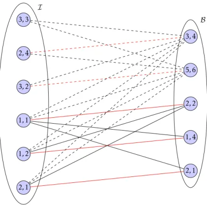
v. Figure1illustrates the compatibility graph of a vector packing problem with two dimensions and also gives a set X satisfying Property 1. We remark that if we use constraint programming, the compatibility graph is obtained directly from the variables domains after filtering.
In a graph G = (V , E), we denote by δ(u) = {{u, v} : v ∈ V and {u, v} ∈ E} the set of edges incident to u ∈ V ; we denote by d(u) = |δ(u)| the degree of a vertex u ∈ V and by Γ(X) = {v ∈ V \ X : ∃u ∈ X s.t. {u, v} ∈ E} the neighbors of a set of vertices X ⊆ V . For singletons, we use Γ(v) instead of Γ({v}). In the following we will also use directed graphs but d, δ and Γ always refer to the (underlying) undirected graph.
In the next section, we use Hall’s theorem which is recalled below:
Theorem 1(Hall’s Theorem). A bipartite graph G = (U, V , E) has a matching saturating U if and only
if ∀X ⊆ U, |X| ≤ |Γ(X)|.
Now, let us consider the compatibility graph GPfor a given P and derive some basic properties
from this graph. Let u ∈ IP, if d(u) = 0 then the item u cannot be packed. Hence, the partial
solution P is g-infeasible. If d(u) = 1, then δ(u) = {{u, v}} for some v ∈ BPand if the number of bins
cannot be increased, the item u has to be packed into the bin v.
We said that we are only interested in bins in which at least one of the remaining item fits. Notice that if we added the other bins to the graph their degrees would be 0 so they would be isolated vertices which are modeling nothing useful. For a bin v ∈ BP, if d(v) = 1 then only one
item u ∈ IPcan be assigned to the bin v. In any pure packing problem, it is dominant to pack this
item into v. So we can assign item u to v and remove u and v from the compatibility graph. Observe that, when an item is assigned to a bin, we can update the compatibility graph and ensure that all degrees are greater than or equal to 2 in linear time in the size of IP. When the
I B 3, 3 2, 4 3, 2 1, 1 1, 2 2, 1 3, 4 5, 6 2, 2 1, 4 2, 1
The labels in the vertices from I are the requirements of the items in each dimension and the labels in the vertices from B are the remaining capacities of the bins in each dimension. Edges are denoting compatibilities. The three vertices {(2, 2), (1, 4), (2, 1)} from B form a set X satisfying Property1. Plain edges are edges from δ(X), other edges are dashed. A maximum matching in this graph is given in red.
Figure 1: The bipartite compatibility graph of a vector packing problem.
we do not assume that all degrees are greater than 1 since it can result in loss of generality for optimization problems (when an item u is assigned because d(u) = 1).
We first present the reduction when there are no multiplicities on the items and at most one item is assigned to a bin. Then, we generalize the reduction algorithm to account for multiplicites on the items and perform reductions with assignments of more than one item into a bin. In this general case, the compatibility graph will be slightly different. We present the changes in Sec-tion6.
5
Matching-based reduction algorithm
In this section, we show that given the compatibility graph we can find a set X satisfying Property1
and which is maximum for one-to-one assignments. A one-to-one assignment is an assignment in which each item is assigned to one bin and at most one item is assigned to a bin.
In order to find this set, we compute a maximum matching M ⊆ EP in the compatibility
graph GP. We orient the edges from GPas follows: let u ∈ IPand v ∈ BPtwo adjacent vertices, i.e.
e= {u, v} ∈ EP, if e ∈ M we orient e from v to u, otherwise e is oriented from u to v. We denote by
DM= (IP, BP, AM) the new directed graph. Let UMbe the set of all vertices from IPwhich are not
saturated by M, we denote by RMthe set of vertices reachable from UMin DM(we have UM⊆ RM),
and by KM= IP\ RMthe items which are unreachable from UMand LM= BP\ RMthe bins which
obtained from the matching Figure1. We have the following result:
Theorem 2. LM= BP\RMis a set satisfying Property1and the matching M gives a feasible assignment
of Γ(LM) into LM. RM∩ I RM∩ B KM LM 3, 3 2, 4 3, 2 1, 1 1, 2 2, 1 3, 4 5, 6 2, 2 1, 4 2, 1
The oriented graph corresponding to the example and the matching illustrated Figure2. The vertices are labeled as in Figure2. The gray vertex (3, 3) is the only node in the set UM. All dashed edges are oriented from left to right and all red
edges are edges from the matching and oriented from the right to the left.
Figure 2: An oriented compatibility graph
Proof. This proof is based on the proof from König’s theorem [10]. König’s theorem states that in a
bipartite graph, the cardinality of a maximum matching is equal to the cardinality of a minimum vertex cover.
If M saturates IP, then UM = RM = ∅ and LM = BP. Moreover, assigning each item to its
corresponding bin in the matching is clearly a feasible assignment of all items.
Otherwise, M does not saturate IP. By definition of RM, there is no arc from RMto LM.
More-over, there is no arc from LMto RMsince any vertex from RM∩ IPis either not saturated by M (in
UM) or matched with a vertex in RM∩ BP. So Γ(LM) ⊆ KM.
Finally, by definition of UM and KM, all vertices in KM are saturated by M. Moreover, let
u ∈ IP and let e = {u, v} ∈ M if v ∈ RM, then by definition of RM, u ∈ RM. Hence, the matching
M saturates all vertices of KM using edges from BP\ RM = LM to KM. Therefore KM ⊆ Γ(LM)
and hence Γ(LM) = KM. Moreover, assigning each item from KM to its corresponding bin in the
matching is feasible since only one item is assigned to each bin and edges are denoting feasible assignments.
Based on Theorem2, we can compute a feasible set X of one-to-one assignments using Algo-rithm1.
Compute a maximum matching M in GP;
Compute RM;
return M, X = BP\ RM; // The matching gives the assignment
Algorithm 1: Matching-based reduction algorithm
The reduction assigns any item in KM to its bin matched by M. Then, LM and KM are taken
out of consideration. We denote by P′ the new partial assignment. If KM was empty, then P′= P.
We have the following property:
Property 2. The set X returned by Algorithm1is maximum for one-to-one assignments.
Proof. Let Q ∈ BP be a feasible set for Property 1with one-to-one assignments. Observe that a
one-to-one assignment is an assignment of one item into each bin, so it is a matching. Since Q is a feasible set, there is a one-to-one assignment, hence a matching, of Γ(Q) into Q. Let W be a second feasible set for Property 1with one-to-one assignments. Clearly, there is a matching saturating vertices from Γ(W ) with edges from Γ(W ) to W . Hence, there is a matching saturating vertices from Γ(W ∪ Q) with edges from Γ(W ∪ Q) to W ∪ Q and |Γ(W ∪ Q)| ≤ |W ∪ Q|.
Therefore, in order to show that a feasible set X with one-to-one assignments is maximum, it is sufficient to show that it is maximal with respect to the union. Moreover, observe that for any set W ∈ BP, disjoint from Q, if Q ∪ W is a feasible set with one-to-one assignments, then there
is a matching saturating vertices from Γ(W ) \ Γ(Q) with edges from W to Γ(W ) \ Γ(Q). Hence, |W | ≥ |Γ(W ) \ Γ(Q)|. Therefore, it is sufficient to show that once the reduction has been applied, in the new compatibility graph there is no set X ⊆ BPsuch that |X| ≥ |Γ(X)|.
Once the reduction has been performed and items from KMhave been assigned to the bins from LM,
we denote by P′ the extended partial assignment and we have: Lemma 1. In GP′, ∀X ∈ BP′, |X| < |Γ(X)|.
Proof of Lemma1. Let M′be the restriction of M to GP′; M′is a maximum matching of GP′. Clearly,
M′is not a perfect matching and LM′= KM′= ∅.
Hence, the vertices of BP′ = RM′∩ BP′ are saturated by M′. By Hall’s theorem, ∀X ⊆ BP′,
|X| ≤ |Γ(X)|. Suppose there exists X ∈ BPsuch that |X| ≥ |Γ(X)|, then |X| = |Γ(X)| and X is saturated
by M′. Therefore, M′is a perfect matching of GP|X∪Γ(X)′ (the restriction of GP′to X ∪ Γ(X)). Hence,
Γ(X) ∩ UM′= ∅, there is no arc from BP′\ X into Γ(X) and obviously there is no arc from IP′\ Γ(X)
into X. Which contradicts LM′= ∅ and KM′= ∅.
By Lemma1, BP\ RM is maximal with respect to the union and hence, it is maximum for
one-to-one assignments.
As a consequence of Lemma 1, in a single run of the algorithm, we have proceeded to all feasible one-to-one assignments.
The algorithm computes a maximum matching and marks the vertices of the graph in a single pass. Therefore, the overall complexity is the complexity of the maximum matching algorithm which is O(|I |2.5) if we use Hopcroft-Karp’s matching algorithm [11].
A second consequence is the following:
Corollary 1. For pure packing problems in which we can compute the compatibility graph in polynomial time: any instance with more bins than items (|I | ≤ |B|) can be reduced to an instance with more items than bins (|I | > |B|) in polynomial time.
On consecutive runs of the algorithm, the efficiency of the maximum matching algorithm can be improved by updating the previously computed maximum matching and using it for a hot start of the matching algorithm.
Observe that for the special case of the pure bin packing problem finding the set X is trivial. Indeed, an item which fits into a bin fits into all bins with smaller weight. Hence, the compatibility graph is (doubly) convex. The maximum matching can be obtained by simply sorting the bins and the items, or even in linear time with the algorithm from [12].
6
Generalized reduction algorithm
In this section, we extend previous results to other assignments than one-to-one assignments and instances which are specified using a high-multiplicity encoding of the input.
First, observe that a matching in a bipartite graph G = (U, W , E) is an integer flow in the same graph extended with a source s connected to all vertices from U and a sink t connected to all vertices from W , and all edges from E being oriented from U to W . We now use this oriented compatibility graph D = (V , A) (resp. DP = (VP, AP)) in place of the previous one. We denote by
c(u, v) (resp. cP(u, v)) the capacity of the arc (u, v) in the compatibility graph (resp. the
compati-bility graph of the partial solution P).
In order to generalize the results to high-multiplicity, we need to ensure that the size of the graph is polynomial in the input size and |B|. In order to achieve this, we simply merge vertices from a same item type into a single vertex. Suppose that I is now the set of different item types and mithe multiplicity of item i ∈ I . In a partial solution P, we now consider that IPis the set of
remaining different item types and mPi denote the residual multiplicity of the item i (the number of items of type i which are not already packed in P). For an item i ∈ I , we set c(s, i) = mi (resp.
cP(s, i) = mPi ) and c(i, b) = +∞ ∀b ∈ B with (i, b) ∈ A.
Now, suppose you expand this graph and replicate mi times each vertex i ∈ I . Let b ∈ B and
N = {i ∈ I : (i, b) ∈ A} (since Γ is the neighborhood in the undirected graph, this is also Γ(b) ∩ I ). We denote by κbthe maximum number such that any subsets of items in N of size at most κbcan
be packed in b; κb= max{k : ∀J ⊆ N with |J| = k, J fits into b}. We call κbthe robust capacity of the
bin b. The capacity of the arc (b, t) is set to c(b, t) = κb. We denote by κ = (κ1, . . . , κ|B|) the vector of
robust capacities of the bins. We define κPb and capacities of the arcs similarly for partial solutions. Similarly to one-to-one assignments, we define a κ-assignment as an assignment in which at most
κbitems are assigned to the bin b.
The compatibility graph now looks like the graph Figure3. An example of a compatibility graph is illustrated Figure4.
u1 u2 u3 u4 v1 v2 v3 s t m1 m2 m3 m4 κ1 κ2 κ3
3, 4 2, 5 2, 2 1, 1 0, 4 0, 1 5, 5 2, 7 3, 3 0, 8 s t 1 1 1 3 1 2 1 1 2 3
Figure 4: An example of a generalized compatibility graph for a 2-dimensional vector packing problem
Observe that determining the values of κ is easy for single dimension bin packing problems: Sort the items by decreasing order of the weights and let r be the remaining space in bin b. Let wi
be the weight of item i and j = min{k :Pki=1miwi> r}. Then, κb=Pj−1i=1mi+ max{k : k ≤ mjand k ×
wj+P
j−1
i=1miwi≤ r}.
For vector bin packing problems, we compute κb by applying the same procedure on all
di-mensions: κb = min κjb where κjb is the value of κb for the bin packing problem on dimension
j.
For other packing problems, this problem can be N P -hard but as we will see, only the diversity of combinations is depending on the values of κ’s. So setting them to 1 will simply limit solutions to one-to-one assignments. Additionally, any heuristic giving a lower bound on the values of κ’s will yield feasible reductions. So, for instance, in a 2-dimensional bin packing problem, if we create a rectangle whose width is the largest width among the items compatible with b and whose height is the largest height among the items compatible with b; then any heuristic giving a feasible number of such rectangles which can be packed, gives a lower bound on κb. And we can set the
capacity c(b, t) to this lower bound.
Finally, we can use fixed-parameter tractability results: when the number of items is fixed, for a set of items of the given size, we can usually determine in polynomial time whether the items fit. One can use such results when the number of compatible items is small but the number of combinations of a fixed number of items is quickly impracticable if we consider combinations of more than 3 items and bins with many compatible items.
Algorithm2gives the generalized reduction algorithm.
The construction used for Algorithm1 is similar to the construction used in a proof from König’s theorem [10]. König’s theorem states that in a bipartite graph, the cardinality of a maxi-mum matching is equal to the cardinality of a minimaxi-mum vertex cover. Computing RMas we did in
Algo-Compute a maximum flow f in DP;
Compute Rf, the set of all vertices reachable from s in the flow residual graph;
return f, X = BP\ Rf; // The flow gives the assignment
Algorithm 2: Generalized reduction algorithm
rithm2, we compute the set of reachable vertices in the residual graph which is actually the same as computing a minimum cut based on a maximum flow. It is very natural to compute similar dual elements since König’s theorem is a special case of the max-flow min-cut theorem.
In Algorithm2, we mark R, the set of all vertices which can be reached from s in the residual graph. Clearly, R contains U, the set of unsaturated vertices from I . Observe that with unit multiplicities, the set R is the same set as in Algorithm1. We remark that with unit multiplicities, if we remove s, t and the edges with infinite capacities which have a positive flow from the residual graph, then the residual graph is exactly the directed graph defined in Section5.
In fact, the proof of correctness of the algorithm is entirely based on Theorem2.
Theorem 3. Algorithm2gives a set X satisfying Property1and a feasible assignment. Moreover, X is maximum for κ-assignments.
Proof. From DPwe create the following graph GP′ = (I′, B′, E): let I′be the set of vertices in which
each vertex i ∈ IP∩ V is replicated c(s, i) times; let B′be the set of vertices in which each vertex b ∈
BP∩V is replicated c(b, t) times; s and t do not belong to GP′. Let E = {{u, v} : (u, v) ∈ A or (v, u) ∈ A}.
A maximum flow f in D immediately gives a maximum matching M in GP′ by dividing the flow in units.
Clearly, if ∀b ∈ BP κb= 1, then G′P= GP, the compatibility graph defined by the same instance
in which items are replicated instead of given with multiplicities. So Theorem2proves the theo-rem.
If κ is not a 1 vector, then the bins are also replicated. Since the bin b is replicated exactly κb
times and any combination of κbitems, which are compatible with b, fits into b, the assignment
given by the flow is feasible and verifies Property1. Moreover, any κ-assignment of k items can be divided in k one-to-one assignments of one item into a bin by replicating each bin at most a number of times equal to its robust capacity, and conversely. Moreover, the assignment obtained in
GP′ is a maximum one-to-one assignment by Theorem2therefore it is a maximum κ-assignments in DP.
The complexity of Algorithm2is equal to the complexity of computing a maximum flow in
DP. This is polynomial in the size of DPwhose size is polynomial in the instance size and B. In
practical implementations, we can keep previously computed flows for a hot start of the maximum flow algorithm.
Finally, we can generalize Corollary1:
Corollary 2. For pure packing problems in which we can compute the compatibility graph in polynomial
time: any instance s.t. Pb∈Bκb≥Pi∈Imi can be reduced to an instance withPb∈B′κb<Pi∈I′mi and
B′⊂ B, I′⊆ .I , in polynomial time in the input size and the number of bins, even with high-multiplicity
encoding of the input.
References
[1] Paul C Gilmore and Ralph E Gomory. A linear programming approach to the cutting-stock problem. Operations research, 9(6):849–859, 1961.
[2] François Clautiaux, Cláudio Alves, and José Valério de Carvalho. A survey of dual-feasible and superadditive functions. Annals of Operations Research, 179(1):317–342, 2010.
[3] Cláudio Alves, José Valério de Carvalho, François Clautiaux, and Jürgen Rietz. Multidimen-sional dual-feasible functions and fast lower bounds for the vector packing problem.
Euro-pean Journal of Operational Research, 233(1):43–63, 2014.
[4] Silvano Martello and Paolo Toth. Lower bounds and reduction procedures for the bin packing problem. Discrete Applied Mathematics, 28(1):59–70, 1990.
[5] Peter A. Huegler and Joseph C. Hartman. Problem reduction for one-dimensional cutting and packing problems. Technical report.
[6] Jacques Carlier, François Clautiaux, and Aziz Moukrim. New reduction procedures and lower bounds for the two-dimensional bin packing problem with fixed orientation. Computers &
Operations Research, 34(8):2223–2250, 2007.
[7] Ali Khanafer, François Clautiaux, and El-Ghazali Talbi. Tree-decomposition based heuris-tics for the two-dimensional bin packing problem with conflicts. Computers & Operations
Research, 39(1):54–63, 2012.
[8] Silvano Martello and Paolo Toth. Knapsack problems. Wiley New York, 1990.
[9] Hans Kellerer, Ulrich Pferschy, and David Pisinger. Knapsack problems. Springer, 2004. [10] D. König. Graphs and matrices (in hungarian). Mat Fiz Lapok 38, pages 116–119, 1931. [11] John E Hopcroft and Richard M Karp. An nˆ5/2 algorithm for maximum matchings in
bipar-tite graphs. SIAM Journal on computing, 2(4):225–231, 1973.
[12] G Steiner and JS Yeomans. A linear time algorithm for maximum matchings in convex, bi-partite graphs. Computers & Mathematics with Applications, 31(12):91–96, 1996.