HAL Id: hal-00943409
https://hal.inria.fr/hal-00943409
Submitted on 7 Feb 2014
HAL is a multi-disciplinary open access
archive for the deposit and dissemination of
sci-entific research documents, whether they are
pub-lished or not. The documents may come from
teaching and research institutions in France or
abroad, or from public or private research centers.
L’archive ouverte pluridisciplinaire HAL, est
destinée au dépôt et à la diffusion de documents
scientifiques de niveau recherche, publiés ou non,
émanant des établissements d’enseignement et de
recherche français ou étrangers, des laboratoires
publics ou privés.
A generator of random convex polygons in a disc
Olivier Devillers, Philippe Duchon, Rémy Thomasse
To cite this version:
Olivier Devillers, Philippe Duchon, Rémy Thomasse. A generator of random convex polygons in a
disc. [Research Report] RR-8467, INRIA. 2014, pp.9. �hal-00943409�
ISSN 0249-6399 ISRN INRIA/RR--8467--FR+ENG
RESEARCH
REPORT
N° 8467
Février 2014 Project-Team GeometricaA generator of random
convex polygons in a disc
RESEARCH CENTRE
SOPHIA ANTIPOLIS – MÉDITERRANÉE
2004 route des Lucioles - BP 93 06902 Sophia Antipolis Cedex
A generator of random convex polygons in a
disc
Olivier Devillers
∗, Philippe Duchon
†‡, Rémy Thomasse
§Project-Team Geometrica
Research Report n° 8467 — Février 2014 — 9 pages
Abstract: We propose an algorithm that generates a random polygon as a convex hull of n
points uniformly and independently distributed in a disc without explicitly generate all the points.
Key-words: Convex hull, point distribution, random analysis
The work in this paper has been supported by ANR blanc PRESAGE (ANR-11-BS02-003) and Région PACA.
∗Projet Geometrica, INRIA Sophia Antipolis - Méditerranée †Univ. Bordeaux, LaBRI, UMR 5800, F-33400 Talence, France ‡CNRS, LaBRI, UMR 5800, F-33400 Talence, France
Un générateur de polygones convexes aléatoires dans un
disque
Résumé : Nous proposons un algorithme qui génère un polygone aléatoire défini par
l’enveloppe convexe de n points aléatoires ind´pendants et uniformément distribués dans le disque,
sans avoir à générer explicitement tous les points.
A generator of random convex polygons in a disc 3
1
Introduction
Let D be a disc in R2 with radius R centered at o, and (x
1, . . . , xn) a sample of n points
uniformly and independently distributed in D. Let’s define the polygon Pn as the convex hull of
(x1, . . . , xn), and f0(Pn) its number of vertices. This kind of polygon has been well studied, and
using [Bá92, Rei10] one can easily see that
Ef0(Pn) = c n 1 3 + o(n 1 3) (1) where c = 2433− 1 3Γ(5 3)π 5
3 ≈ 3.383228964 and Γ denotes the usual Gamma function.
To generate such a polygon, one can explicitly generate n points uniformly in D and compute the convex hull. For a very large number of points, it could be interesting to generate fewer points to get the same polygon, for example to evaluate the constant that are not explicitly known for the asymptotic distribution of the perimeter, or other parameters such has the higher moments of the extremal points.
In this note, we propose an algorithm that generates far fewer points at random in order to get
Pn, so that the time and the memory needed is reduced for n large.
2
Algorithm
We start with random polygon Pi in D where i is very small, and we increase the number of
points until we get Pn .
The idea is that given the convex hull of small number of points, the number of points generated in D that are deeply inside (and so won’t change the convex hull) is a random variable that we can easily simulate, so that we need to generate only the small number of points that are close to the convex hull.
The outline of the algorithm is the following :
• Generate a small number of points in D and compute its convex hull;
• Compute the radius of the largest disc centered at o inscribed in the convex hull; • Choose a number of points to simulate at this step;
• Simulate the number of points that fall in this inscribed disc at this step;
• Generate the rest of the random points in the annulus defined by these two discs and update the convex hull.
• continue this process until the sum of the simulated and generated points is equal to n. To simplify the notations, we assume D to have radius 1.
Notations
• n is the total number of points simulated and mi is the total number of points from step
1 to step i;
• ki is the number of generated points at step i, and k =Piki is the total number of
gen-erated points;
4 O. Devillers, P. Duchon & R. Thomasse
Di
D
o
Figure 1: At step i, we simulate the number of points that falls in Di and we generate points
uniformly in the yellow annulus
• hi is size of the convex hull at step i, and h is the size of the final convex hull.
• pi is the probability to fall in the annulus at step i.
Initialization First, we have to generate a random polytope Piwith a small number of points
in D such that o is inside the random polytope. This is not too much to ask, as (see [AS08])
P(o 6∈ Pi) = 2−(i−1)i (2)
We initialize the random polygon by generating 100 points in the disc. As the probability that
o6∈ P100is lower than 1.6 × 10⁻²⁸, it’s very unlikely that this is not enough. Otherwise, we add
another sample of 100 points, until 0 ∈ P100.j for some j.
Simulation of Points At the beginning of each step i of the loop,we are given a polygon Pmi,
which is the convex hull of mi points. Let si the number of new points simulated at step i. We
choose si = mi if mi < nlog−2n, and si = n log−2notherwise. Let Di be the largest inscribed
disc in Pmi centered in o, and ri its radius.
Using a simulation of a binomial variable of parameter si and 1 − ri2, we can evaluate the number
of points that falls in D \ Di. As the points in Di won’t change the convex hull, we don’t need
to generate them. Then, we generate the rest of the points uniformly in the annulus D \ Di, and
we update the convex hull using a Graham scan.
Generation of random points To generate random points in an annulus with radii ri and
1, one need to generate the polar angles uniformly in [−π, π) and the squared radii uniformly in
[r2
i,1).
As we want to perform a Graham scan in linear time, the points have to be sorted by their polar angles. This can be done in expected linear time and size, using a bucket sort, as the angles are uniformly chosen, see [CSRL01, 8.4].
A generator of random convex polygons in a disc 5
Full algorithm Data: integer n
Result: Convex hull of n uniformly chosen points in the disc D
Simulated_Points← 0 ;
do
Generate min(100,n − Simulated_Points) points in the disc of radius 1;
Simulated_Points← Simulated_Points+min(100,n − Simulated_Points) ;
while ois not in the convex hull andSimulated_Points < n ;
whileSimulated_Points< n do Compute inscribed_radius; p← inscribed_radius2; if Simulated_Points < n log−2 n then k← Simulated_Points; else k← min(⌊n log−2 n⌋,n − Simulated_points); end
X← Simulation of Binomial variable with parameters k, 1 − p;
Generate X points uniformly and sorted in the annulus of radii inscribed_radius, 1;
Simulated_Points← Simulated_Points + k ;
Merge the list of the convex hull and the new points; Update the convex hull with a Graham scan on the list; end
returnConvex hull
Algorithm 1: Algorithm of the Generator of Random Polygon in a disc
3
Complexity
Clearly the size complexity is maxi(hi+ ki) and the time complexity is Pi(hi+ ki) since the
Graham scan and the points generation are linear in the number of points [Gra72].
For the initialization, as the probability that 0 6∈ Pndecreases exponentially, it is very unlikely
that more than one loop is necessary. Let’s call p the minimal number of points such that o ∈ Pp.
Using formula (2), the expectation of p is very small :
E(p) = ∞ X j=1 jP(p = j) = ∞ X j=1 P(p ≥ j) = 3 X i=1 P(p ≥ j) + ∞ X j=4 P(o 6∈ Pj−1) = 3 + ∞ X j=3 P(o 6∈ Pj) = 3 + ∞ X j=3 j2−(j−1) = 3 + 2 = 5. (3)
Thus, the expected size and time complexity of the initialization is O(1).
6 O. Devillers, P. Duchon & R. Thomasse
For i big enough, we have [Bár89]:
E dH(Pmi,D) = Θ Ålog m i mi ã 2 3 (4)
where dH, the Hausdorff distance, is the maximal distance between a point in Piand the boundary
of D.
Recall that Di is the annulus with radii ri= 1 − dH(Pmi,D) and 1 and let pi be the probability
that a random point in D falls in Di Using (4), there exist a constant c0 >0 such that, for i
large E(pi) = 1 − r2i <2(1 − ri) < c0 Älog m i mi ä23 .
Let’ s call iτ the last step i where mi<logn2n.
At each step i ≤ iτ, ki is a binomial variable with parameter pi and mi < logn2n. Thus, for i
large enough,
E(ki) = E(E(ki|pi)) = miEpi= O(m
1 3 i log 2 3(m i)) = O ÇÅ n log2n ã13 log23 n å = O(n13). (5)
As we choose mi+1= 2mi, iτ is bounded by log2(n).
For i > iτ, ki is a binomial variable with parameter pi and logn2
n, so using (5) and the fact that
mi> logn2n, we get Eki= O(n
1
3). As we simulate at each step i > i
τ at least logn2
(n), the number
of step after iτ is bounded by log2(n).
Now, Ek = iτ X i=1 Eki+ X i>iτ Eki ≤ O Ñ log23n Ñ logX2n i=1 m 1 3 i éé + log2n O(n13) ≤ O Ñ log23n Ñ logX2n i=1 (2i)1 3 éé
+ O(n13log2n) = O(n
1
3log2n) (6)
At each step i, the expected size of the convex hull is O(m 1 3 i ) = O(n 1 3), and Ek i = O(n 1 3). Thus,
the expected size complexity is O(n13).
As our points are sorted according to their polar angle, computing the convex hull with a Graham
scan is done in linear time (O(n13 log2n)), the generation of the k points and the computation
of the largest annulus as well (O(n13)). Thus, the expected time complexity is O(n
1
3log2n).
4
Experiments
This algorithm has been implemented in C++, and will be submitted for integration in the CGAL library.
As expected, the distribution of Ef0(Pn) is asymptotically the same as the theoretical one, see
equation (1), with the same constant :
This estimation has been done one 1000 experiments for each value of log10n.
A generator of random convex polygons in a disc 7 2 4 6 8 10 12 14 3.3 3.32 3.34 3.36 3.38 Asymptotic Constant log10(n) Ef0(Pn) n 1 3
Figure 2: Average size of Pn divided by n
1 3
Complexities To evaluate the size complexity, we just compute the largest list of points used
in the loop, see Figure 3. The time complexity can be evaluated by estimating the total number of points generated, see Figure 4.
2 4 6 8 10 12 14 3.3 3.4 3.5 3.6 log10(n)
Figure 3: Average maximal size divided by n13
4 6 8 10 12 14 0.1 0.2 0.3 0.4 log10(n)
Figure 4: Average number of generated points
divided by n13log2n
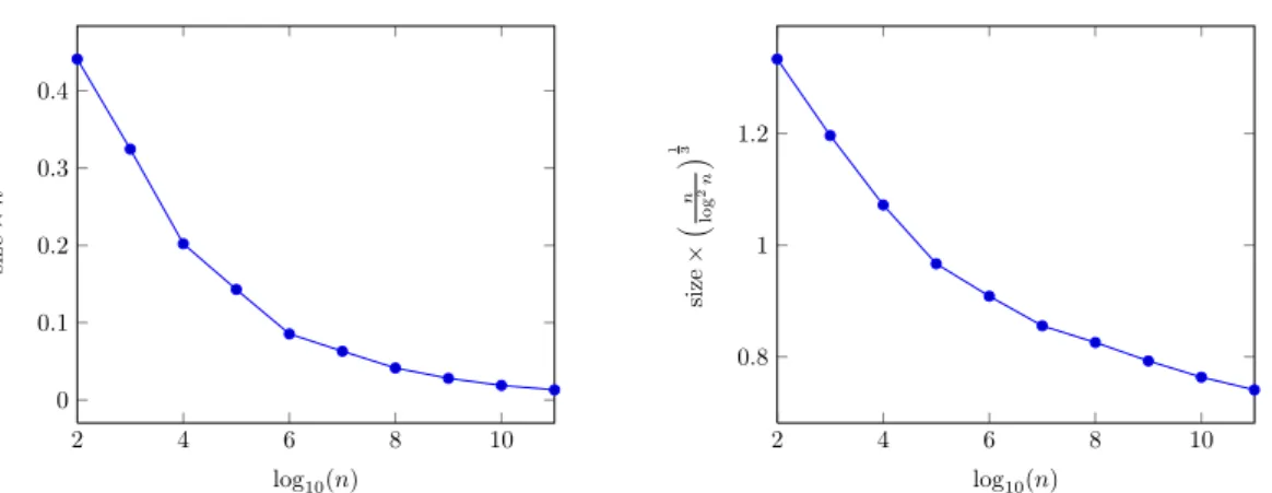
As a first application, we can estimate the distribution of the smallest and the largest edge of a random polytope, see Figure 5 and Figure 6. The average have been done on 100 experiments
for each value of log10n. The expected minimal edge seems to be O(n
−1
3), and the maximal
OÄlogn2nä
1 3 .
8 O. Devillers, P. Duchon & R. Thomasse 2 4 6 8 10 0 0.1 0.2 0.3 0.4 log10(n) si ze × n 1 3
Figure 5: Average length of the minimal edge
2 4 6 8 10 0.8 1 1.2 log10(n) si ze × Ä n lo g 2n ä 1 3
Figure 6: Average length of the maximal edge
5
Conclusion
We propose an algorithm that generates random polygons given by the convex hull of random points, without generating all the points. There is no theoretical obstacle to generalize to higher dimension. The theoretical results used for the evaluation of the complexity are known in arbi-trary dimension [Bár89, Rei10], so the analysis can be done as well.
We can reduce the expected time complexity by a logarithmic factor if we allow to increase the expected size complexity by a logarithmic factor. Instead of bounding the simulated points at
step i by n
log2n when mi becomes bigger than logn2n, we can choose to always simulate mi points.
In this case, Eki= O(m 1 3 i log 2 3m i) = O(n 1 3log 2 3n) (7)
so the expected size complexity becomes O(n13log
2
3n). On the other hand, the expected time
complexity is reduced to O(n13log
2 3n), as Ek =X i Eki = O Ñ log23n Ñ logX2n i=1 m 1 3 i éé = OÄn13log 2 3n ä . Acknowledgments
This work was initiated during the 2013 Presage Workshop on computational geometry and probability in Valberg. The authors wish to thank all the participants for creating a pleasant and stimulating atmosphere and Pierre Calka for discussions about potential use of the generator.
References
[AS08] Noga Alon and Joel H. Spencer. The probabilistic method. Wiley-Interscience Series
in Discrete Mathematics and Optimization. John Wiley & Sons Inc., Hoboken, NJ, third edition, 2008. With an appendix on the life and work of Paul Erdős.
A generator of random convex polygons in a disc 9
[Bár89] Imre Bárány. Intrinsic volumes and f -vectors of random polytopes. Mathematische
Annalen, 285(4):671–699, 1989.
[Bá92] Imre Bárány. Random polytopes in smooth convex bodies. Mathematika, 39:81–92, 6
1992.
[CSRL01] Thomas H. Cormen, Clifford Stein, Ronald L. Rivest, and Charles E. Leiserson. In-troduction to Algorithms. McGraw-Hill Higher Education, 2nd edition, 2001.
[Gra72] Ronald L. Graham. An efficient algorith for determining the convex hull of a finite
planar set. Information processing letters, 1(4):132–133, 1972.
[Rei10] Matthias Reitzner. Random polytopes. In New perspectives in stochastic geometry,
pages 45–76. Oxford Univ. Press, Oxford, 2010.
RESEARCH CENTRE
SOPHIA ANTIPOLIS – MÉDITERRANÉE
2004 route des Lucioles - BP 93 06902 Sophia Antipolis Cedex
Publisher Inria
Domaine de Voluceau - Rocquencourt BP 105 - 78153 Le Chesnay Cedex inria.fr