HAL Id: hal-02987566
https://hal.inria.fr/hal-02987566v2
Submitted on 7 Nov 2020HAL is a multi-disciplinary open access
archive for the deposit and dissemination of sci-entific research documents, whether they are pub-lished or not. The documents may come from teaching and research institutions in France or abroad, or from public or private research centers.
L’archive ouverte pluridisciplinaire HAL, est destinée au dépôt et à la diffusion de documents scientifiques de niveau recherche, publiés ou non, émanant des établissements d’enseignement et de recherche français ou étrangers, des laboratoires publics ou privés.
Taming Disruptive Base Pairs to Reconcile Positive and
Negative Structural Design of RNA
Hua-Ting Yao, Jérôme Waldispühl, Yann Ponty, Sebastian Will
To cite this version:
Hua-Ting Yao, Jérôme Waldispühl, Yann Ponty, Sebastian Will. Taming Disruptive Base Pairs to Reconcile Positive and Negative Structural Design of RNA. RECOMB 2021 - 25th international con-ference on research in computational molecular biology, Apr 2021, Padova, France. �hal-02987566v2�
Taming Disruptive Base Pairs to Reconcile Positive and Negative
Structural Design of RNA
Hua-Ting Yao1,2 J´erˆome Waldisp¨uhl2 Yann Ponty1∗
Sebastian Will1†
1LIX, CNRS UMR 7161, Ecole Polytechnique, Institut Polytechique de Paris, France 2School of Computer Science, McGill University, Montreal, H3A 0E9, Canada
Abstract
The negative structural design of RNAs, also called Inverse folding, consists in building a synthetic nucleotides sequence adopting a targeted secondary structure as its Minimum Free Energy (MFE) structure. Computationally an NP hard problem, it is mostly addressed as an op-timization task and solved using (meta-)heuristics. Existing methods are frequently challenged by demanding instances, and typically produce a single design, hindering practical applications of design, where multiple candidates are desirable to circumvent the idealized nature of design models.
In this work, we introduce RNA POsitive and Negative Design (RNAPOND), a sampling
ap-proach which generates design candidates exactly from a well-defined distribution influenced by positive design objectives, including affinity towards the target and GC-content. Negative design principles are captured by an original iterative approach, where a subset of Disruptive Base Pairs (DPBs) are identified at each step, and subsequently forbidden from pairing by the introduction of suitable constraints.
Despite the NP-hardness of the associated decision problem, we propose a combinatorial sam-pling algorithm which is Fixed Parameter Tractable (FPT) for the tree-width of the constraint network. Our algorithm, coupled with a suitable rejection step and an automated inference of DPBs, achieves a similar or better level of success in comparison to the state of the art, while allowing for the generation of diverse, thermodynamically efficient, designs. Interestingly, it also automatically recovers some of the strategies used by practitioners of RNA design.
RNAPONDis an open source project, available at:
https://gitlab.inria.fr/amibio/RNAPOND
∗
Co-corresponding Author. Email: yann.ponty@lix.polytechnique.fr †
1
Introduction
Rational RNA design encompasses a wide range of computational methods aiming at the generation of RNA sequences performing certain biological functions. At the core of design efforts, one finds the negative design problem, also called inverse folding in the literature, which targets the production of a nucleotide sequence that adopts a given target structure as its Minimum Free-Energy (MFE) structure. Thus, any solution for negative design must achieve greater affinity towards its target than any of its alternative structure. Due to its NP-hardness, popular methods for the negative RNA design mostly rely on meta-heuristics, stochastic optimization and constraint programming, with a recent burst of interest in Machine Learning [1, 2, 3].
By contrast, positive RNA design attempts to optimize, or simply bias, affinity towards a given target. Computationally, positive design tasks can typically be solved exactly in polynomial time [4], using approaches that capture complex energy models and a prescribed GC content [5]. Additional constraints can be accommodated, including multiple target structures [6, 7, 8], for-bidden/forced sequence motifs [9], dinucleotide content or encoded amino-acid sequence [10]. Yet, despite its flexibility, positive design cannot rule out the existence of alternative stable structures, often preventing the produced sequences to preferentially adopt its target at the thermodynamic equilibrium. Indeed, there is currently no method that simultaneously and efficiently offers the fine level of control enabled by positive design, and the structural specificity of negative design, while both are typically required in the context of synthetic biology [11, 12].
Our method, called RNAPOND(RNA POsitive and Negative Design), attempts to reconcile posi-tive and negaposi-tive design, and stems from the following observation: Upon MFE folding, posiposi-tively- positively-designed RNAs usually differ from their target structure due to the formation of very specific Disruptive Base Pairs (DBPs), that both recurrently represented and reproducible across random data sets. Examples of such base pairs include helix extensions in both basal and apical regions, or within interior loops, usually associated with a negative selective pressure within RNA multi-ple sequence alignments [13], and are the object of explicit countermeasures from practitioners of RNA design [14, 8]. This suggests a simple automated strategy, that iteratively samples design candidates using positive design principles, identifies a set of dominant DPBs and forbids them for future iterations, unless they induce some inconsistency.
Implementing such a strategy requires the capacity to randomly generate RNAs that simul-taneously support those base pairs in the target, being assigned canonical G-C, A-U and G-U contents, while forbidding the pairing of positions involved in DBPs (assigned to them unpairable nucleotides). Prior to adding a DBPs, one must test that its addition does not break the consistency of constraints, i.e. that there exists a sequence that satisfies all constraints. Despite the existence of a polynomial-time algorithm for a similar problem [15], this problem turns out to be NP hard even when restricted to a single, pseudoknot-free, secondary structure. Nevertheless, we obtain a Fixed-Parameter Tractable algorithm for the tree-width, based on dynamic programming compu-tation of a dual partition function, which extends into an exact sampling algorithm for admissible sequences within a Boltzmann-Gibbs distribution. RNAPONDis very efficient in practice and, despite the simplicity of its iterative strategy, reveals competitive with the current state-of-the-art.
We present in Sec. 2 some necessary definitions, and a precise statement of our core compu-tational problems. We establish complexity results and provide FPT exact decision and sampling algorithms in Sec. 3. In Sec. 4, we describe their integration within RNAPOND, and its implemen-tation details. In Sec. 5, we perform an empirical assessment of RNAPOND in comparison with the current state of the art, and conclude in Sec. 6 with future considerations and extensions.
A C G U A C G U A U C A U G C C G C A A
1
2
3
4
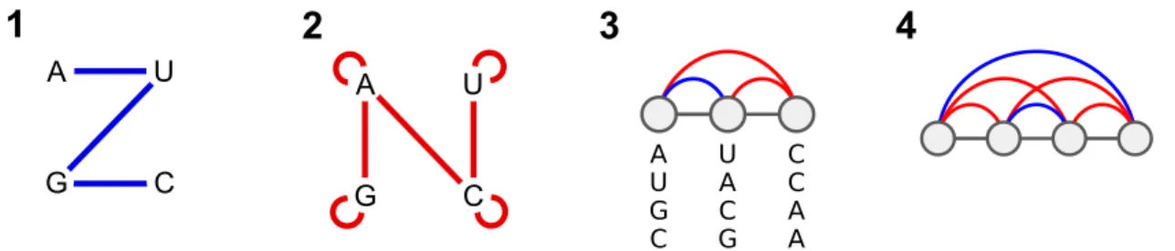
Figure 1: Graph representations for set B of compatible nucleotides pairs (1), and set B of incom-patible nucleotides (2). (3) Example of consistent secondary structure S = {(1, 2)} and disruptive base pairs D = {(1, 3), (2, 3)}, inducing a partition function value of 4 for β = 0, i.e. only 4 out of the 64 possible nucleotide assignments satisfy the constraints induced by S and D. (4) Minimal example of inconsistent instance, i.e. any RNA sequence violates at least one of the constraints.
2
Definitions and problem statements
An RNA can be abstracted as a sequence w over the alphabet Σ := {A, C, G, U} of length n = |w|. Through hydrogen bonding, the positions of an RNA w can form base pairs (i, j) ∈ [1, n]2, i < j,
such that (wi, wj) ∈ B, with B := {(C, G), (G, C), (A, U), (U, A), (G, U), (U, G)} representing the set
of valid pairs of nucleotides. In the following, we denote by B := Σ2\ B the pairs of nucleotides that are unable to form canonical interactions.
A secondary structure for an RNA w is a set S ⊂ [1, n]2 of base pairs, such that: i) Any given position cannot be involved in more than one base pair in S; ii) Any pair (i, j) ∈ S must observe a minimal distance θ, i.e. j − i > θ; iii) Any pair (i, j) ∈ S must be valid for w, i.e. (wi, wj) ∈ B;
iv) Pairs in S are pairwise non-crossing, i.e. @(i, j), (k, l) ∈ S such that i < k < l < j. Throughout the rest of the document, we will denote by Sw the set of secondary structures that are compatible
with an RNA w.
Given a secondary structure S ∈ Sw, we denote by Ew(S) ∈ R the real-valued free-energy of S
in the context of w. We can then formally define the negative design problem.
negative-design problem
Input: Secondary structure S, length n
Output: RNA sequence w, |w| = n, such that, ∀S06= S ∈ Sw, Ew(S0) > Ew(S)
This problem is NP-hard even in simple energy models [16], and currently does not admit an exact parameterized algorithm.
In this work, we identify and forbid disruptive base pairs (DBPs) by forcing their assignement to unpairable nucleotides in B. DBPs are base pairs that are recurrent within the stable alternative folds of design candidates generated from positive design principles. Preventing such DPBs from forming is key to satisfying both positive and negative design constraints.
A key component of our approach is therefore an algorithm for sampling admissible sequences, defined as compatible with a target input structure, but also incompatible with a predefined set D of DBPs. Let us denote by WS,D,n := {w0 ∈ Σn | w ∈ Sw0 and ∀(w0
i, w0j) ∈ B, (i, j) ∈ D} the set
of admissible sequences for S and D. In the spirit of the recursive method in enumerative combi-natorics [17], successfully adapted to RNA structure prediction [18] and design [5], our approach starts with a preprocessing step, the computation of an (extended dual) partition function over WS,D,n, followed by a stochastic backtrack.
extended-partition-function problem
Input: Sec. struct. S, length n, set D ⊂ [1, n]2 of disruptive BPs, constant β ∈ R+ Output: Extended (dual) partition function Z(S, D, n) ∈ R+ such that
Z(S, D, n) = X
w0∈W S,D,n
e−β.Ew0(S)
Finally, we denote by consistency the decision version of this problem which asks whether or not the constraints induced by S and D can be jointly satisfied or, equivalently, if an admissible sequence exists (|WS,D,n| > 0 ⇒ True, WS,D,n = ∅ ⇒ False). This property is used to decide if a
DBP can be safely added, and solving the problem is an important part of our method.
3
Computational results
In the absence of DBPs (D = ∅), the compatibility constraints induced by a target structure can always be satisfied [4] since the graph of the combined structures is bipartite. If the target is the open chain (S = ∅), constrained to avoid a set D of DBPs, then any mononucleotidic sequence will satisfy D, so the problem is again trivially solved by returning True. Combining those two types of constraints constitutes an open problem, and turns out to induce substantial difficulties.
3.1 Complexity results
The decision version consistency of extended-partition-function is closely related to the polynomial-time solvable realizability of extended shapes, considered by Hellmuth et al [15]. realizability takes as input multiple target secondary structures, and pseudo base pairs whose associated positions are prevented from pairing in the output sequences by being assigned nu-cleotides in {(A, A), (C, C), (G, G), (U, U)}. Consequently, there is a solution for realizability if and only if the combined structure graph is bipartite after identifying all nodes connected by the pseudo base pairs [4]. Surprisingly, this minor difference turns out to be sufficient to greatly increase the computational hardness of the problem.
Theorem 1. consistency is NP-hard
Proof. The NP-hardness is shown by a polynomial-time reduction from 3-sat to consistency. Namely we show that an efficient algorithm for consistency would imply that 3-sat can be solved efficiently, a fact that is highly unlikely as it would imply that P = NP.
3-sat problem
Input: Boolean formula Φ over variables x1, . . . , xn in 3-Conjunctive Normal Form
Output: True if a satisfying assignment exists, False otherwise.
Notice that, as shown in Fig. 1, any instance (S, D) of consistency can be represented as a graph over positions in [1, n], with edges induced by the target (blue) and disruptive base pairs (red). For a graph or subgraph, an admissible sequence corresponds to an assignment µ : VΦ → Σ
of nucleotides to the vertices VΦ, which satisfies the constraints induced by the edges. For any
(a) (b) v4 w4 v6 w6 v7 w7 v1 ` w1 v5 w5 w3 v3 w2 v2 x1 x3 x3 x2 x6 x7 x6 x5 (c)
Figure 2: (a) Gadget G for the boolean clause (x1∨ ¯x2∨ x3). Vertices representing literals of the
clause are drawn in green. (b) Design converted from a satisfying assignment of (l1∨ l2∨ l3), where
l1 (u1) is assumed to be True (C). u2 and u3 are either C or G based on its value l2 and l3 in the
assignment. (c) Gadget of formula (x1∨ x2∨ x3) ∧ (x2∨ x4∨ ¯x5) ∧ ( ¯x3∨ x6∨ ¯x7).
• For each variable xi occurring in Φ, GΦ contains two special variables vertices vi and wi,
connected with a blue base pair (from S);
• Each clause ck in Φ translates within GΦ into a gadget Gk, as shown in Fig. 2a. Gk is a
subgraph of an instance graph, where 3 vertices (u1, u2, u3) are distinguished to represent the
3 literals in ck = (l1∨ l2∨ l3), each identified with a suitable variable vertex (ui = vi if li = xi,
and ui = wi for li = ¯xi)
Fig. 2c shows the graph GΦobtained for the formula Φ = (x1∨x2∨x3)∧(x2∨x4∨ ¯x5)∧( ¯x3∨x6∨ ¯x7).
Lemma 1. Let Gk be one of the gadgets, involving variable vertices (u1, u2, u3). Then an admissible
assignment µ exists for Gk if and only if at least one of (µ(u1), µ(u2), µ(u3)) is in {A, C}.
Sketch of proof. It can be verified by case decomposition that assigning (u1, u2, u3) to {G, U} leads
to a contradiction. Moreover, an inspection of Fig. 2b shows that assigning A (resp. C) to one of the variable vertices allows the two others to take value G/A/C while maintaining admissibility.
It can be shown that (u1, u2, u3) can be further restricted to C and G: if there exists an admissible
assigment µ for a given triplet (µ(u1), µ(u2), µ(u3)), then there also exists µ0that is both admissible,
and features the triplet obtained by substituting A → C and U → G.
Turning to GΦ, note that any admissible µ induces an admissible assignment for each Gk. It must
also feature coherent values on variable nodes, so that µ(vi) ∈ {A, C} implies that µ(wi) ∈ {G, U}
and vice versa. Interpreting µ(vi) ∈ {A, C} as xi = True (and {G, U} as False) we get an assignment
that satisfies each clause (Lemma 1), and thus satisfies Φ.
Conversely, from a Boolean assignement (x1, . . . , xn) that satisfies Φ, we obtain an assignment
µ for GΦ by setting (µ(vi), µ(wi)) := (C, G) (resp. (G,C)) if xi = False (resp. True). For each
gadget Gk, at least one of the variable vertices is True → C, otherwise ck would be falsified, and an
admissible assignment can be found for the other positions as per Fig. 2b. Finally, each vertex in GΦ is connected with at most one blue edge, so there exists an instance (SΦ, DΦ) that induces GΦ
(ordering vertices so that blue base pairs in SΦ do not cross).
We conclude that a solution exists for Φ if and only if there is an admissible sequence for (SΦ, DΦ), so that solving consistency provides an answer to 3sat. Since (SΦ, DΦ) has size linear
Algorithm 1: Tree decomposition-based dynamic programming algorithm for extended partition function.
1 Function ExtendedPartitionFunction(S, D, n, β):
2 T = (V, E) ← Tree decomposition of G = ([1, n], S ∪ D);
3 Assign each (i, j) ∈ S ∪ D to exactly one node of T that contains both i and j; 4 foreach node u ∈ V in post-order do
5 foreach nuc. assignment a := (a1, . . . , ax) to pos. shared by u and its parent in T do 6 Initialize partition function of node to Zu[a] ← 0;
7 foreach nuc. assignment b := (b1, . . . , by) to positions in u and not its parent do 8 if a ∪ b compatible with base-pair(s) and DBPs assigned to u then
9 Increment node part. fun. to include contribution of assignment a ∪ b:
Zu[a] += Y
(i,j)∈S assigned to u
e−β·E(i,j) Y
v child of u
Zu[cv]
where cv denotes the restriction of a ∪ b to positions shared by u and v;
10 return The extended partition function Zroot(T )[∅]
on the number of clauses in Φ, this implies the hardness of consistency.
Moreover, setting β = 0 leads to Z(S, D, n) = |WS,D,n|, so solving
extended-partition-function provides an immediate answer to consistency. Corolary 1. extended-partition-function is NP-hard
Now, given an instance (S, D, n) we define its associated compatibility graph G as:
G = ([1, n], S ∪ D). (1)
As will be shown in the Subsection 3.2, the problem can be solved in time polynomial in |S| and |D| as long as t, the tree-width of G, is bounded by some constant.
Proposition 1. extended-partition-function is FPT for the tree width of G.
Again, consistency can be determined from the value of the extended setting at β = 0. Corolary 2. consistency is FPT for the tree width of G
3.2 Fixed Parameter Tractable (FPT) algorithms
Our approach to solving extended-partition-function exactly is inspired by the Cluster Tree Elimination framework [19], which perform efficient belief propagation in graphical models. It builds on our algorithm RNARedPrint [8], and is easily generalizable to support multiple target structures, more sophisticated energy models and constraints.
Theorem 2. Algorithm 1 solves consistency and extended-partition-function in time Θ((n+ |D|) · 4w) and space Θ(n · 4w) where w is the tree width of G = ([1, n], S ∪ D).
Algorithm details and proof sketch. Dynamic programming is enabled by a the tree decomposition T = (V, E) for G: 1. each position i ∈ [1, n] occurs in some v ∈ V , 2. the positions of each edge (i, j) of G simultaneously occur in some node v ∈ V , 3. for each i ∈ [1, n], the induced subgraph of T consisting of the nodes v ∈ V, i ∈ v is connected. Furthermore, children in T shall contain at most one variable that does not already occur in the parent. Despite being a NP-hard problem for general graphs, a tree decomposition minimizing the tree width can be computed in polynomial time for graphs of bounded tree width.
The DP algorithm tabulates, at each of the Θ(n) nodes, the partition functions for all nucleotide combinations of the shared position with its parent. Thus, the largest table consists of 4w partition functions, which explains the space complexity. For each node, the computation iterates over the nucleotide combinations of at most w + 1 positions; this bounds the time complexity. Finally, the total partition function can be found at the root node.
Example. In Fig. 3 at node {2, 5, 6}, the algorithm computes the two-dimensional table Z{2,5,6}
(to be available in the computation at its parent node {2, 6}). Assume that the constraint due to DBPs (2, 5) and the base pair (2, 6) have been been assigned to node {2, 5, 6}. Thus, the algorithm calculates all partition function for nucleotides x,y,z at respective positions 2,5,6. It considers only combinations, where (x, y) 6∈ B, other combinations have partition function 0. For table entry Z{2,5,6}[x, z], it marginalizes (i.e., sums) over all y, where the partial partition function for x, y, z is
Z{1,6}[x] · Z{3,5,6}[y, z] · exp(−β.E(y, z)), where Z{1,6}and Z{3,5,6} denote the tables of the children.
Finally, Algorithm 1 can be adapted into a stochastic backtrack procedure, as shown in Ham-mer et al [8]. We obtain an exact sampling algorithm for the Boltzmann-Gibbs distribution over RNA sequences, such that any sequence in WS,D,n is emitted with probability
P(w | S, D) = e
−β.Ew0(S)
Z(S, D, n). (2)
This sampling algorithm generates k sequences in linear time Θ(k·(n+|D|)), after a precomputation of the dual partition function in time Θ(4w· (n + |D|)).
4
The
RNAPOND
method for RNA inverse folding
Our method, named RNA Positive and Negative Design (RNAPOND), is inspired by the manual refinement by humans when tackling the task in practice. Its foundation is inspired by the obser-vation that some base pairs and structural motifs, e.g. competing helices, more likely than others interfere with the folding of sequences generated from positive design principles. The key idea of our method is to iteratively identify such recurrent Disruptive Base Pairs (DBPs) and prevent them from occurring in the MFEs of subsequent rounds by adding suitable constraints.
1 2 3 4 5 6 2,5,6 1,6 3,5,6 5 2 6 1 4 3 {} {2} 2,6 {} 4 2 {6} {26} {56}
Figure 3: Small compatibility graph and its tree decomposi-tion. Left – Compatibility graph of an RNA of length 6, with edges induced by target base pairs (blue) and DBPs (red). Right – Valid tree decomposition of the graph, with each node labeled by its assigned sequence positions (node in compatibil-ity graph), and each edge labeled with positions of the child nodes that are shared (purple) or not (green) with its parent.
1 10 20 30
1 10 20 30
1 10 20 30
Sampling DBPs
Inference
Disruptive Base Pairs (DBPs)
Main loop Final DBP set Extended sampling 1 10 20 30 1 10 20 30 Target structure S Input Admissible sequences Designs Output Boltzmann base pairin g pr obability Ensemble analysis Yes No CGCCCUUAAUGGAUGCA... GGGCGAUUUACGAAGCU... GGUCCUUACCGGAACGA... CGCCCUCAUUGGAGCAC... CCCCGAUAUACGAUGCG... UCGCCAUUAGGGUUGCU... Initialization Evaluation ∃w s.t. MFE(w)=S?
Target base pairs
Expected base pairing profile Consistent updated DPBs
Figure 4: General strategy of RNAPOND for the inverse folding of RNA. From an input target structure, an initial set of likely-disruptive base pairs (DPBs) is inferred. At each iteration, new candidate DBPs are inferred by a joint thermodynamic analysis and, if consistent with existing constraints, are added to the list of DPBs. Once some solutions are found, a deeper sampling produces independent and diverse designs for the target.
As illustrated in Fig. 4,RNAPONDtakes as input a secondary structure S in dot-bracket notation and, considering a set D of DBPs that is initialized to helix extensions, iterates the following steps: 1. Sampling: Generate k RNA sequences w := w1, . . . , wk, from the Boltzmann distribution
over sequences that are compatible with the secondary structure (S) and DPBs (D);
2. Inference of DBPs: Identify and add to D the d most disruptive base pairs, having highest expected Boltzmann probability within the sample w), such that: a) (i, j) is not in the target structure S; and b) constraints induced by S and D ∪ {(i, j)} remain consistent (see Sec. 2); 3. Evaluation of candidates: Compute the MFE structure Si?of each sequence wi, and report
its base-pair distance to S.
These steps are repeated until a solution is found, or the tree width of the graph induced by S and D exceeds a predefined threshold. Finally, if a solution is found, the method executes a final round of upsampling/evaluation using K k, to allow the generation of several (diverse) solutions.
RNAPONDis implemented in Python3+ based on the C++/Python framework infrared [20]; moreover,
it relies on the ViennaRNA 2.4.x library [21] and NetworkX for the tree decomposition.
Initialization. To spare RNAPOND from inferring trivial DBPs, we initialize D to prevent helix extensions. We set D to include base pairs, extending the basal and apical regions of each helix. Sampling. We use a simplified energy model, additive on base pairs yet aware of stackings, as done in Hammer et al [8], which was shown to achieve an almost perfect correlation (R = 0.95) with the Turner energy. We implemented the sampling – including the partition function computation by Algorithm 1 – using the infrared framework [20]. infrared enables controlling the GC-content as in Reinharz et al [5]; here, we further distinguish between paired and unpaired target regions. Inference of disruptive base pairs (DBPs). DPBs are identified based on an expected base pairing profile, obtained by averaging the probability matrices produced by the ViennaRNA [21] implementation of the McCaskill algorithm [22]. Base pairs that are not in S are then considered
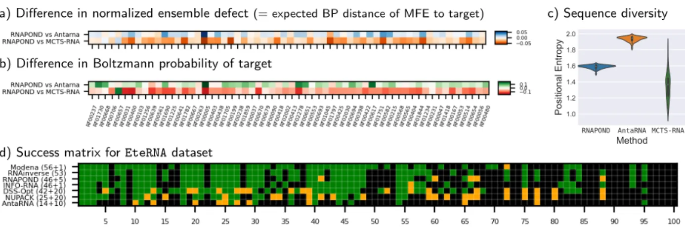
a) Difference in normalized ensemble defect(= expected BP distance of MFE to target)
b) Difference in Boltzmann probability of target
c) Sequence diversity
RNAPOND AntaRNA MCTS-RNA
d) Success matrix for EteRNA dataset
Figure 5: Results ofRNAPONDand competitors on AntaRNA/RFAM targets and EteRNA puzzles. Anal-ysis of (a) ensemble distance, (b) equilibrium probability and (c) sequence diversity of solutions produced for the AntaRNA/RFAM dataset. (d) Success matrix ofRNAPONDand competitors on EteRNA dataset. Green squares indicate success, i.e. at least one solution for the given target/puzzle. Or-ange squares indicate near success (MFE within 2 BPs of target).
in decreasing order of probability. One then checks adding it to D will retain consistency, using the partition function of the extended instance as described in Sec. 3.
Parameter values. We sample by default k = 200 sequences per iteration, in order to achieve a tradeoff between the stability of the inference step, and the computational overhead of running the McCaskill algorithm for each sequence.
5
Validation and comparison to state of the art
Datasets. We focused our validation effort on two recent collections of target structures.
The AntaRNA/RFAM dataset [23] consists of a selection of targets extrapolated from RFAM [13] consensuses. For each of the selected family, the consensus structure was mapped onto the smallest sequence of the family, avoiding the artificial insertion of long unpaired regions. We further removed isolated base pairs from those 63 realistic structures, having length range from 36 to 274 nts and showing a typical proportion of paired positions (35% to 80%, median=53%).
The EteRNA dataset [14] is a collection of 100 artificial puzzles, designed to challenge participants of a crowdsourced initiative/gaming. While arguably pathological and not representative of typical design tasks – with certain targets featuring long unpaired regions, very limited structure or even an overwhelming proportion of isolated pairs and stackings – those challenging targets are nevertheless informative as a stress test for our approach, as will be further shown.
Benchmark execution. We consideredRNAPONDand selected competitors, including AntaRNA [23], MCTS-RNA [24], MODENA [25], RNAinverse [26], INFO-RNA [27], NUPACK [28] and DSS-OPT [29], invoked as described in App. B. Candidate sequences were then validated by computing their MFE structure with the ViennaRNA package 2.4.14, and reporting their base-pair distance to the target.
For the AntaRNA/RFAM dataset, we used the Turner 2004 nearest neighbor model for the tool configuration and verification of candidates. We comparedRNAPONDto the state of the art AntaRNA and MCTS-RNA, which both support Turner 2004.
• EteRNA puzzle 37 – “Water Strider”
0 5 10 15
Base pair distance 101
102
Frequency init+15
init+6 init a. Distribution of BP dist. to target
w/o init init+3 init+6 init+9 init+15
0 50 100 150
b. #Solutions per iteration c. Final set of disruptive base pairs
• EteRNA puzzle 58 – “Multiloop...”
d. Final set of DBPs for EteRNA 58
• EteRNA puzzle 22 – “This is ACTUALLY Small And Easy”
1 10 20 30 40 50 60 70 80 90 100 110 120 130 140 150 160 170 180 190 200 210 220 230 240 250 260 270 280 290 300 310 320 330 340 350 360 370 380 390 400
e. Final set of DBPs for EteRNA 22
Figure 6: Illustrating the behavior ofRNAPOND on three exemplary EteRNA targets (37, 58 and 22). For EteRNA 37: (a) Impact of added DPs on the distribution of distances to target within 50· 103 sampled sequences; (b) Number of solutions per iteration; (c) Target structure and final set of DBPs. Secondary structures and final DBPs for EteRNA 58 (d) and EteRNA 22 (e).
Since the EteRNA game and dataset were designed explicitly for the Turner 1999 model, we used this model for optimization and validation. Some approaches, such as MCTS-RNA and a recent reinforcement learning approach [30], do not currently support Turner 1999. Thus we left out of the benchmark, but report the performance of the former in App. B. Each software was executed with a time limit of 5 min per instance on a notebook with i7-7500U CPU.
Analysis of AntaRNA/RFAM results. In term of success, we observe excellent performances for both
RNAPOND, AntaRNA and MCTS-RNA. All methods solve all targets, except RF01241, RF00906 and
RF00446. For those 3 instances, the best MFE distances to the target are of 1, 1 and 2 respectively for all three tools, suggesting that a solution may simply not exist. Despite the stochastic aspects
of RNAPOND, we observed a good level of robustness of our method, with three independent runs
showing successful on the exact same instances, and achieving same distance to target otherwise. A closer look reveals further differences in performance with respect to negative design met-rics, including Ensemble Defect [28] (Fig. 5a) and the Boltzmann probability [22] of the target structure (Fig. 5b). Interestingly, RNAPOND shows an average normalized ensemble defect of 0.076 and Boltzmann probability of 22.2%), and dominates AntaRNA (0.085/17.8%) with respect to those two metrics, demonstrating its capacity to embrace negative design principles, although MCTS-RNA (0.056/28.7%) remains superior to both. This trend is inverted when considering the diversity of sequences generated by each tool, as measured by the Positional (Shannon) Entropy, reported in Fig. 5c. HereRNAPOND(avg 1.6 bits/nt), in its current state, does not match the excellent diversity of AntaRNA (1.95 bits/nt), but greatly exceeds that of MCTS-RNA (1.38 bits/nt).
Analysis of EteRNA results. On the challenging EteRNA dataset, RNAPOND solves 47 of the 100 instances exactly (MFE structure matching the target). For 7 further instances, we find near-solutions that are close to the target (MFE within 2 BPs of target). For comparison, we report in Fig. 5 the success, and near-success if available, of several competitors.
Case study A – EteRNA 37. We considered this, relatively easy, puzzle to investigate the effect of DBPs on the distribution of distance to the the target. Using RNAPOND, we generated 50· 103 samples for the sets of DBPs introduced by the first 5 iterations of RNAPOND, consider no DBP as a control. As shown in Fig. 6a, the introduction of DBPs successfully shifts the probability distribution towards solutions, and the probability of sampling a solution appears to increase exponentially (Fig. 6b), from 0/50· 103 in the absence of DPBs to 155 after 5 rounds (init+15 DBPs) . The final set of constraints (DBPS of Fig. 6c) is sparse, and appears to essentially delimit helices, forbidding their bi-directional extension. Interestingly, this strategy typical of manual design practitioners, and is recovered byRNAPONDdespite not being one of its design choice. Case study B – EteRNA 58. On this example,RNAPONDfinds his first solution after generating 9 initial DBPs, supplemented by 30 more DBPs introduced over 10 rounds (Fig. 6). Remarkably, DBPs are not only introduced to avoid helix extensions, but also unwanted interactions within the large multi-loop. This is achieved through the introduction of key local stack-like DPBs which appear sufficient to break the symmetries presented by the multiloop.
Case study C – EteRNA 22. This challenging target (see Fig. 6e) consists of 400 unpaired nucleotides, and could not be solved within the time limit. It is easy to solve manually by only using unpairable nucleotides, but we decided to ignore such an ad hoc rule, both to ensure maximal sequence diversity and to preserve the level of generality ofRNAPOND. Interestingly, lifting the time limit, yields a solution after 4 h and 154 rounds, introducing 462 DBPs (see Fig. 6e). Those incompatibility constraints are surprisingly local, with the exception of DBPs connecting the 5’ and 3’ ends, and suggests that forbidding small hairpins may be sufficient to design large loops within challenging RNAs.
6
Discussion
In this work, we presented RNAPOND, a new method for RNA inverse folding, combining positive and negative design objectives. Powered by a Fixed-Parameter-Tractable algorithm for sequence sampling, it does not include any local optimization of individual sequences, but rather adapts its sampled distribution to favor solutions, based on an identification/avoidance of disruptive base pairs. Despite its simplicity, this strategy is already sufficient to achieve performances that are comparable or better than the state of the art. Overall, these results support the notion that
RNAPOND achieves an excellent trade-off between exploration, the optimization of negative design
criteria, and exploitation, witnessed by a sizable sequence diversity.
Contrasting with recent approaches, our method is unsupervised and driven by a simple common-sense rule. The fact that it is sufficient to solve so many instances is, in our opinion, remarkable, and speaks for the potential of future extensions. It also bears interesting consequences for RNA structural evolution. Indeed, its success in designing complex RNA architectures suggests that a local selective pressure may often be sufficient to implement negative design principles, allowing the evolution of complex RNA architectures.
Extensions of this work are numerous, and include: more sophisticated energy models, par-ticularly to support pseudoknots, non-canonical modules or multiple target structures [8]; the combination with local search heuristics for further refinements, i.e. towards a glocal approach [5]; more expressive negative constraints (unpaired regions, stacking pairs). The algorithmic framework utilized in this work is already amenable to many such extensions, in a declarative manner.
References
[1] Shi, J., EteRNA players, Das, R. & Pande, V. S. Sentrna: Improving computational RNA design by incorporating a prior of human design strategies (2018). ArXiv:1803.03146.
[2] Runge, F., Stoll, D., Falkner, S. & Hutter, F. Learning to design RNA. In Proceedings of ICLR 2019 (2019).
[3] Angenent-Mari, N. M., Garruss, A. S., Soenksen, L. R., Church, G. & Collins, J. J. A deep learning approach to programmable RNA switches. Nature communications 11, 5057 (2020).
[4] Flamm, C., Hofacker, I. L., Maurer-Stroh, S., Stadler, P. F. & Zehl, M. Design of multistable RNA molecules. RNA (New York, N.Y.) 7, 254–265 (2001).
[5] Reinharz, V., Ponty, Y. & Waldisp¨uhl, J. A weighted sampling algorithm for the design of RNA sequences with targeted secondary structure and nucleotide distribution. Bioinformatics 29, i308–i315 (2013).
[6] H¨oner Zu Siederdissen, C. et al. Computational design of RNAs with complex energy land-scapes. Biopolymers 99, 1124–1136 (2013).
[7] Hammer, S., Tschiatschek, B., Flamm, C., Hofacker, I. L. & Findeiß, S. RNAblueprint: flexible multiple target nucleic acid sequence design. Bioinformatics (Oxford, England) 33, 2850–2858 (2017).
[8] Hammer, S., Wang, W., Will, S. & Ponty, Y. Fixed-parameter tractable sampling for RNA design with multiple target structures. BMC bioinformatics 20, 209 (2019).
[9] Zhou, Y. et al. Flexible RNA design under structure and sequence constraints using formal languages. In Gao, J. (ed.) ACM Conference on Bioinformatics, Computational Biology and Biomedical Informatics. ACM-BCB 2013, 229 (ACM, 2013).
[10] Zhang, Y., Ponty, Y., Blanchette, M., Lecuyer, E. & Waldisp¨uhl, J. SPARCS: a web server to analyze (un)structured regions in coding RNA sequences. Nucleic Acids Research 41, W480–5 (2013).
[11] Rodrigo, G., Landrain, T. E., Majer, E., Dar`os, J.-A. & Jaramillo, A. Full design automation of multi-state RNA devices to program gene expression using energy-based optimization. PLoS Computational Biology 9, e1003172 (2013).
[12] Findeiß, S., Etzel, M., Will, S., M¨orl, M. & Stadler, P. F. Design of artificial riboswitches as biosensors. Sensors (Basel, Switzerland) 17, E1990 (2017).
[13] Kalvari, I. et al. Rfam 13.0: shifting to a genome-centric resource for non-coding RNA families. Nucleic acids research 46, D335–D342 (2018).
[14] Lee, J. et al. Rna design rules from a massive open laboratory. Proceedings of the National Academy of Sciences of the United States of America 111, 2122–2127 (2014).
[15] Hellmuth, M., Merkle, D. & Middendorf, M. Extended shapes for the combinatorial design of RNA sequences. Int J Comput Biol Drug Des 2, 371–84 (2009).
[16] Bonnet, ´E., Rza˙zewski, P. & Sikora, F. Designing RNA secondary structures is hard. In Raphael, B. J. (ed.) Research in Computational Molecular Biology - 22nd Annual Interna-tional Conference, RECOMB 2018, vol. 10812 of Lecture Notes in Computer Science, 248–250 (Springer, Paris, 2018).
[17] Wilf, H. S. A unified setting for sequencing, ranking, and selection algorithms for combinatorial objects. Advances in Mathematics 24, 281 – 291 (1977).
[18] Ding, Y. & Lawrence, C. E. A statistical sampling algorithm for RNA secondary structure prediction. Nucleic acids research 31, 7280–7301 (2003).
[19] Dechter, R. Reasoning with Probabilistic and Deterministic Graphical Models: Exact Algo-rithms (Morgan & Claypool, 2013).
[20] Will, S., Ponty, Y. & Yao, H.-T. Infrared (2020). URL https://gitlab.inria.fr/swill/ Infrared.
[21] Lorenz, R. et al. ViennaRNA package 2.0. Algorithms for molecular biology : AMB 6, 26 (2011).
[22] McCaskill, J. The equilibrium partition function and base pair binding probabilities for RNA secondary structure. Biopolymers 29, 1105–1119 (1990).
[23] Kleinkauf, R., Mann, M. & Backofen, R. antaRNA: ant colony-based RNA sequence design. Bioinformatics 31, 3114–3121 (2015).
[24] Yang, X., Yoshizoe, K., Taneda, A. & Tsuda, K. Rna inverse folding using monte carlo tree search. BMC bioinformatics 18, 468 (2017).
[25] Taneda, A. MODENA: a multi-objective RNA inverse folding. Adv Appl Bioinform Chem 4, 1–12 (2011).
[26] Hofacker, I. L. et al. Fast folding and comparison of RNA secondary structures. Monatshefte f¨ur Chemie/Chemical Monthly 125, 167–188 (1994).
[27] Busch, A. & Backofen, R. INFO-RNA–a fast approach to inverse RNA folding. Bioinformatics 22, 1823–31 (2006).
[28] Zadeh, J. N., Wolfe, B. R. & Pierce, N. A. Nucleic acid sequence design via efficient ensemble defect optimization. Journal of Computational Chemistry 32, 439–452 (2011).
[29] Matthies, M. C., Bienert, S. & Torda, A. E. Dynamics in sequence space for RNA secondary structure design. Journal of chemical theory and computation 8, 3663–3670 (2012).
[30] Eastman, P., Shi, J., Ramsundar, B. & Pande, V. S. Solving the RNA design problem with reinforcement learning. PLOS Computational Biology 14, 1–15 (2018).
A
Proof of Lemma 1
Lemma (Lemma 1). Let Gk be one of the gadgets, involving variable vertices (u1, u2, u3). Then
an admissible assignment µ exists for Gk if and only if at least one of (µ(u1), µ(u2), µ(u3)) is in
{A, C}.
Proof. Consider an assignment to Gk. Suppose that the vertices (u1, u2, u3) are all assigned to
{G, U}. Without loss of generality, we assume that u1 is G (by symmetry of the roles played by G and U).
First of all, the base pair (1, 2) in the same pentagon as u1 is either (C, G) or (G, C). Otherwise,
one of the bases 1 or 6 must be U; since each nucleotide can pair with G or U, there is no valid value for vertex 8 or 7, and thus no admissible assignment. Next, the outer ring composed by six disruptive base pairs implies that vertices u2 and u3 are also G. Therefore, the three base
pairs (1, 2), (3, 4), and (5, 6) in the center hexagon are all either (C, G) or (G, C). Without loss of generality, we assume that (1, 2) is (C, G), then (3, 4) and (5, 6) are both (G, C), due to the disruptive base pairs (2, 3) and (1, 6). This yields a contradiction, since the base pair (4, 5) is disruptive, but the nucleotides assigned to 4 and 5 are C and G which can form a base pair. Thus, at least one of the variable vertices must be in {C, A}.
To conclude, we need to show that assigning one of the variable vertex to {A, C} is sufficient to ensure the existence of an admissible assignment. Fig. 2b shows that assigning A (resp. C) to one of the variable vertices allows the two others to take value G/A/C while maintaining admissibility.
B
Detailed benchmarking methodology and additional results
B.1 Tools configuration and optionsFor the EteRNA 100 benchmark, we downloaded and installed the following tools on a 64-bit GNU/Linux:
• AntaRNA from http://www.bioinf.uni-freiburg.de/Software/antaRNA/, in the version used within its main manuscript [23] (v109)
• DSS-Opt from https://github.com/marcom/dss-opt, commit c0c1e0f
• INFO-RNA from http://www.bioinf.uni-freiburg.de/Software/, version INFO-RNA-2.1.2
• RNAinverse as part of the Vienna Package 2.4.14 from https://www.tbi.univie.ac.at/RNA
• Modena from http://rna.eit.hirosaki-u.ac.jp/modena/ in version 0040
• NUPACK v3.3.2 from http://www.nupack.org, installed from source upon registration
All tools accept the target structure TARGET in the form of a dot-bracket string (also known as Vienna format). To make the results from the different tools comparable, we applied a uniform time-limit of 5 min per job (timeout 5m), but also carefully set relevant command line arguments (e.g. $iterations) for each individual tool whenever available.
We selected the Turner 1999 energy model: the tools AntaRNA, RNAinverse, INFO-RNA and NUPACK allow to provide the corresponding parameter file rna turner1999 from the Vienna package,
or provide an explicit option (NUPACK); Others come with compiled-in Turner 1999 parameters (INFO-RNA, DSS-Opt).
In Table 1, we show the concrete commands executed for each tool in the benchmark on EteRNA 100. In particular, we made the following individual choices:
• AntaRNA was executed asking for a single solution for the target structure at the default GC-content.
• RNAinverse was run in a specific mode, where it only returns one solution, when the objective of base pair distance 0 between MFE and target is met perfectly. The target structure is read from the standard input.
• For INFO-RNA, we chose settings analogous to RNAinverse. However, due to an additional termination criterion, it sometimes returns sub-optimal solutions.
• MODENA uses RNAfold in the search path, but does not allow to parametrize it; to utilize Turner 1999 parameters, we run it in combination with Vienna RNA package 1.8.5. Since MODENA returns a set of pareto-optimized solutions, we chose a best one (according to MFE–target distance) as its single solution for the purpose of this benchmark.
• All other tools were run with their default settings.
Tool Command
AntaRNA python2 antaRNA.py --Cstr TARGET -n 1 -P rna turner1999.par RNAinverse echo TARGET | RNAinverse -R-1 -P rna turner1999.par
INFO-RNA echo TARGET | INFO-RNA-2.1.2 -R -1
Modena echo TARGET >target.in ; modena -f target.in DSS-Opt opt-md TARGET
RNAPOND RNAPOND.py -n 1 --turner1999 TARGET NUPACK complexdesign -material rna1999 TARGET
Table 1: Command line calls for the EteRNA 100 benchmark
B.2 Additional AntaRNA/RFAM results
We report in Fig. 7 the successes of all 3 compared methods and, in case of failure, the min MFE distance to the target.
Figure 7: Success matrix of RNAPOND and competitors on AntaRNA/RFAM dataset. Dark squares indicate success, i.e. at least one solution for the given target/puzzle, and white squares show failure. Lighted shades of blue indicate near success (MFE within 1 or 2 BPs of target).
Figure 8: Success matrix of RNAPONDand competitors on EteRNA dataset for a 2 mins time cutoff. Green squares indicate success, i.e. at least one solution for the given target/puzzle. Orange squares indicate near success (MFE within 2 BPs of target).
B.3 Additional EteRNA results
We report results obtained using a 2 min time cutoff (Fig. 8) and additional results obtained for the standard 5 min cutoff (Fig. 9).
Interestingly, the performances of RNAPONDare very similar with times cutoffs of 2 and 5 mins. In fact, further analysis shows that most of the successes achieved usingRNAPONDare obtained after around 60 sec, while some of our competitors (e.g. INFO-RNA) seem adversely affected by such a short cutoff. Others (e.g. NUPACK) surprisingly appear to benefit from the limited allotted time, but this probably points to some level of instability. Therefore, while a more drastic cutoff would have been beneficial to the perceived performances of RNAPOND, we have preferred to consider a longer, arguably more natural, cutoff of 5 mins, both due to the timescale of experimental works following a computational design experiment, as well as out of fairness to our competitors.
Additional results reported in Fig. 9 include:
• The test of an alternative GC content of 70% for AntaRNA (AntaRNA GC 70%), reasoning that this could represent more favorable conditions for the software. Such is not the case, however, and AntaRNA solves one less problem in this setting than with 50% GC ((AntaRNA GC 70%)), as presented in the main manuscript;
• Two evaluations of the output of MCTS-RNA with respect to the Turner 1999 (MCTS-RNA 1999) and Turner 2004 (MCTS-RNA 2004) energy models. Since it was not possible to select the Turner 1999 energy model for the optimization performed by MCTS-RNA, we could not include its results in a way that would be fair to it and its competitors. Indeed, since MCTS-RNA internally uses the 2004 model, evaluating it based on the 1999 model would be unfairly detrimental to its performances (28 successes). On the other hand, evaluating it with the 2004 model would mean solving a different, potentially easier, problem than for the other tools. We therefore provide both results in this supplement for context.
Figure 9: Success matrix ofRNAPONDand extended list of competitors on EteRNA dataset for a 5 mins time cutoff. Green squares indicate success, i.e. at least one solution for the given target/puzzle. Orange squares indicate near success (MFE within 2 BPs of target).