Closed-loop market dynamics for a deregulated electric power industry

(1)

Closed-loop Market Dynamics for a Deregulated

Electric Power Industry

by

Petter L. Skantze

Submitted to the Department of Electrical Engineering and

Computer Science

in partial fulfillment of the requirements for the degree of

Master of Engineering in Electrical Engineering and Computer

Science

at the

MASSACHUSETTS INSTITUTE OF TECHNOLOGY

Febuary 1998

©

Petter L. Skantze, MCMXCVIII. All rights reserved.

The author hereby grants to MIT permission to reproduce and

distribute publicly paper and electronic copies of this thesis

rolmnf in whnlP nr

in

narL and tn

rant

others

Author...

MASSACHUSETTS INSTITUTE OF TECHNOLOGY

APR 1A2 1999

LIBRARIES

the right to do so.

Department of Electrical Engineering and

Certified by..

...

Computer Science

Febuary 4, 1998

Marija Ilic

Senior Research Scientist

. -

/

heaiSuervjsor

Accepted by...

Arthur C. Smith

Chairman, Department Committee on Graduate Students

I

(2)

Closed-loop Market Dynamics for a Deregulated Electric

Power Industry

by

Petter L. Skantze

Submitted to the Department of Electrical Engineering and Computer Science on Febuary 4, 1998, in partial fulfillment of the

requirements for the degree of

Master of Engineering in Electrical Engineering and Computer Science

Abstract

The deregulation of the electric power industry in the United States has put pressure on system operators to maintain security and performance levels under increasingly uncertain market conditions. The debate over which market structure is best suited to facilitate provision of power on a competitive basis is still ongoing. In this thesis, a summary is provided first of the effects of deregulation in the U.K. and Scandinavian markets. Based on this summary, a new market structure for trading electrical power is proposed. The trading process is separated into three markets: the long-term, spot and controls markets, distinguished by time frames as well as their functionality. Extensive modeling of the technical behavior of the system as well as the economic decision process of industry participants is introduced. A simulation of the market, driven by stochastic disturbances, shows how entirely profit-based generators adapt themselves to optimize overall social welfare. The second contribution from this thesis is the development of a new concept for market-based frequency controls. By requir-ing information about load volatility to be included in bilateral contracts, system operators will be able to provide individualized incentives for generators and loads to reduce the overall need for system control. In addition, a modification to the ex-isting criteria for frequency regulation is proposed. It is shown how by relying solely on system frequency as a control variable, an inter-area market for controls can be created. In addition to improving efficiency and taking advantage of inter-area price differentials, the new criterion also eliminates the need for real time coordination of generators participating in frequency control.

Thesis Supervisor: Marija Ilic Title: Senior Research Scientist

(3)

Acknowledgments

I would like to thank my advisor, Marija Ilic, for teaching me to trust my own ideas, and carry them through to their conclusion. Over the past two years she has become an inspiration, a mentor and a friend. Even when under the most extreme stress and pressure she has always been generous with her time and knowledge. For this I am greatly in her debt.

I would also like to thank my parents. Without their unconditional support through-out my years at MIT this thesis could never have been completed.

The discussions with Prof. Goran Andersson and Prof. Lennart Soder from the Royal Institute of Technology in Stockholm, Sweden, were extremely helpful in the comple-tion of this project and are greatly apreciated.

The financial support provided by Elforsk through the Royal Institute of Technology has made this work possible. This is greatly acknowledged.

(4)

27 27 28 . . . . . . 29 . . . . . 30 . . . . . 30 .. . . . 31 .. . . . . 32 .. . . . 33 . . . . . . 34 . . . . . 35 38 . . . . . 42 .. . . . 42 . . . . . . 42 .. . . . . 42 .. . . . 42 .. . . . 43 . . . . . . 43 . . . . . 44 . . . . . 47 49 49 50 52 54 54

(6)

6.2 Necessary modeling ... ... ... .. 55

6.2.1 Basic power frequency relations . ... ... . 55

6.3 Traditional Methods For Controls ... .. ... . 57

6.3.1 Frequency regulation . . . . .... . ... . 57

6.3.2 Advantages of the present ACE-based decentralized AGC in a regulated industry ... . . . . . .59

6.3.3 Disadvantages of the ACE-based decentralized AGC in a regu-lated industry ... . . . ... . 60

6.3.4 ACE-based "trading" of frequency biases between the CAs . . 61

6.3.5 Hybrid schemes for partial "trades" of frequency bias .... . 62

6.3.6 Possible problems with the A1 criterion when used in competi-tive industry ... ... 65

6.4 Moving From A1- to CPS1 and CPS2-based system regulation . . .. 68

6.4.1 Problems with the CPS1 Criterion . ... 70

6.5 Market-based Regulation ... . 71

6.5.1 Advantages of the modified CPS1 criterion . ... 73

6.5.2 Who pays for system regulation and how much? ... 73

6.6 Remaining need for coordination ... . ... . 75

(7)

List of Figures

1-1 IPP Bid Curve For Generation ... ... ... . 11

1-2 Stacking Generation According to Bid Price . ... . . 12

1-3 Spot Market Price Determination ... . . . . . . . . . .... 16

2-1 Natural Frequency Response of an Isolated System . ... 26

3-1 Structure of Long-Term Contracts ... . . . . . . . . . 28

3-2 Structure of Contracts Traded on the Controls Market . ... 30

3-3 Two-Slope Supply Curve ... . 35

3-4 Effect of Supply Curve Shape on Prive Distribution . ... 36

4-1 Simulation Results . . ... .... 39

4-2 Simulation Results ... ... . 40

4-3 Simulation Results ... . 41

4-4 Total System Dynamics ... .... ... . 46

4-5 Matching Disturbance-Bounds with Control Capacity ... 48

5-1 Inter-Area Trade of Bulk Power ... . 50

5-2 Effects of Daisy Chaining on Contract Path . ... 51

(8)

Chapter 1 Analysis of Market Structures

Under Deregulation

1.1 Introduction

During the next few years the power industry in the United States will go through tremendous changes on its way from a completely regulated industry to a fully com-petitive market. As of today the key decision makers have not been able to agree on a market structure under which power can be freely traded on the interconnected system. Any legitimate structure will have to include provisions for satisfying the following performance criteria:

1. Meet anticipated demand at the lowest total operating cost while abiding to operating constraints.

2. Compensate for real and reactive transmission losses.

3. Provide real-time balancing control for unexpected deviations in demand. 4. Provide standby generation.

In the regulated industry these criteria were met in a coordinated manner as the utilities used load scheduling to predict demand and set generator outputs accordingly.

(9)

Unexpected deviations were dealt with manually, in real time, by designated control generators who were tasked with altering their output to maintain a stable frequency. This was a relatively straightforward procedure since the grid operator had full control over the generators in his area. Under the provisions of deregulation however, the operator of the transmission network is no longer allowed to own any generation. Instead it will be forced to purchase its control power on the open market. This again raises questions about system security and performance. Can the grid operator guarantee the availability of sufficient control and reserve generation on the net? Will the need to purchase control generation from independent producers cause a time delay in the control response, and if so how does this affect system stability? Before attempting to define a possible structure for the American market it is helpful to examine the performance of the market structures already in place abroad. In what follows we provide an analysis of the benefits and shortcomings of the current British and Nordic power markets. While they differ from the United States both in size and availability of resources, they do provide us with useful insights into the behavior of the new market participants.

1.2 The British System

England was the first western country to attempt deregulation of its power gener-ation and transmission system. They opted for a semi-deregulated structure which centers around a power "Pool". The main players in this market together with their

responsibilities are described next.

1.2.1 Market Participants

The Independent Power Producers (IPPs) The first step in the deregulation of

the power industry was the privatization of all government owned generation, with the exception of nuclear plants. The majority of the plants were absorbed by two newly formed companies, National Power and Power Gen. Together with a growing number of new, privately financed, combined cycle gas generators,

(10)

they constitute the independent power producers. The sole purpose of the IPPs is to generate power at the lowest possible cost, and sell at the highest available price. They have no obligation to maintain system stability or balance the overall power on the net.

The National Grid Company (NGC) As the utilities were dissolved, the

owner-ship of the entire transmission grid was transferred to a single company, known as the National Grid Company (NGC). The NGC is responsible for maintain-ing and expandmaintain-ing the physical network, and providmaintain-ing basic services to ensure network security. The NGC recovers its costs by charging an access fee to all IPP's. Since the grid is a natural monopoly this part of the market is still strictly regulated by the government.

The Power Pool The Pool is responsible for scheduling generation so that it meets

the predicted demand. As described below, all power transactions on the grid have to be scheduled by the pool (no bilateral contracts are allowed). The Pool is also responsible for compensating for transmission losses as well as for maintaining stable frequency in the presence of unscheduled demand fluctua-tions. Note that the Pool is a purely administrative entity. It does not own any generators, nor any part of the transmission grid.

The Distributors The local networks, which carry power to individual consumers,

are owned by the distribution companies. These companies are in charge of providing power for the individual consumers, as well as of metering and billing. Since local networks are also natural monopolies, their price markups are subject to government regulation.

1.2.2 The Trading Process

In order to sell power, each IPP must submit a bid to the Pool before 9 am each morning. The bid is in the form of a linearized cost curve with a maximum of three different marginal cost regions (see figure 1-1). Bids also include start up times and

(11)

Price

Output (MW)

Figure 1-1: IPP Bid Curve For Generation

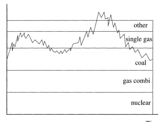
minimum on/off times for generators. The Pool then stacks these bids starting with the lowest price offered (see figure 1-2). It then looks at the predicted demand for the day, and creates a preliminary plan of how much power each generator should be allowed to produce during each hour of the next day. This information is then relayed back to the IPPs. The hourly price of power is determined by the price of the most expensive bid accepted for that specific hour. This price is then paid to all IPPs scheduled to produce in that hour, even if their actual bid was lower. This led to interesting practices such as "zero-bidding", where the IPPs bid very low to ensure their sales. The Pool will send updated signals each hour, telling the IPPs how to set their power output, based on actual demand measurements.

1.2.3 Positive Aspects of the British System

The main attractive features of the British approach to deregulation lies in its security and predictability. The Pool maintains full control over the hourly settings on each generator. Therefore the only major uncertainty comes from the load. Since methods for load forecasting were developed over the years, very little uncertainty is left under

(12)

Load (MW)

other

single gas

coal

gas combi

nuclear

Time

Figure 1-2: Stacking Generation According to Bid Price

normal operating conditions. The use of a single pool also eliminates much of the market power of the large consumers. Since the pool offers a single price on power both on the supply and demand side, industries can no longer negotiate special deals at the expense of small consumers. The result has been that after deregulation electricity prices actually rose for some industrial buyers while they were reduced for individual consumers.

1.2.4 Drawbacks of the British Model

Despite its benefits, several concerns plague the English power pool. The most serious problems are:

1. The Allocation of Generation: One result of the stacking of bids by the Pool, is that the generators whose bids end up close to the base load of the system will be forced to alter their power output frequently during the course of the day. The emergence of cheap, combined cycle gas turbines, has resulted in moving

(13)

the older, coal fueled, plants upwards in the stack, into the region affected by load fluctuations. Coal plants however, are badly suited for quick turn on/off type operation. This leads to additional operating costs which in turn results in an overall increase in the price of electricity. The coal plants would prefer to supply large industrial consumers directly, without being scheduled by the pool. This would give them a lower sales price, but in return they would be guaranteed a steady demand. The Pool and the Grid Company however, do not allow anyone to use the grid for transactions which have not been processed through the Pool. This is an example where the pool system actually inhibits free competition and drives up energy prices.

2. Peak Load Pricing: The stacking system used for pricing can have disastrous effects during extreme peak load periods. If demand rises far above normal, the Pool is forced to consider bids which were never meant to be implemented (such as turning on and shutting off a coal plant within a short time span). Because the IPP does not really wish for the Pool to use its generation in such a dynamic way, his bidding price may be up to ten times the price when load is nominal. Under the agreement between the Pool and the IPP's, if the Pool is forced to accept such a bid it has to pay each producer the price awarded to the most expensive bid. Thus the overall energy price can multiply within minutes even for customers with long term stable contracts. In order to avert this risk, industrial customers are forced to practice what is know as 'hedging'. Essentially, this means that the companies integrate vertically so that they both sell the power to the pool and buy power from it. In reality this is carried out by special power brokers who are hired by risk averse consumers at a brokers fee.

3. No Market for System Regulation: While IPPs can offer bids for normal power production, there is no such system for submitting competitive bids to partici-pate in real-time frequency regulation. The Pool still relies on the old practice of signing expensive contracts with individual generators over long time spans

(14)

to ensure system security.

1.3 The Scandinavian System

The Scandinavian power market became deregulated several years after the British market. This is reflected in a more decentralized model, based on a series of spot markets for trading both regular and control power. The Scandinavian market does not utilize a pool system, but instead allows for bilateral contracts between produc-ers and consumproduc-ers. The remaining imbalances are compensated through the hourly spot market and a market for regulation. For a more detailed description of the Scandinavian market, see [12].

1.3.1 Market Participants

The main market participants are the IPPs, the System Operator, the Power Bro-kers, the Distributors and the Consumers. The system operator is responsible for the maintenance and expansion of the network. He is also responsible for compensating any power losses which occur on his lines. As a result, the system operator is by far the largest consumer of power in the Scandinavian system. The other participants contribute to the process of supply/demand balancing. Which participant is respon-sible for this balance is specified in the contract. Each bilateral contract must specify a balance responsible actor. If this actor does not have access to his own generation (as is the case with a power broker) he must buy or sell power on the spot market in order to balance supply and demand.

1.3.2 The Market

The Scandinavian market is based on bilateral contracts between power producers and consumers. These contracts could take the form of energy contracts, under which the consumer is free to consume power at any rate as long as his total energy consump-tion over the specified time period does not exceed a given amount. Alternatively

(15)

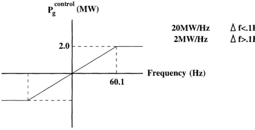
the consumer ccould sign a power contract. These contracts are usually cheaper, but require the buyer to follow a prespecified contract curve for its power consumption. As mentioned above, each bilateral contract must specify the party is balance respon-sible for balancing power in the transaction. The party which is designated as balance responsible will be held financially responsible that demand and supply are perfectly matched. Since the balance responsible actor may not be able, or willing, to change its own production to meet the demand in real time, a spot market has been created where balance responsible parties can trade power on an hourly basis. While a bilat-eral contract specifies which party will be financially responsible for balancing each transaction, the system operator will always be physically responsible for ensuring stable frequency of the entire grid. In order to guarantee the security and stability of the network, the system operator has to assure the availability of sufficient levels of reserve generation for frequency control. In Scandinavia, a separate competitive market has been created for thispurpose. The system operator buys control gener-ation in the form of control packages, effective for three months. IPPs compete for these contracts by submitting a packaged bid of the following form:

1. For frequency deviations less than .1 Hz, supply control generation at the rate of 20MW/Hz

2. If frequency deviates beyond .1Hz, supply 2MW control generation. 3. If frequency deviates beyond .5Hz, supply 3MW control generation.

These contracts effectively provide proportional frequency control for deviations up to .1Hz, and a fixed amount of reserve generation for deviations beyond that. The number of these packages which need to be purchased by the system operator depends on the size and natural response of the grid. In Scandinavia the operator is required to purchase 125 packages for each three month period (see [12] for a detailed derivation of this number). In addition to these long term control offers there exists a half-hourly spot market on which an IPP can sell excess generation or offer to decrease its output in return for compensation from the system operator. In this

(16)

Price

Pspot

,urve

Demand

_MW

Figure 1-3: Spot Market Price Determination

market the system operator determines its total need, then stacks the offers received and eventually pays all accepted offers the same price, equal to the price of the most expensive offer accepted (see figure 1-3).

This spot market can be used by the system operator to deal with extreme devia-tions in frequency, or to improve the performance of the primary level controllers by speeding up the frequency recovery. Scandinavia still lacks an automated system of

allocating this secondary level control generation in an optimal fashion.

1.3.3 Positive Aspects of the Scandinavian Model

1. Flexible Contracts. One great advantage of the Scandinavian model is that it allows the market participants to form bilateral contracts which optimize the benefits for both producers an consumers. The generators can choose a type of contract which suits thier performance potential. A coal fired plant for example would be more likely to offer a low priced contract for a steady supply of power,

(17)

while a combined cycle gas plant would be able to track an erratic consumer at a higher price.

2. Competition for System Regulation. By allowing IPPs to offer competitive bids on controls the Scandinavian market has been able to secure a high level of reserve generation at relatively low prices.

1.3.4 Potential Problems with the Scandinavian Market

One issue which remains unresolved in the Scandinavian market is how to allocate the control generation which is purchased through the spot market. The power is purchased with price as the only consideration, ignoring the position of the generator in the network. While this may be a minor issue in a relatively small market like Scandinavia, it could translate into a real problem in the U.S. power system which consists of a large number of control areas.

1.4 Relevance of the European Experience to the

American Market

Many of the lessons learned in the UK and Scandinavian markets can be directly applied to the American deregulation process. I will try to argue in this thesis that the US has much to gain by following the Scandinavian market structure and adopting a less rigid market structure centered around bilateral contracts. The experience in Europe has shown that attempting to force the market into optimal operating conditions, mainly by dispatching generator output levels, will backfire in the long run since it does not provide value-based compensation for power producers. This results in suboptimal allocation of capital investment which drives the system away from optimal operating conditions. Using direct contracts between suppliers and load, as in the Scandinavian model, creates a transparent market where services are priced solely based on their financial value to market participants. Given the right incentives, the market will automatically adapt itself, through the reallocation of

(18)

generators, to reach a global optimum. The mechanics of this adaptation process will be discussed in depth in a later section. In translating the European deregulation experience to the US, one has to consider a series of characteristics of the American market that clearly sets it apart from its UK and Scandinavian counterparts. The most striking difference is the shear size of the US market. This is not only reflected by the quantitative differences in the amount of power traded, but also in qualitative differences in the structure of the transmission network. I have singled out two key issues which have to be addressed in translating the European models to the United States.

1. Uniform Flow of Power: In both the British and Scandinavian transmission grids, power almost exclusively flows from generators in the north to loads in the southern end of the grid. This characteristic allows system administrators to all but disregard concerns of loop or counter flow in the network. It also greatly simplifies the introduction of high capacity HVDC lines into the sys-tem without upsetting the natural settling effect of the AC network. Finally, a north to south flow of power allows for a simple pricing shceme for transmis-sion, as losses are directly proportional to physical distance of generator and load. The power grid in the United States does not process the luxury of a simple north-south trade of power. As isolated markets throughout the country open up to inter area trade, we can expect a drastic increase in the attempts to move power in all directions across the network. This poses a profound chal-lenge for the system administrators who have to find a fair an effective means of compensating for transmission losses, which now includes the prospect of nega-tive losses due to counterflow. Furthermore they need to consider transmission capacity constraints, which is complicated by the fact that physical power trans-mission is not point to point, but dispersed in accordance with Kirkovs laws. This means that a local transaction of power in one area of the country can affect the availability of transmission capacity on a line hundreds of miles away. Reserving transmission capacity and recovering transmission costs are highly complex tasks which have yet to be fully addressed.

(19)

2. The presence of multiple control areas and system operators: Closely tied to the above discussion of transmission constraints and transmission cost recovery is the question of the future roles of control areas and system operators. In the regulated industry each control area represented isolated markets which inter-acted only through large scale, pre-scheduled, transactions. In the deregulated market however power brokers will seek to take advantage of temporary local price differences by moving power between and across control areas on short notice. In order to accommodate such transactions the system operator must agree on a method for pricing the transmission component of inter-area trades. Currently this is being done by point to point transmission contracts which specify hypothetical contract paths between generators and loads. The network owners located along the contract path are compensated for the transmission service. The physical delivery of the power however will be across a wide va-riety of control areas many of whom are not specified in the contract and are therefore forced to provide their services for free. This system clearly needs to be replaced by compensation based on actual services rendered, or else we risk driving a large portion of transmission providers out of business.

1.4.1 Analysis of the Need for New Modeling to

Accommo-date Deregulation

The drive to decentralize the power market in the United States began as a purely economic endeavor. The people in charge of the technical operations of the network have mostly clung to the old axiom 'the more regulation, the more security'. In this thesis we attempt to take a unified approach to the technical and economical issues involved in shaping a power market. While we recognize that it is not possible to technically outperform a fully coordinated system operation, we intend to show that the increased economic freedom under deregulation provides the system operator with new tools for analyzing and affecting the behavior of other players. The first step in this process is to develop a unified system model which includes the physical

(20)

constraints of the transmission grid as well as the economic feedback provided by dynamic market prices. Such a model will give us a tool necessary to address the vital questions of system stability and performance under competition. It will also allow us to simulate the result of economic as well as technical disturbances under the newly proposed market structures for trading power and control generation. Perhaps the most important point that we wish to get across in writing this thesis, is that any party which intends to be a successful participant in the future American power market will have to shift its focus away from the old paradigm viewing technical and economical issues as separate entities. Instead, in a fully deregulated market, one must learn to skillfully utilize complex technical and economic tools made available by the increase in economic feedback from market participants.

(21)

Chapter 2 A New Market Structure for the

American Electric Power Industry

2.1 Problem Statement

In this chapter we propose a new market structure under which industry participants can trade power, as well as any ancillary system service related to generation or transmission of power, in a near-optimal fashion. Before we begin to describe a possible solution, we need to define the criteria under which such a market structure is to be judged. The following is a list of the most important criteria we addressed in creating this proposal:

System security and performance Any feasible market structure must provide

the tools and incentives for industry participants to ensure system security under normal operating conditions. It must also provide the means to regulate power quality (frequency and voltage) within prespecified margins.

Optimize social welfare This includes minimizing the cost of generation, and

avoid-ing situations in which generators can exert market power to increase profits. The market should also provide a means for a system operator to reduce price volatility if it reaches levels that are harmful to consumers.

(22)

Flexibility The market structure should place as few restrictions as possible on the

types, locations and distances involved in the bilateral agreements signed by industry participants.

Fairness of Compensation The market should ensure that profits are distributed

fairly, prioritizing those who can provide the traded commodity or service at the lowest price.

Fairness of Cost Recovery The system operator should recover any cost incurred

from system control or maintenance in such a manner as to create incentives for industry participants not to cause additional disturbances on the system. While the above points do not constitute an exhaustive list of the demands on a suc-cessful energy market, they provide us with some criteria under which we can compare our proposed bilateral structure to the pool based solutions already in existence. We will attempt to show that while the technical criteria can be equally well met under a pool formation, a bilateral market will create more competition, and greater freedom for generators in allocating their production capacity. This after all was the purpose of deregulation in the first place.

2.2 Industry Structure

In order to best illustrate the impact of the proposed energy market structure, we will use a simplified model of the industry. Participants have been grouped into three categories: Generators, Loads and Independent System Operators. In reality of course there exist actors such as power brokers, who are neither producers nor consumers of power. Since these actors do not have any effect on the net amount of power produced or consumed we will not include them in our model. We do however recognize their impact when addressing the issue of market power in the industry.

(23)

2.2.1 Description of Industry Participants and Their

Re-spective Responsibilities

Generators This group includes all market participants that physically inject power

into the network. In a deregulated industry, generators are purely profit-driven entities. They will set their power output levels to maximize their profits with-out considering overall system security or performance. Clear economic incen-tives are needed to make generators behave in accordance with system needs.

Load Loads include all consumers of power. In our setup a distributor serving a

number of small customers will be modeled as a simple load. Loads are assumed to be inelastic to fast changes in the price of power, so that spot market demand is constant over price for a given time period.

System Operator . The system operator is physically responsible for the security and performance of the system. This includes maintaining generation reserves in the case of generator fallout, and supplying balancing power when system fre-quency deviates from 60Hz. Since the system operator is not allowed to own any generating units, he is forced to become a financial actor on the power market to fulfill these obligations. The cost incurred in regulating system performance is recovered through access charges. It is imperative for the system operator to set these charges in a discriminatory manner so as to provide incentives for loads and generators to minimize the disturbance they inflict on the system.

2.3 Physical Model

The model in this section is derived from the structure based model of large electric power systems. We assume the presence of primary frequency control consisting of a governor-turbine-generator set. The primary control responds to differences in the reference frequency setting on the governor form the actual system frequency. The secondary level control which we address in this paper deals with how to set the reference frequency on the generators to maintain a stable system frequency. The

(24)

linearized dynamic model for system frequency takes on the form:

wG[k + 1] = (I - uKpT)wG[k] + (I - aD)Bu,[k]

+ af[k] - aDpds[k] (2.1)

where a = - [ is a diagonal matrix representing generator droop constants, I

is an identity matrix, D stands for a diagonal matrix whose terms are damping coeffi-cients of generators, u,[k] - wf [k + 1] - wf [k] is secondary (AGC) control signal at

the discrete instant kT, vector f [k] = F[k

+

1] -F[k] is a vector of incremental tie-line flows into a control area (for an isolated system this vector is identically zero) and

d[k] = XL[k + 1] - XL[k] is vector of incremental deviations in real power of loads.

Matrices Kp and Dp are function of electrical characteristics of the transmission grid. The corresponding linear model for the power output at each generator is of the form:

Xc[k + 1] (I - KpaTs)XG[k] + Kp(I - aD)Tswrf[k]

--a(f[k] - Dpd[k]) (2.2)

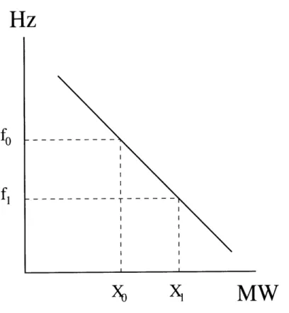
The generators will use equation (2.2) to set the refernce frequency on their gov-ernors so that their output corresponds to the expected behavior of the load (i.e. the contract curve). If we load at equation(2.1) this means that if XL[k] moves along the contract curve, then the effects of u,[k] and d,[k] will cancel each other out and there will be no net deviation in frequency. However, any unscheduled fluctuation in the load will translate into a proportional offset in system frequency. The magnitude of the frequency deviation will depend on the electrical characteristics of the transmis-sion grid. For an isolated network, we can simplify this relationship to take on the form:

(25)

where,

Ximbalance[ k] = Xscheduled[k] - XL (2.4) Equation (2.3) assumes that generators set their reference frequencies so that their output level will be equal to the scheduled demand. Note that the actual output of the generator will not necessarily correspond to the scheduled levels. This is because of the so-called quasi-static droop characteristic which relates real power output, system

frequency and governor frequency setting.

WG[k] = (1 - od)w f[k] - uP[k] (2.5)

Equation (2.5) tells us that if the reference frequency is kept constant while system frequency increases, then the real power output of the generator will decrease. This serves as and automatic correction system for the network, guaranteeing that actual load and generation will always match in real time. It is because of this droop characteristic that we are defining the disturbances on the system to be the difference between scheduled generation and actual load. From here on when we address the issue of purchasing balancing power, from the spot market or the controls market, we will be referring to buying scheduled power as reflected by the reference frequency settings.

Returning to equation (2.3), this relationship gives us a direct measure of the amount of balancing generation needed to restore frequency to nominal. Specifically, if frequency has deviated by wo, the necessary amount of control generation is given

by:

Xcontrol = (1/d)wo (2.6)

Equation (2.6) in fact gives us the form of a simple proportional control law to maintain nominal frequency. This relation translates nicely into the interconnected system, where the constant 1/d represents the degree of responsibility of the control area towards regulating overall system frequency. We will further discuss the

(26)

impor-Hz

Sx

MW

Figure 2-1: Natural Frequency Response of an Isolated System

tance of this relation when we address the physical implementation of the controls market.

fo

f,

(27)

Chapter 3 Temporal and Functional Division

of Power Markets

According to the market structure we are proposing, power can be traded in three different contexts: on the long term market, the spot market, and the controls market. The contracts associated with each of these markets differ both in time span and pricing structure. Below is an outline of their most important characteristics.

3.1 Long-Term Market

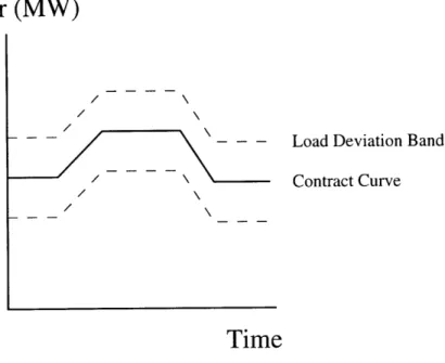
Trade on the long term market is strictly bilateral. A generator signs a contract directly with a consumer. This contract includes a contract curve, specifying the scheduled rate of production and consumption at any instance during the duration of the contract. Since the consumer cannot be expected to forecast his consumption exactly, and since the generator will be unable to track fast load fluctuations in real time, the contract also specifies a band around the contract curve inside which load and generation are allowed to deviate without being penalized. This produces a bounded contract curve shown in figure 3-1.

The generator will register this contract with the system operator, who uses the magnitude of the allowable generation to determine access fees. The loser the bound, the higher the access fee. This is a technically sound criterion, since the bound

(28)

repre-Power (MW)

Time

Figure 3-1: Structure of Long-Term Contracts

sents the maximum mismatch between load and generation. When such a mismatch occurs, the system operator has to provide balancing generation. He recovers the cost thereby incurred through the access fees. By setting the access fees in an individ-ualized manner, the system operator gives generators an incentive to minimize the width of their contract bounds. Setting the bounds to narrow however could results in significant penalties if the load deviates outside the allowed margins. If access fees and penalties are set accordingly, the width of the bounds specified in the contract should provide an accurate measure of the actual volatility of the load. This informa-tion can in turn be used by the system operator to estimate the maximum cumulative disturbance on his system. Using this estimate he can then decide how much control generation to reserve for future time intervals.

3.2 Spot Market

Power on the spot market is traded in one-hour intervals. Before the start of each hour generators enter bids specifying the quantity of power they are offering and the price they are demanding. A generator may divide the power he intends to sell into many smaller bids, so that he can effectively offer a bid curve, as shown in figure 3.

Load Deviation Band Contract Curve

(29)

This allows a generator to bid his own marginal cost curve, if he so desires.

The demand from the spot market is generally made up of the system operator, who uses this power to compensate for system losses and generation/load mismatches. However generators may also buy power from the spot market if they cannot cover their long term contracts with their native generation. Once spot market demand has been determined, the generator bids are stacked starting with the lowest price. The point at which the stack of bids intersects the cumulative load specifies the clearing price, defined as the price demanded by the most expensive bid accepted. This price will be awarded to all accepted bids.

3.3 Controls Market

This market offers an alternative source of balancing generation for the system oper-ator. Generator bids are in the form of an obligation to alter their power output in response to frequency deviations. For example a bid could take the form:

Xcontro = k AF forAF < AFmax (3.1)

Xcontrol = kAFmax forAF > AFmax (3.2)

(3.3)

The system operator effectively pays the generator to maintain a control reserve. By deciding how many of these bids to accept, the system operator determines the size of the control reserve for his area. This decision will be closely linked to the maximum anticipated disturbance defined by the by the sum of the bounds on the long term market. The system operator may choose the accept enough bids to cover to match his control reserve with the sum of the long term bounds, or he may rely on the spot market to pick up any additional imbalance on his system. The decision on how much control reserve to maintain has a profound effect on the price volatility of the spot market. We will quantify this relationship, and discuss the possible strategies

(30)

control P (MW) 2.0 20MW/Hz A f<.lHz 2MW/Hz A f>.lHz Frequency (Hz) 60.1

Figure 3-2: Structure of Contracts Traded on the Controls Market of the system operator in a later section.

3.4 Modeling of Economic Decision Making

Pro-cess

Each generator in the network is faced with the decision of how much of his production capacity to allocate for sale on each of the available markets. In order to make an informed decision, the generator needs a means of evaluating expected profits of each scenario. He also needs to account for the risk factor associated with reserving his capacity for sale on the short-term market. In this section we derive the expressions for the expected profits on each of the markets, and show the conditions that must be met for the overall system to be in economic equilibrium. Once we have modeled how generators enter the market, we can proceed to show how physical disturbances translate into deviations in market price.

3.4.1 Assumptions Related to Generator Behavior

The following assumptions were made in modeling the behavior of power producers: 1. Generators are purely profit-driven. They will not act in the interest of system security or performance unless they are given clear financial incentives to do so.

(31)

2. Generators have no market power. They are price takers on all markets. 3. Demand is inelastic to fast price changes on the spot market.

4. All power producers have smooth quadratic cost curves, and consequently lin-early increasing marginal costs. We model these as:

TotalCost = aX2 + b (3.4)

MarginalCost = 2aX (3.5)

3.4.2 Profits Under Long-term Contracts

When a generator enters into a long-term contract he obligates himself to sell power at a rate given by the contract curve and at a prespecified price. In doing so he eliminates any risk of not being able to sell his power, but also robs himself of the ability to take advantage of short term price peaks on the spot market. Since generators are assumed to be price takers, the profit associated with selling on the long-term market is easy to calculate. Faced with a price PL, the generator will set his total power output so that his marginal cost is equal to PL.

PL = 2aX (3.6)

Using this constraint we can express the total profits of the generator in terms of long-term price.

IL = PF/4a (3.7)

Since the long term price is known in advance, there is no risk involved in this contract, and we can view (3.7) as a guaranteed profit.

(32)

3.4.3 Profits under Short Term Contracts

We will now consider the case of the producer who decides to reserve all his production capacity for sale on the spot market. Again we assume that the generator is a price taker, who at each hour will see a new spot market price (Ps). At this price the market will absorb any amount power he can generate. As in the long-term case, the producer will maximize his profits by setting his power output to a level such that the marginal cost of generation is equal to the current spot market price. For each discrete spot market interval the profit of the power producer will then be given by:

-I[k] = Ps[k]/4a (3.8)

If the spot market price was pre-determined, the producer could simply sum the projected profits over each discrete interval, given by (3.8), compare them to the profit on the long term market (3.7), and thus decide where to place his production capacity. In reality however the spot market involves a great deal of uncertainty. Countries who have undergone deregulation have experienced a considerable increase in price volatility on the short-term market. In order to allocate production capacity between the long term and spot market, the producer needs to generate an estimate of his expected profit on each market. To achieve this we will model the spot market price as a random variable Ps[k], with expected value Us [k], and variance ' [k]. Using equation (3.8) we can now express the expected profit in terms of the characteristics of this random variable.

E{Profit} = E{Ps[k]2/4a} = Us[k]2/4a + or/4a (3.9)

So what does this expression tell us about the effect of price volatility on the spot market? If we compare equation (3.15) to our expression for profits on the long-term market (3.7), we find that they have a similar form. Indeed if we set the expected price level Us[k] on the spot market equal to the actual long term market price we find that the expressions for profits on the markets are identical with the exception of the term ua/4a on the spot market. This factor is a direct result of that the profit

(33)

is a nonlinear function of price, in this case a simple quadratic function. A marginal increase in spot market price will therefore create a large increase in overall profits, while an equivalent decrease in price will cause a smaller decrease in profits. As a result, an increase in the price volatility (i.e. larger a') will result in greater expected profits on the spot market, as predicted by (3.15). In an industry where participants choose between investing only on the long-term market or only on the spot market, the equilibrium will be reached when expected profits are equal on both markets. Since price variance is always positive, this can only occur if the expected value of the spot market price is below the actual long-term price. This price differential can be expressed directly as a function of spot market price volatility.

P = U2 + r (3.10)

The result predicted in (3.10) seems counterintuitive. It is important to realize that the above model does not take into consideration that most generators are likely to be risk adverse. If we would include this behavior in our modeling we would have to add a negative risk correction term to the right hand side of equation (3.10). As it stands, the model simply reflects the effect of passing an uncertain price signal through a nonlinear system.

3.4.4 Mixed Strategy Solutions

The above analysis will allow us to find equilibrium prices under the condition that each generator uses a pure strategy of selling only on the long-term market or only on the spot market. In reality there is nothing to prevent a producer from dividing his output between the two markets. In order to specify the long and short term supply curves, we first have to determine under which conditions it is profitable for a producer to be selling on both markets. Consider the following example. A producer with marginal cost MC = 2aX sees a long-term price PL. He therefore commits a capacity of XL = PL/2a to the long-term market, setting long term price equal to long term marginal cost. During the course of the long-term contracts, the producer

(34)

notices that the short-term price increases above the level of his current marginal cost

(PL). He can now increase his profits by selling power on the spot market until the

marginal cost of production is equal to the spot market price. The same is true for all generators who sell power on the long-term market.

3.5 The Spot Market Supply Curve

We will now proceed to derive the supply curve for the spot market of a simple generic system. Assume our system contains a total of N generators. Each generator has a marginal cost curve of MC = 2aX. Further assume that of all producers, a subset of M generators decide to reserve all their capacity for sale on the spot market. The remaining N-M generators will sell power according to the mixed strategy described in the previous section. We derive the shape of the supply curve by considering two separate instances:

1. For Ps < PL, the spot market will be supplied only by the subset of M generators. Under these conditions the supply curve is given by:

Ps = 2aX/M (3.11)

2. For Ps > PL, all generators in the system will supply power to the spot market. This will reduce the slope of the supply curve by a factor of N/(N-M). Combining this change of slope with the curve described in (3.11), the total supply curve for the spot market takes on the form:

Ps = 2aX/M forPs < PL (3.12)

Ps = (1 - M/N)PL + 2aX/N forPs > PL (3.13)

(3.14)

(35)

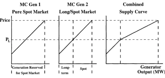
MC Gen 1 MC Gen 2 Combined Pure Spot Market Long/Spot Market Supply Curve Priep ---

---

----I I I l- ... - I- I -I I I I I I I I II I 1..

IGeneration Reserved I ILong- Spot I Generator

I for Spot Market I I term I I Output (MW)

Figure 3-3: Two-Slope Supply Curve

As seen in the figure, we are dealing with a two-slope supply curve. The breaking point coincides with the price level where generators committed to long-term contract begin to enter the spot market.

3.6 Effect of Supply Curve on Price Volatility

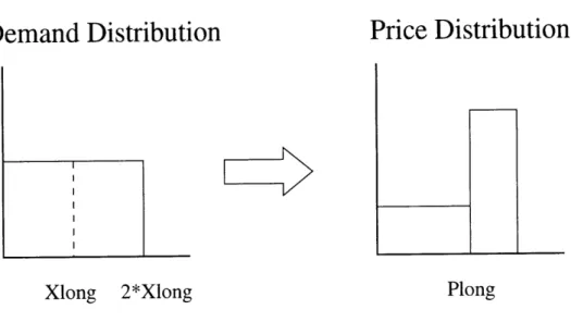
The reason we have gone through such length in deriving the structure of the supply curve is that it represents the link between the physical and economic processes modeled above. In the short term, the system is driven by physical disturbances in the form of generator/load mismatches. Such disturbances translate directly into spot market demand. The shape of the supply curve tells us how this demand will cause movements in spot market price. In effect the supply curve is a transfer function between the physical and economic disturbances on the system. Let us use a simple example to illustrate the effects of the supply curve on price volatility and generators profit levels. Assume the supply curve is of the form described in equation (3.14), and the physical disturbance (Xd) is a random variable evenly distributed between zero and (M/a)PL). Figure (3-4) shows how the resulting distribution of spot market price is weighted by the supply curve.

Note how the distribution of the disturbance was selected so that it fell symmetri-cally around the breaking point of the supply curve. When we examine the resulting distribution of the spot market price we find that it no longer displays this symmetry.

(36)

Demand Distribution

Price Distribution

Xlong 2*Xlong Plong

Figure 3-4: Effect of Supply Curve Shape on Prive Distribution

While spot price is equally likely to above or below the long-term price level, the range of the deviation is significantly smaller for price levels above PL. On a system-wide level, this means that price is more volatile in the lower price ranges, and that we are less likely to experience extreme price peaks. This illustrates one of the advantages of the proposed market structure. By not restricting balancing generation to a few selected generators, we avoid having high price volatility in the upper price ranges, avoiding unreasonable peaks in spot market price that could be extremely destruc-tive for the end consumer. If we examine these results from the perspecdestruc-tive of the individual generator, we find that it has a significant impact on how the producer allocates his resources between the long and short-term markets. In modeling the profits on the spot market, we found that due to the nonlinear relationship between spot market price and producer profits, the expected profits actually increased as the price became more volatile.

E{Profit} = E{Ps[k]2/4a} = Us[k]2/4a + ao/4a (3.15)

The shape of the supply curve however is telling us that even if the demand to the spot market is extremely volatile, this will not necessarily translate into high price peaks. The incorporation of long term generators into the spot market therefore has a distinctly negative effect on the projected profits of the purely short term producers.

(37)

Reduced profits on the spot market will cause generators to reevaluate their allocation decisions, causing more producers to enter into long term contracts. This will change the shape of the spot market supply curve by moving the breaking point to left, increasing the slope of the primary segment.

Since the price level of the new supply curve is higher than the old for any given demand, the generators which chose to remain with the pure spot market strategy will see an increase in their profits. Market actors will continue to reevaluate their strategies until an equilibrium is reached where expected profit levels for both strate-gies are equal. This equilibrium will shift as new generators enter the market, or as the characteristics of the load changes. The process by which the market responds to such changing conditions is outlined step by step below.

1. The Power Producers decide how to allocate their generation capacity between the spot market and long term market. Their decisions are based on a known long-term price and an estimate of how the spot market price is going to behave. This in turn determines the shape of the spot market supply curve.

2. Fast fluctuations in load causes power imbalances on the system which translate into demand for short terms balancing power. This power must be purchased by the System Operator on the spot market.

3. The change in demand for spot market power translates into a fluctuation in the spot market price. The magnitude of the price change given a deviation in demand will depend on the shape of the spot market supply curve.

4. Increased volatility in spot market prices will increase the profit incurred by generators investing their capacity in this market. If the volatility remains high during the cause of the long-term contract period, more generators will enter the spot market during the next period, and we are back at stage 1. Thus we have closed the loop, and shown how the system can adjust itself until it reaches a stable equilibrium.

(38)

Chapter 4 Simulation

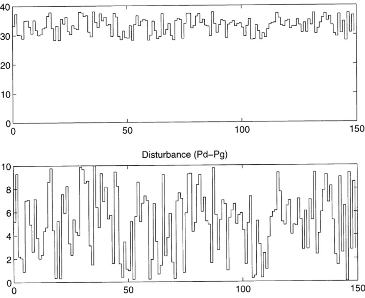
We will now attempt to demonstrate the adaptive behavior of market participants by simulating a small system under realistic conditions. The system consists of five identical generators, and is driven by a single, cumulative, stochastic load.

Generator Characteristics Each generator has a total production capacity of 10

units of power. The cost curve is given by C = X2+ 4X + 2, yielding a marginal cost curve of MC = 2X + 4.

Load Characteristics The load consists of a fixed base portion of 28 units, and a

stochastic portion with probability density function evenly distributed between zero and ten for each discrete step. The base portion is covered by long term contracts which are renewed every 50 time steps. The stochastic portion repre-sent unpredicted load variations for which the system operator must compensate by purchasing balancing power on the spot market.

(39)

Total System Load

I Ip-~v

100

Disturbance (Pd-Pg)

50 100

Figure 4-1: Simulation Results

40 30 20 0 150 150 E F

(40)

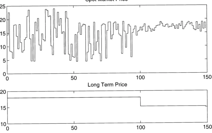
Spot Market Price 25 20 15 10 5 0'-20 15 10 0 50 100 150

Figure 4-2: Simulation Results

0 50 100 150

(41)

Average Price

50 100

Total Cost of Generation

50 100

Figure 4-3: Simulation Results 20 19 18 17 16 15_I0 0 150 500 450 400 350 300 20 0 150

(42)

4.1 Analysis of Generator Behavior for each Time

Sequence

4.1.1 Sequence A: Time 0-50

We have chosen an arbitrary starting point from which the market can evolve. Gen-erators one through four have committed generation to the long term market, each supplying a load of seven units. The long term market price, given by the marginal cost of generation, is 18. The fifth generator has chosen to participate only in the spot market.

4.1.2 Sequence B: Time 50-100

Long term contracts are allocated as in A. Generators one through four now decide to offer their excess generation for sale on the spot market when spot market price exceeds long term prices. Generator five behaves as in A.

4.1.3 Sequence C: Time 100:150

Faced with diminishing profits, Generator five decides to enter the long term market. This decreases the long term demand seen by each of the other generators. Each now supplies a load of 5.6 units, driving the long term market price down to 15.2. The spot market is now supplied soly through excess capacity not used to fulfill long term obligations.

4.2 Analysis of Simulation Results

If we examine the price plots from the simulated system we find several interesting trends. First if we look at the plot of spot market price, we find that the market adapts itself to reduce price volatility. As we move from sequence A to B, we remove the the price peaks on the spot market. This is because we have moved from a steep single slope supply curve to a two slope supply curve. As we enter sequence C, the

(43)

downward volatility off spot market price dissapears. This is a result of all generators participating in the long term market. There will therefore be no one willing to supply the spot market when price is below long term price levels. In addition to reducing price volatility this trend will of course raise the average spot market price. This effect however is overpowered by the simultaneous decrease in the long term price, so that we see a drop in the overall per unit price of power. The trend of the market is towards a decrease in average price and a reduction of price volatility. If we examine the overall cost of production we find a similar trend. The total cost of production for sequence A is 1,873. It drops to 1,8488 for sequence B, and falls further to 1,777for sequence C.

4.3 The Impact of the Controls Market

In the simulation presented in the previous section, we demonstrated how generators adapted their strategies of sale between the spot and long-term markets to minimize overall cost of production, even when faced with a stochastic load. In theory it would be possible for the system operator to rely solely on the spot market for balancing generation. Because of security concerns however it would be advantageous if one could guarantee the presence of balancing power capacity through long term contracts. This is the role of the controls market, which we briefly described earlier and will now revisit in the context of system operator strategies for optimizing production allocation and reducing price volatility.

4.3.1 General Structure of Controls

While the specific implementation of the control process differs from country to coun-try or even from one control area to another, there are three basic temporal steps which are always present.

Forecasting The pool operator attempt to predict the cumulative load curve for his

Closed-loop market dynamics for a deregulated electric power industry

Closed-loop Market Dynamics for a Deregulated

Electric Power Industry

by

Petter L. Skantze

Submitted to the Department of Electrical Engineering and

Computer Science

in partial fulfillment of the requirements for the degree of

Master of Engineering in Electrical Engineering and Computer

Science

at the

MASSACHUSETTS INSTITUTE OF TECHNOLOGY

Febuary 1998

©

Petter L. Skantze, MCMXCVIII. All rights reserved.

The author hereby grants to MIT permission to reproduce and

distribute publicly paper and electronic copies of this thesis

in

rant

APR 1A2 1999

LIBRARIES

the right to do so.

Department of Electrical Engineering and

Certified by..

...

Computer Science

Febuary 4, 1998

Marija Ilic

Senior Research Scientist

/

Accepted by...

Arthur C. Smith

Chairman, Department Committee on Graduate Students

Closed-loop Market Dynamics for a Deregulated Electric

Power Industry

by

Petter L. Skantze

Abstract

Acknowledgments

Contents

List of Figures

Chapter 1

Analysis of Market Structures

Under Deregulation

1.1

Introduction

1.2

The British System

1.2.1

Market Participants

1.2.2

The Trading Process

1.2.3

Positive Aspects of the British System

Load (MW)

other

single gas

coal

gas combi

nuclear

Time

1.2.4

Drawbacks of the British Model

1.3

The Scandinavian System

1.3.1

Market Participants

1.3.2

The Market

Price

,urve

Demand

MW

1.3.3

Positive Aspects of the Scandinavian Model

1.3.4

Potential Problems with the Scandinavian Market

1.4

Relevance of the European Experience to the

American Market

_MW