Classification of whole brain fMRI activation patterns

Classification of Whole Brain fMRI Activation

Patterns

by

Serdar Kemal Balci

Submitted to the Department of Electrical Engineering and Computer

Science

in partial fulfillment of the requirements for the degree of

Master of Science in Electrical Engineering and Computer Science

at the

MASSACHUSETTS INSTITUTE OF TECHNOLOGY

September 2008

@

Massachusetts Institute of Technology 2008. All rights reserved.

Author

...

Department of Electrical Engineering and Computer Science

August 29, 2008

Certified by ...

...

...

Polina Golland

Associate Professor

Thesis Supervisor

Accepted by

Chairm•

j0CT

222008

---•---

ARCHIVES

Terry P. Orlando

in, Department Committee on Graduate Theses

MASSACHUSiETTTS INSTITUTE OF TECHNOLOGY I

CT 2 2 2008I

Classification of Whole Brain fMRI Activation Patterns

by

Serdar Kemal Balci

Submitted to the Department of Electrical Engineering and Computer Science on August 29, 2008, in partial fulfillment of the

requirements for the degree of

Master of Science in Electrical Engineering and Computer Science

Abstract

Functional magnetic resonance imaging (fMRI) is an imaging technology which is primarily used to perform brain activation studies by measuring neural activity in the brain. It is an interesting question whether patterns of activity in the brain as measured by fMRI can be used to predict the cognitive state of a subject. Researchers successfully employed a discriminative approach by training classifiers on fMRI data to predict the mental state of a subject from distributed activation patterns in the brain. In this thesis, we investigate the utility of feature selection methods in improv-ing the prediction accuracy of classifiers trained on functional neuroimagimprov-ing data.

We explore the use of classification methods in the context of an event related func-tional neuroimaging experiment where participants viewed images of scenes and pre-dicted whether they would remember each scene in a post-scan recognition-memory test. We view the application of our tool to this memory encoding task as a step toward the development of tools that will enhance human learning. We train sup-port vector machines on functional data to predict participants' performance in the recognition test and compare the classifier's performance with participants' subjective predictions. We show that the classifier achieves better than random predictions and the average accuracy is close to that of the subject's own prediction.

Our classification method consists of feature extraction, feature selection and clas-sification parts. We employ a feature extraction method based on the general linear model. We use the t-test and an SVM-based feature ranking method for feature se-lection. We train a weighted linear support vector machine, which imposes different penalties for misclassification of samples in different groups. We validate our tool on a simple motor task where we demonstrate an average prediction accuracy of over 90%. We show that feature selection significantly improves the classification accuracy compared to training the classifier on all features. In addition, the comparison of the results between the motor and the memory encoding task indicates that the classifier performance depends significantly on the complexity of the mental process of interest. Thesis Supervisor: Polina Golland

Acknowledgments

I would like to thank to everybody who helped me to prepare this thesis. First, I would like to thank to my research advisor Polina Golland. She provided me a great environment in which research was a fun activity for me. She encouraged me to tackle challenging problems and put endless efforts in teaching. Without her guidance and company I would not finish my thesis.

I would like to thank to all my lab mates in medical vision group: Mert Sabuncu, Thomas Yeo, Wanmei Ou, Danial Lashkari, Bryce Kim and Archana Venkataraman. They always have been of great help to me and I am proud of being a part of this wonderful research group.

I would also like to thank John Gabrieli, Susan Whitfield-Gabrieli, Julie Yoo and Satra Ghosh in providing me with the exciting functional neuroimaging dataset from the memory encoding experiments.

This thesis was in part supported by the NIH NIBIB NAMIC U54-EB005149, NAC P41-RR13218 and the NSF CAREER 0642971 grant.

Lastly, I thank to my parents Servet Balci and Emine Balci and my sisters Zeynep Balci and Giilgah Balci for their boundless support in my life.

Contents

1 Introduction 13

2 Background 17

2.1 Functional Magnetic Resonance Imaging . ... 17

2.2 fM RI Analysis ... ... . . 18

2.3 Classification of fMRI data ... ... 19

3 Methods 23 3.1 Feature Extraction ... 23

3.2 W eighted SVM ... 24

3.3 Feature Selection ... 28

3.3.1 Feature Selection based on t-statistics . ... 32

3.3.2 SVM-based Feature Selection ... 32

3.4 Evaluation Methods ... ... 33

4 Experimental Evaluation 37 4.1 fMRI Experiments and Data ... 37

4.2 M otor Task . . . .. . . . .. . . . .. . . . . 38

4.3 M emory Task ... ... 42

4.3.1 Effects of the Training Set Size . ... . . ... . . . 47

4.3.2 Effects of Spatial Smoothing . ... 47

4.3.3 Feature Selection Effects ... 51

4.4 Sum m ary . . . .. . .. . . . .. . 55

List of Figures

3-1 Threshold selection procedure used for feature selection based on the

t-statistics ... .. ... .. 31

3-2 The procedure for the SVM-based feature selection. . ... 33

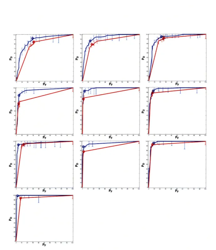
4-1 ROC curves for the motor task for 10 subjects. Red curves correspond to training the classifier on all features. Blue curves correspond to training the classifier using feature selection. Circles show the

operat-ing points correspondoperat-ing to min-error classification accuracy. ... 39

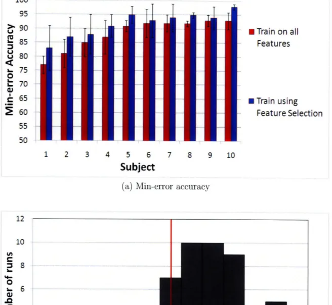
4-2 (a) Min-error classification accuracy for the motor task for 10 subjects. (b) The histogram of the increase in classification accuracy when using feature selection. The horizontal axis shows the percentage difference in the min-error classification accuracy between using feature selection and training the classifier on all features. The area under the curve equals to the total number of functional runs in the data set, five runs

for 10 subjects. ... . ... ... 40

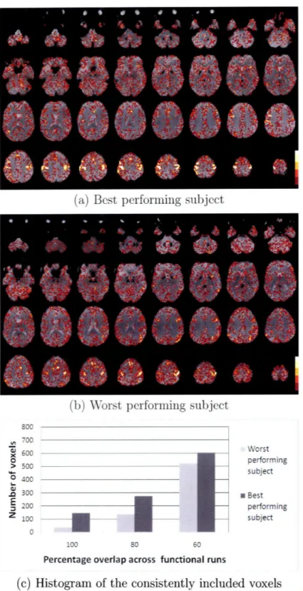
4-3 Feature overlap maps for the best (a) and the worst (b) performing subjects for the motor task. For all five functional runs feature selection is performed on each run. The color indicates the number of runs in which a voxel was selected. Dark red color shows the voxels selected only in one run and white color displays voxels selected in all runs. The histogram (c) shows the number of consistent voxels for the best (dark-gray) and the worst (light-(dark-gray) performing subjects. The number of voxels included in 100%. 80% and 60% of the functional runs are shown. 41

4-4 ROC curves for memory encoding experiment for 10 subjects. Crosses represent subject's prediction accuracy. Blue curves correspond to strategy 1, using the training set for feature selection. Red curves cor-respond to training the classifier only on correctly predicted samples (strategy 2). Green curves correspond to strategy 3, including test set in feature selection. Circles show the operating points corresponding

to min-error classification accuracy. ... ... 43

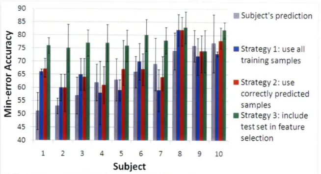
4-5 Min-error classification accuracy for the memory task for 10 subjects. 44

4-6 Feature overlap maps for the best (a) and the worst (b) performing subjects for the memory task. The histogram (c) shows the number of consistent voxels for the best (dark-gray) and the worst (light-gray)

performing subjects ... 45

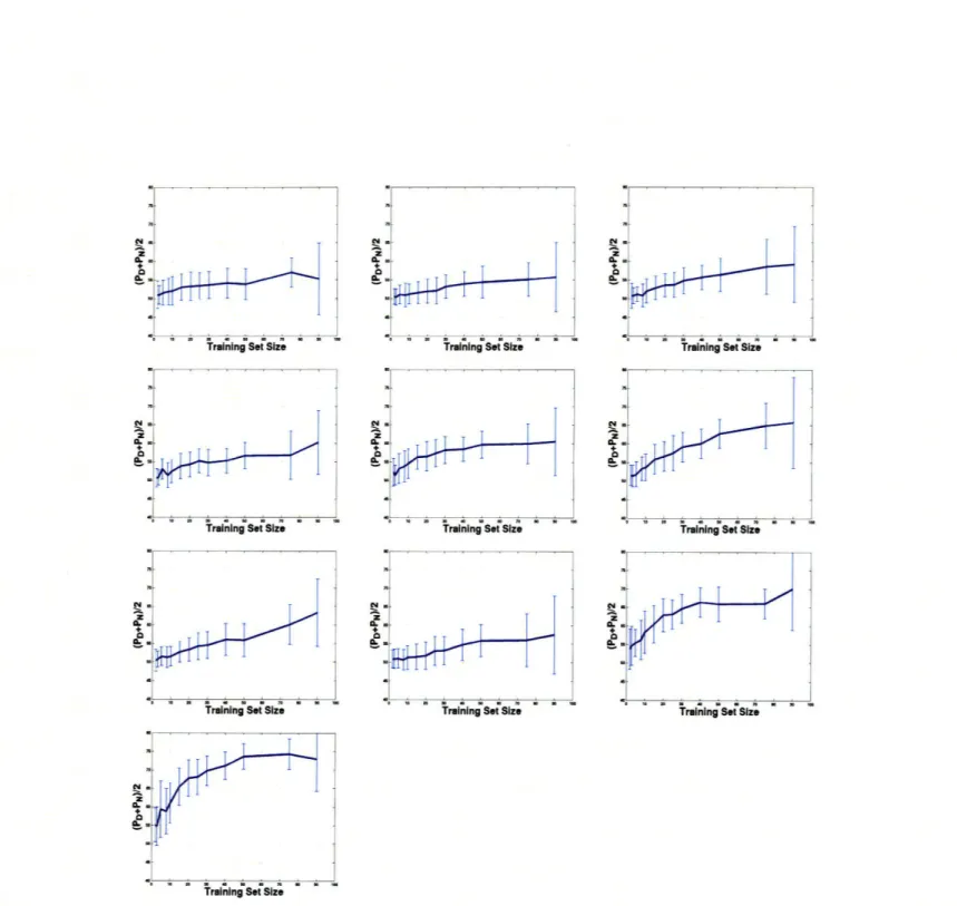
4-7 Learning curves for the memory task for 10 subjects. The mean of the prediction rate on the positive and the negative examples are shown

for varying training set size. ... .. 48

4-8 The effects of spatial smoothing on the classification accuracy. ROC curves corresponding to smoothing (blue) and not smoothing (red) the

data in the pre-processing step are shown. . ... 49

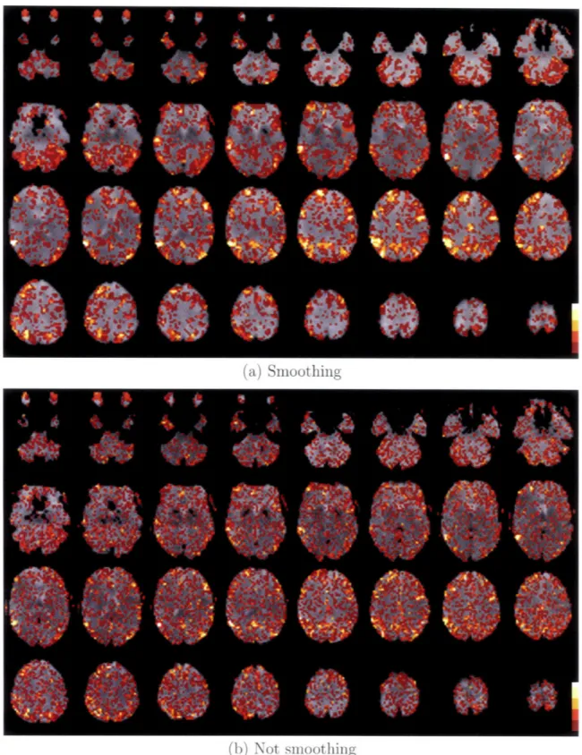
4-9 Feature overlap maps corresponding to smoothed data (a) and not smoothed data (b) for the best performing subject for the memory task. 50 4-10 ROC curves for different feature selection methods for the memory

task. Crosses represent subject's prediction accuracy. ROC curves for using t-test (blue) and SVM-based feature selection (red) are shown. Green curves correspond to using an expert map provided by neurosci-entists. Circles show the operating points corresponding to min-error

classification accuracy. ... 52

4-11 Min-error classification accuracy for different feature selection methods

4-12 Feature overlap maps for different feature selection methods: t-test (a), SVM-based feature selection (b) and expert map (c). A fixed threshold

Chapter 1

Introduction

Functional magnetic resonance imaging (fMRI) is an imaging technology which is primarily used to perform brain activation studies by measuring blood oxygen level dependent signal, which serves as an indicator of neural activity in the brain [25]. Univariate techniques, such as generalized linear model (GLM) [20], are traditionally used to identify neural correlates in fMRI data. Recently, the neuroscience com-munity has been focusing on the thought-provoking problem of whether patterns of activity in the brain as measured by fMRI can be used to predict the cognitive state of a subject. Researchers successfully employed a multivariate discriminative ap-proach by training classifiers on fMRI data to predict the mental states of a subject from distributed activation patterns in the brain [19]. It is an interesting question whether the prediction accuracy of these classification methods can be improved using feature selection methods. In this work, we employ feature selection methods with classification algorithms and apply these methods to a challenging memory encoding experiment.

Predicting the outcome of a memory encoding task is a noteworthy problem, as an important part of human learning is to evaluate whether information has been successfully committed to memory. Humans with superior judgments of learning are shown to perform better in learning tasks [16]. A superior judgment of learning al-lows the allocation of cognitive sources so that information that has been sufficiently learned is no longer studied. Recent functional neuroimaging studies identified brain

regions correlated with actual and predicted memory encoding using univariate anal-ysis techniques[40]. In this thesis, we adopt the discriminative approach to predicting successful encoding from functional neuroimaging data. We view this work as a step toward the development of tools that will enhance human learning. One of the pos-sible applications is human-machine interfaces which employ a feedback mechanism to ensure successful acquisition of skills in critical applications.

In this thesis, we explore the use of classification methods in the context of an event related functional neuroimaging experiment where participants viewed images of scenes and predicted whether they would remember each scene in a post-scan recognition-memory test. We train support vector machines on functional data to predict participants' performance in the recognition test and compare the classifier's performance with participants' subjective predictions. We show that the classifier achieves better than random predictions and the average accuracy is close to that of the subject's own prediction.

Our classification method consists of feature extraction, feature selection and clas-sification parts. We employ a feature extraction method based on the general linear model [43]. We use the t-test [34] and a support vector machine (SVM) based feature ranking method [32] for feature selection and compare their accuracy on our data set. As in our data sets, the class sizes are unbalanced by a factor of about three-to-one, we train a weighted linear SVM, which imposes different penalties for misclassification

of samples in different groups.

In our experiments, we use two data sets, where we validate our method on a simple motor task and evaluate it on the more challenging memory encoding task. In the motor task experiment we demonstrate a highly accurate average prediction accuracy of over 90%. We also provide experimental evidence that feature selection significantly improves the classification accuracy compared to training the classifier on all features. In the memory encoding task experiments we explored the challeng-ing nature of the experiment by varychalleng-ing different components of the system: trainchalleng-ing strategy, size of the training set, the amount of smoothing and the feature selection method. We show that the classification accuracy can be increased by training the

classifier on reliable examples determined using the subject's predictions. We observe that smoothing increases the consistency of selected features without significantly af-fecting the classification accuracy. We also show that multivariate feature selection does not significantly improve on univariate feature selection. In addition, the com-parison of the results between the motor and the memory encoding task indicates that the classifier performance depends significantly on the complexity of the experimental design and the mental process of interest.

The contributions of this thesis include:

* The use of classification algorithms in predicting mental states from functional neuroimaging data. Experimental results on a challenging memory encoding task.

* An investigation of the utility of feature selection methods in fMRI pattern recognition problems.

* A discussion on practical issues arising in training a classifier on fMRI data, e.g. unbalanced data sets, the amount of smoothing, choosing feature selection parameters and whether subjects' responses should be used to find a reliable subset of training examples.

This thesis is organized as follows. In the following chapter we provide a short background on fMRI and review previous work. In Chapter 3 we present our approach to the pattern based classification of fMRI data. We explain the methods used for feature extraction, classification, feature selection and the experimental evaluation setup. In Chapter 4 we describe our data sets and present the experimental results on the memory encoding and the motor tasks. We conclude our thesis with a discussion of our experimental results and point to future research directions in Chapter 5.

Chapter 2

Background

2.1

Functional Magnetic Resonance Imaging

Functional magnetic resonance imaging (fMRI) is an imaging technology which is primarily used to perform brain activation studies by measuring neural activity [25]. For a more comprehensive introduction to fMRI we refer the readers to [37]. fMRI is a popular imaging tool in neuroimaging experiments as it does not involve radiation, is non-invasive, has high spatial resolution and is relatively easy to use. In neuroscience, fMRI has been an important tool for the investigation of functional areas that govern different mental processes, including memory formation, language, pain, learning and emotion [6, 7].

fMRI measures the magnetic properties of blood in the brain with respect to a control baseline. The magnetic properties of blood depends on the degree of oxy-genation level: haemoglobin is diamagnetic when oxygenated but paramagnetic when deoxygenated. In the brain, the degree of oxygenation level in the blood depends on the neural activity. fMRI measures this blood oxygen level dependent (BOLD) signal and this BOLD signal serves as an indicator of neural activity.

Relative to other brain imaging techniques, fMRI has a high spatial resolution on the order of several millimeters. In our experiments, the scanner produces data on a lattice of size 64 x 64 x 32 with a uniform spacing of size 3 x 3 x 4 mm. We call a single data point in this uniformly spaced lattice a voxel. Usually, a voxel has a

volume on the order of tens of cubic millimeters and a three dimensional lattice has tens of thousands of voxels. Typically, a voxel contains tens of thousands of neurons. Therefore, the observed signal shows the average activation in a spatial neighborhood rather than the individual neural activations.

The temporal resolution of fMRI is limited by the slow BOLD signal. In our experiments we obtain a three dimensional image every two seconds. The BOLD signal is smeared over several seconds. The temporal response of the BOLD signal shows a momentary decrease immediately after neural activity increases. This is followed by an increase up to a peak around six seconds. The signal then falls back to a baseline and usually undershootes it around twelve seconds after the increase in neural activity. Nevertheless, resolution levels on the order of milliseconds can be

achieved if the relative timing of events are to be distinguished [42].

fMRI measures the secondary physiological correlates of neural activity through BOLD signal. When comparing across individuals it is not possible to quantitatively measure whether the differences are of neural or physiological origin. However, fMRI has been validated in many experiments. fMRI signals are shown to be directly proportional to average neuronal activations and are observed to be in agreement with electroencephalographic (EEG) signals [36].

2.2

fMRI Analysis

Statistical Parametric Mapping (SPM) [20] is the widely used method for assess-ing statistical significance of neural correlates in the brain. SPM is a voxel-based univariate approach based on the Generalized Linear Model [43].

As SPM is a voxel based analysis, it relies on the assumption that the data from a particular voxel correspond to the same physical location. Subject motion during the scan accounts for an important part of the unwanted variance in voxel time series. Therefore, in a step called realignment, each successive scan of a subject is spatially registered to usually the first or the average scan, using a rigid body transformation model. Frequently a group of subjects is scanned in a study to find common brain

activation across multiple human subjects. The variance in the size and the shape of the brain distorts voxel-wise correspondence. Therefore, in a pre-processing step called spatial normalization [3], the brain scans are spatially matched to a standard anatomical template image usually using an affine or a non-rigid deformation model. Even single-subject analysis involves a spatial normalization step in order to report of neural correlates in a standard reference frame. After spatial normalization step the data is resampled using mostly linear interpolation in a common lattice, producing same number and size of voxels across different subjects. The last pre-processing step involves smoothing, where the data is smoothed using a Gaussian kernel to decrease the effect of inter-subject variation of the anatomical regions in the brain.

SPM based analysis produces voxel values which are, under the null hypothe-sis, distributed according to a known probability density function. Very commonly, including our work, the distribution is assumed to be Student's T distribution produc-ing SPM maps called T-maps. The common use of SPM based analysis stems from the simplicity of using a univariate statistical test at a voxel level. The analysis is based on the generalized linear model which we explain more in detail in Section 3.1. Briefly, the data is modeled as consisting of components of interest, confound effects and an error term. The general linear model expresses the observed signal as a linear combination of components of interest, confound effect and an easy to manipulate error term. Using this simple model, the T-map can be seen as a map of voxel based statistics of the estimate of component of interest divided by the estimate of noise.

2.3

Classification of fMRI data

The most commonly used fMRI analysis methods, including SPMs, are univariate methods aimed at localizing the voxels related to the cognitive variables of interest. Recently, there has been a growing interest in characterizing the distributed activa-tion patterns associated with cognitive states of the brain. Researchers have adopted multivariate discriminative approach to fMRI data analysis in order the decode the information represented in patterns of activity in the brain. Pattern recognition

algo-rithms are shown as a method to examine fMRI data beyond searching for individual voxels matching a pre-specified pattern of activation. These methods can also be used to predict cognitive states of brain from distributed patterns of activation. For an in depth overview of the pattern based classification approach to fMRI analysis we refer the readers to review papers [35, 19].

The common approach to multi-variate analysis is to train classifiers to predict the cognitive state of a subject from the spatial brain activation pattern at that moment[12, 50]. Classification methods have been successfully applied to fMRI ex-periments on visual [18, 35, 39, 11, 10], motor [24] and cognitive [28, 14] tasks. Haxby

et al. [18] show that each category is associated with a distinct pattern of activity

in the ventral temporal cortex, where subjects viewed faces, houses and object cate-gories. Classification methods have also been applied to experiments where subject's cognitive state cannot be inferred from simple inspection of the stimulus, e.g., which of the three categories the subject is thinking about during a memory retrieval task [27] and whether the subject is lying about the identity of a playing card [13]. An interest-ing question is how well classifiers can perform on different tasks. Strother et al. [26] show that the prediction accuracy decreases as the complexity of the experimental task increases.

Functional MRI classification is a challenging task due to high dimensionality of fMRI data, noisy measurements, small number of available training samples and correlated examples. This classification problem goes beyond the setting in most machine learning problems where there are usually more examples than features and examples are drawn independently from an underlying distribution. Furthermore, the experimental design poses additional difficulties for the classification tasks. For instance, in our experiments we are particularly interested in predicting successful memory encoding from fMRI data. Besides the complex neural circuitry underlying a memory encoding process, it is challenging to design an experiment in which the remember-forget labels of presented images are obtained objectively, i.e., without subjective evaluation by the participants. Therefore, in the special case of the memory encoding experiment the classifier also has to cope with noise in training labels.

One way to address these problems lies in the choice of the classifier. Most fMRI classification studies use linear classifiers [18, 27, 35, 39, 28, 17, 14, 24, 11, 10, 13]. Linear classification methods find the hidden label of a new example by the weighted sum of the individual voxels. However, the nonlinear interactions between the voxels are not taken into account. Nonlinear classifiers address this problem and are em-ployed in a variety of studies [10, 13, 22, 21]. However, fMRI classification studies have not found a significant advantage of using nonlinear classifiers versus linear ones [10]. One of the possible reasons is that the use of a complex model is not justified in a small dataset and large feature space setting, as the model tends to overfit the data. To approach the problems associated with high dimensionality of the fMRI data, there has been an emphasis on feature selection and dimensionality reduction tech-niques. The motivation behind feature selection is to remove the most uninformative voxels with the aim of increasing classifier performance. For a broad overview of feature selection methods we refer the readers to [8]. Most of the fMRI classification studies use either a feature selection or dimensionality reduction method [19, 8]. One approach to feature selection is to restrict the analysis to anatomical regions of inter-est [18, 22]. Another approach is to compute univariate statistics to rank the features according to their discriminative power between the conditions of interest [44, 27, 17]. The repeatability of features can also be used as a criterion, i.e. whether a feature is consistently selected across different runs of the dataset [45]. A problem associated with univariate feature selection methods is that informative voxels can be discarded as the interaction between the voxels are not considered. Multivariate feature selec-tion methods evaluate the informaselec-tion content of subsets of features by considering the relationships between the features. However, such methods work in a large search space of all possible combinations of features making them computationally infeasi-ble. This problem is addressed by heuristic selection techniques, e.g., scoring a voxel by training a classifier in a local neighborhood [23] or by adding one feature at a time to the feature set [22].

In our work, we explore the use of classification methods in the context of an event related functional neuroimaging experiment where participants viewed images

of scenes and predicted whether they would remember each scene in a post-scan recognition-memory test. We train support vector machines on functional data to predict participants' performance in the recognition test and compared the classifier's performance with participants' subjective predictions. We show that the classifier achieves better than random predictions and the average accuracy is close to that of the subject's own prediction.

Chapter 3

Methods

Here we describe the computational steps of the analysis, including feature extrac-tion, classification and feature selection. We first present the GLM-based feature extraction method, which increases the classification accuracy by extracting the sig-nal related to experimental conditions. We continue by reviewing support vector machines and presenting the equations for training a weighted linear support vec-tor machine. Afterwards, we review previous work in feature selection and present two feature selection methods: a univariate method based on the t-statistic and a multivariate method based on SVM. In the last section of this chapter, we describe the experimental evaluation procedure we employed to assess the effectiveness of the classification system.

3.1

Feature Extraction

Let y(v) be the fMRI signal of Nt time points measured at a spatial location v, X

be the matrix of regressors, P(v) be the coefficients for regressors in the columns of

X. and N, be the total number of stimulus onsets. The general linear model [20]

explains y(v) in terms of a linear combination of regression variables /(v):

where e is i.i.d. white Gaussian noise. The matrix X is called the design matrix and contains both the desired effect and the confounds. The effects of interests correspond to the first N, columns of X and is obtained by convolving the hemodynamic response function with a reference vector which indicates the onset of a particular stimulus. We use a commonly used standard hemodynamic response function which resembles a gamma function peaking around five seconds [30]. The remaining columns of X consist of nuisance regressors and account for the confound effects. These include linear detrending parameters which are intended to remove artifacts due to signal drift in fMRI. We also include motion regressors which account for the variation caused by the subject movement between slice acquisitions. These motion regressors are the rigid body transformation parameters estimated in the realignment step of data pre-processing.

The solution is obtained by the maximum likelihood estimate

/(v) = X(XTX)-lXTy(v) (3.2)

which also corresponds to the least-squares solution. We obtain a GLM-beta map by combining i'th elements of /(v) over all spatial locations v into a vector /i, which represents the spatial distribution of activations for the i'th stimulus. Oi contains Nv elements, one for each voxel in the original fMRI scan. We use this GLM-beta map

Oi as input to the classifier.

3.2

Weighted SVM

Support vector machine (SVM) as introduced by Vapnik [52] is a machine learn-ing algorithm to solve classification problems. An SVM classifier finds a hyperplane maximizing the margin between positive and negative examples while simultaneously minimizing misclassification errors in the training set. SVM classifiers generalize well and has been observed to outperform other classification methods in practical prob-lems. Theoretical arguments based on VC-dimension has been made to explain its

generalization ability [52]. The motivation behind maximizing the margin between the example classes is that the classifier will generalize well if both classes are max-imally distant from the separating hyperplane. Usually, SVMs are explained using geometrical arguments. A margin is defined as the distance from the examples to a linear separating hyperplane and the problem is formalized as maximizing the ge-ometrical margin [5]. In this thesis, we derive SVMs as an instance of a general regularization framework known as Tikhonov regularization [29].

Let M be the number of examples (xl, yl) ... , (XM, YM) where xi E Rn _{and yi E}

{1,

as

M

min V(f(xi), Yi) + 1A

I

11

i=1

where V is a loss function for penalizing misclassifications in the training set, A is a regularization parameter to trade off between small norm classification functions and the loss in the training set. Ilfll is the norm measured in a Reproducing Kernel Hilbert Space [2] defined by a positive definite kernel function K.

In this formulation different learning algorithms can be obtained with different choices of V. The classical SVM [52] can be obtained by choosing V to be the hinge loss function

V(f(x), y) - (1 - yf(x))+, (3.4)

where (k)+ -- max(k, 0).

Hinge loss function makes the classifier pay a linear penalty when yf(x) is less than one. This penalty will lead to a reasonable classifier since to avoid a high penalty,

f

negative number when yi = -1. To obtain the classical formulation of SVM, we move

and replace the function V with the hinge loss function. M

min

C

i=1

The hinge loss function is a nonlinear function making the minimization problem difficult to deal with directly. If we introduce slack variables (i we can obtain an easier minimization problem with linear constraints

M

min C + IfK 2i (3.6)

i=1

subject to: yif (xi) > 1 -i i = ... , M

(i > 0 i = 1, ... ,M.

By the Representer Theorem [48] the solution f* can be shown to have the form

M

f*(x) = E ciK(x, xi) (3.7)

i=1

where K(x, xi) is the inner product between the vectors x and xi in the Reproducing Kernel Hilbert Space [2] defined by the positive definite kernel function K. In the standard SVM formulation a bias term b, which is not subject to regularization, is added to f* to give the form of the solution

M

f*(x) = E ciK(x, xi) + b. (3.8)

i=1

In order to find f* it is sufficient to find the coefficients ci and the bias term b. Sub-stituting the expression for f* into the SVM optimization problem in equation (3.6) and defining Kij = K(xi, xj), we obtain a quadratic programming problem with linear

constraints: M

min

C E

+ cTKc

_(3.9)

subject to: yi E cjK(xi, xj) > 1 - •i 1,...: M

j=1

> 0 i= 1...M.

The solution to the previous equation can be obtained by using standard quadratic programming solvers. However, this equation has a dense inequality structure. There-fore, usually the dual of this quadratic programming problem solved. The dual prob-lem is also a quadratic probprob-lem, however it has a simple set of box constraints and is easier to solve. We omit the derivation of the dual problem and direct the interested readers to the tutorial [5]. In a method called Sequential Minimal Optimization [46], a fast solution to the dual problem can be obtained by solving subproblems consisting of two examples, each of which can be solved analytically. In our experiments we use an SVM package based on this principle [9].

As we work with unbalanced data sets, it is desirable to impose different penalties for misclassification of samples in different groups. Using a penalty term C+ for the positive class, and C_ for the negative class the SVM problem can be modified to give

M M

min EC (1- f(xi)) + C-_ (1 + f(xi))+ + - fl . (3.10)

yi=1 yi=-1

Since our data sets contain small number of examples and high dimensional fea-tures we use a linear kernel SVM in order to avoid overfitting the training dataset. The linear kernel K(x, xi) = xTxi leads to a discriminative function of the form

f*(x) = wTx + b. (3.11)

Substituting this expression for f in equation (3.6) and combining with different class weights in equation (3.10) we obtain the equations for the weighted SVM with

linear kernel [15]. M M min C+ + C_ ( + 1w w (3.12) w*,b*,(* 2 yi=l yi=-1

subject to: yi(wTxi + b) > 1- i= 1,...,

i Ž 0 i= 1....M.

The resulting classifier predicts the hidden label of a new example x based on the sign of (w*Tx + b*).

3.3

Feature Selection

The performance of a classifier depends significantly on the number of available ex-amples, number of features and complexity of the classifier. A typical fMRI dataset contains far more features than the examples. In our dataset number of features are on the order of tens of thousands while the number of training examples are on the order of hundreds. Furthermore, many of the features may be irrelevant however they are still included in the dataset because of the lack of sufficient knowledge about the information content of voxels. The high dimensionality of the features in an fMRI dataset makes the classification task a difficult problem because of an effect called

the curse of dimensionality [4]. In other words the number of training examples

re-quired to estimate the parameters of a function grows exponentially with the number of features. The number of parameters of the classifier increases as the number of features increases. As a result, the accuracy of the estimated parameters decrease, which usually leads to poor classification performance.

The main motivation for using feature selection is to improve the classification accuracy by reducing the size of the feature set. The goal is to find a subset of features that leads to best classification performance. Irrelevant and redundant features in a dataset may decrease the classification performance as the classifier can easily overfit the data. The removal of these irrelevant features results in a smaller size dataset

which usually yields better classification accuracy than the original dataset. In other words, feature selection is a dimensionality reduction technique aimed at improving the classification accuracy. However, in contrast to other dimensionality reduction techniques, e.g. principle component analysis (PCA) [38], feature selection does not modify the input variables. Therefore, the resulting feature set is easy to interpret. In addition, the classifier runs faster as the size of the dataset is reduced.

A feature selection algorithm searches the space of all possible subsets of features to find the informative ones. However, an exhaustive search is intractable as the number of possible feature subsets grows exponentially in the number of features. Therefore, feature selection algorithms employ heuristics to search for informative subsets. Depending on the search heuristics, feature selection methods can be cat-egorized into three broad categories: filter methods, wrapper methods and embedded

methods. For an in depth analysis and categorization of feature selection methods we refer the readers to [31, 41, 47].

Filter methods for feature selection use intrinsic properties of data to rank the

relevance of features. These methods compute a relevance score for each feature. A subset is selected by sorting the features and removing the features scoring below a threshold. The resulting subset of features are used as an input to a classifier. In filter methods, the relevance scores do not depend on the classifier. Therefore, this

feature selection method can be combined with any classification algorithm.

Most of the filter methods are univariate where a relevance score is computed based on information from individual features. This results in methods which are fast and scale well with high dimensional datasets. Some of the most commonly used examples for univariate filter methods for features selection are the t-test, Wilcoxon rank sum and random permutation [49].

One of the main drawbacks of univariate feature selection methods is that the feature dependencies are not modeled since the methods are based on statistical tests on individual features. Multivariate feature selection methods address this problem by incorporating feature correlations into feature ranking methods. One example of multivariate feature selection method is the Correlation-based Feature Selection

(CFS) [33], which gives higher scores to features highly correlated with the class and uncorrelated with each other. In CFS, feature dependencies are modeled with first order correlations and the method weights features by these correlations.

In wrapper methods the feature selection is performed in interaction with the classifier. Wrapper methods improve the filter methods by considering the interaction between the feature selection and the classification. A classifier is trained on a subset of features and the accuracy of the classifier is evaluated usually in a cross-validation setting. To search for the best subset of features a search algorithm is wrapped around the classification model. In contrast to the filter methods, in wrapper methods the resulting subset of features is dependent on the classification model. This approach offers benefits because it takes into account the classification model and models the dependencies between the features. In wrapper methods, the two main heuristics used to search for the best subset of features are the sequential and the randomized approaches.

In sequential algorithms [1], the search starts either with all features or an empty sets and at each step of the algorithm one feature is added or removed from the working set. In sequential backward elimination, the search starts with all features and features are removed one-by-one. At each step of the algorithm, the feature which decreases the classification performance least is removed from the working set. The classification performance of a set of features is evaluated by employing a cross-validation procedure. Similarly, in sequential forward selection the search starts with an empty feature set and at each step the feature increasing the classification accuracy the most in combination with previously selected features is added to the working set

of features.

In randomized search algorithms, the search starts from a random subset of fea-tures and continues by randomized updates of the feature set. Search methods based on simulated annealing and hill climbing are used in randomized feature selection methods. Another randomized approach [51] is based on genetic algorithm aiming to alleviate the local maxima problem of hill climbing methods. Instead of working with one feature set, a population of subset of features is maintained. This population of

1. Split the training dataset into n subsets

2. Let ci be the threshold corresponding to number of features i = (1,... N,).

3. Loop over i's

a. Apply the threshold ci and evaluate leave-one-out cross-validation accuracy by training and testing a linear SVM.

3. Choose the best threshold cmax, which corresponds to maximum

cross-validation accuracy

Figure 3-1: Threshold selection procedure used for feature selection based on the t-statistics.

solutions is modified stochastically to obtain a final solution which satisfies a fitness measure.

In the third type of feature selection category, embedded methods, feature selection methods directly use the parameters of classifier rather than using the classifier as a black box to estimate the classification accuracy. Generally, an objective function consisting of two competing terms is optimized. A data-fitness term is maximized while the number of features are minimized [31]. Because of the close interaction with the classifier embedded methods are computationally less demanding than the wrapper methods.

In our experiments we employ two different feature selection strategies and com-pare their performances. The first method ranks the features according to their t-statistics. This method lies somewhere in between filter and wrapper methods, as we use a statistical test on individual features and find the threshold through cross-validation. The second feature selection method we use is an embedded feature selection method based on SVM's. We explain these methods more in detail in the following sections.

3.3.1

Feature Selection based on t-statistics

Let L = {11, ... , lNs} be a vector denoting the class label of each stimulus, 4 E {1, -1}.

The t-statistic t(v) for voxel v,

t(v) = Al (v) - IL₁(v) (3.13) /_) +

±'

nl n-1

is a function of nz(v), ,l(v) and a2(v), l = -1, 1. nzi(v) is the number of stimuli with

label 1. [j(v) and oa2(v) are, respectively, the mean and the variance of the components

of 3(v) corresponding to stimuli with label 1. A threshold is applied to the t-statistic to obtain an informative subset of coefficients that we denote P. An important point in this feature selection step is how to choose the threshold. A fixed threshold across all subjects can be used; however, the value of the threshold has a significant effect on the classification accuracy. A low threshold will select too many features including the noisy ones and a high threshold will possibly discard informative features. In both cases, the threshold will have a negative effect on the classification accuracy. We aim to choose a threshold value which maximizes the classification accuracy. To achieve this we estimate the classification accuracy corresponding to a particular value of threshold by employing a cross-validation procedure within the training set. We evaluate a range of threshold values and choose the threshold value corresponding to maximum cross-validation accuracy. Figure 3-1 summarizes the procedure for selecting the threshold.

3.3.2

SVM-based Feature Selection

Guyon et al. [32] propose a feature selection method called SVM recursive feature elimination (SVM-RFE). The method is based on the observation that the weights of a linear kernel SVM classifier can be used as a feature ranking method. The authors propose a multivariate feature selection algorithm which employs a sequential backward elimination method. At each step of the algorithm a linear kernel SVM as in equation (3.11) is trained on the training set and the square of the linear decision

1. Initialize the feature set to all features V =

{1,...,

2. Let Nmax be the number of features corresponding to maximum

cross-validation accuracy within the training set

3. Repeat until there are Nmax features left in V

a. Train the linear SVM in equation (3.12) with features in V

b. Rank the features in V according to the weights of the linear classifier

in equation (3.11): weight, = wi

c. Remove the feature with the lowest weight from the feature set.

Figure 3-2: The procedure for the SVM-based feature selection.

boundary coefficients w? are used to rank the features. After each iteration the least discriminative feature is removed. After removal of each feature the feature ranks are updated. The authors of this algorithm [32] show that re-training the SVM after each iteration increases the accuracy of the feature selection algorithm. In figure 3-2 we briefly summarize this algorithm. To find the number of features to be included in the final feature set we employ a cross-validation procedure within the training set similar to the procedure in figure 3-1.

3.4 Evaluation Methods

To evaluate the performance of our training scheme we construct the ROC curves. We also identify the point on the ROC curve that corresponds to the smallest probability of error. We report the classification accuracy of that point, which we call min-error

classification accuracy.

We employ a cross-validation scheme to train and test the classifier. In all of the experiments, each subject participated in five runs of the experiment. We hold out one of the functional runs, train the classifier on the remaining runs and test it on the hold-out run. We obtain the ROC curves by training the SVM classifier using varying weights for the class penalties C+ and C_ in equation (3.12) and averaging the testing accuracy across runs. The values of C+ and C_ are equally spaced on a log

value in the feature selection step we further divide the training set into five folds. We evaluate a range of threshold values and select the threshold value corresponding

to maximum cross-validation accuracy within the training set.

To visualize the voxels selected by the feature selection algorithm and to evaluate the consistency of selected features we compute feature overlap maps. To create a feature overlap map, we perform feature selection on each functional run and com-pute how often each voxel was included across all runs, essentially quantifying the overlap among features selected for each run. We show feature overlap maps for the experiments and investigate whether the repeatability of features affects the classifi-cation accuracy. To compare between feature overlap maps we show histograms of the consistently included voxels. In histograms we plot the number of voxels included in 100%, 80% and 60% of the functional runs.

We use two data sets in our experiments, where we validate our method on a simple motor task and evaluate it on the more challenging memory encoding task. In the motor task experiments, we demonstrate the benefit of feature selection by comparing our method to a setting where we train the linear classifier described in Section (3.2) on all features. We compare the ROC curves and the min-error classification accuracy of both settings.

For memory encoding experiments, we have two labels for each stimulus avail-able to us: the actual remember-forget labels and the subject's prediction of the performance. We evaluate the accuracy of the classifier by comparing it to subject's prediction accuracy. We explore the memory encoding data set by varying different components of the system: training strategy, size of the training set, the amount of smoothing and the feature selection method.

In the first memory encoding experiment, we employ three different training strate-gies which aim to explore the challenging nature of the experiment. The first strategy corresponds to the standard training setup. We perform feature selection on the train-ing set only, train the classifier on all samples in the traintrain-ing set and evaluate the accuracy on the test set. The second strategy restricts the training set to samples where the subject's prediction is correct. One of the main challenges in our

experimen-tal design is to obtain correct labels for the samples as we rely on subject's response for the actual memory encoding. With the second setup we aim to improve reliability of training samples by requiring the predicted and the actual labels to agree. For the third strategy, we perform feature selection using both the training and test sets while still training the classifier on samples in the training set. This setup is impractical since in real applications we do not have access to test data. However, it serves as an indicator of the best accuracy we could hope to achieve.

In the second set of experiments we analyze the effect of the training set size on the classification performance by plotting learning curves. We obtain a learning curve by training the classifier on varying size of the training set where we control the size of the training set by randomly sampling examples from the dataset. After performing hundred repetitions we obtain an average accuracy, which is computed as a mean of the prediction rate on the positive and the negative examples.

In the next experiment on the memory encoding task, we investigate the effect of spatial smoothing on the classification accuracy. We construct the ROC curves and the feature overlap maps corresponding to the settings where we spatially smooth the data and skip spatial smoothing in the pre-processing step.

In the last experiment we compare the performance of three different feature selec-tion methods. We use univariate feature selecselec-tion method based on t-test explained in section (3.3.1) as the first feature selection method. For the second feature se-lection method we use the SVM-based multi-variate method which is explained in section (3.3.2). For the memory encoding task we were provided with a ROI map which the neuroscientists acquired by combining the results of three different popu-lation studies. As the third feature selection method we use this ROI map which we call an expert map.

Chapter 4

Experimental Evaluation

4.1

fMRI Experiments and Data

fMRI scans were acquired using a 3T Siemens scanner. Functional images were ac-quired using T2-weighted imaging (repetition time=2s, echo time=30s, 64 x 64 x 32 voxels, 3mm in-plane resolution, 4mm slice thickness). 1,500 MR-images were col-lected in five functional runs, each run 10 minutes long. Statistical Parametric Map-ping (SPM5) [20] was used to perform motion correction using 6-parameter rigid body registration of images to the mean intensity image and smoothing with a Gaussian filter (FWHM=8mm) to decrease the effects of motion artifacts and scanner noise.

In the memory encoding task, 10 participants with normal visual acuity were scanned. Five hundred pictures of indoor and outdoor scenes were used and randomly divided into ten lists of 50 pictures. Five lists were presented during the scan and the subjects were scanned in five functional runs as they studied 50 pictures in each run. Each picture was presented for three seconds with a nine second rest interval and participants were instructed to memorize the scenes for a later memory test. For each picture, participants predicted whether they would remember or forget it, by pressing a response button. Following the scan participants were given a recognition test where all 500 pictures were presented, including the 250 images not shown before. The participants judged whether they had seen the picture during the scan. In our classification experiments, we used participants' responses in the recognition test to

derive the binary labels and their predictions during the scan as a benchmark for our classifier.

In the motor task, another 10 subjects were scanned, using the same setup and acquisition parameters as in the memory encoding task with the only difference that the subject's prediction was acquired using two buttons. Subjects were instructed to press the left button using their left hand if they thought they would remember the presented picture and press the right button using their right hand otherwise. In the motor task experiments, we use this data set to train the classifier to predict which hand was used to press the button.

4.2

Motor Task

We first evaluate the method on the motor task and then present the results for the memory encoding experiment. Figure 4-1 shows the ROC curves for the motor task for each subject in the study. Blue curves correspond to the setting where we train the classifier using the univariate feature selection method described in Section (3.3.1). We note that ROC curves are close to ideal, achieving high positive detection rates at relatively small false alarm rates. The ROC curves corresponding to training the classifier on all features are shown in red. Red curves are consistently lower than the blue curves which clearly indicates that performing feature selection increases the classification performance.

In figure 4-1 we identify the point on the ROC curve that corresponds to the smallest probability of error and we highlight that point in circles for each subject. In figure 4-2(a) we report the classification accuracy of these points, which we call min-error classification accuracy. We observe that the classifier achieves highly accu-rate results, the min-error classification accuracy is over 90% for the majority of the subjects. This is in agreement with previously reported results for motor tasks [24]. To demonstrate the benefit of feature selection, figure 4-2(b) shows the histogram of the difference in the min-error classification accuracy between using feature selection and training the classifier on all features. We observe for the majority of the runs

PF

PF

Figure 4-1: ROC curves for the motor task for 10 subjects. Red curves correspond to training the classifier on all features. Blue curves correspond to training the classifier using feature selection. Circles show the operating points corresponding to min-error classification accuracy.

1• 20 3• 40 5 6*3 70 60' 9 10

100 95

> 90

60

Subject

(a) Min-error accuracy

-12 -10 -8 -6 -4 -2 0 2 4 6 8 10 12

Percentage difference

(b) Histogram of the increase in classification accuracy

Figure 4-2: (a) Min-error classification accuracy for the motor task for 10 subjects. (b) The histogram of the increase in classification accuracy when using feature selection. The horizontal axis shows the percentage difference in the min-error classification accuracy between using feature selection and training the classifier on all features. The area under the curve equals to the total number of functional runs in the data set, five runs for 10 subjects.

N Train on all Features * Train using Feature Selection

V

(a) Best performing subject

(b) Worst performing subject

x 0 E z

zzjzi7flhI

Percentage overlap across functional runs

(c) Histogram of the consistently included voxels

Figure 4-3: Feature overlap maps for the best (a) and the worst (b) performing subjects for the motor task. For all five functional runs feature selection is performed on each run. The color indicates the number of runs in which a voxel was selected. I)ark red color shows the voxels selected only in one run and white color displays voxels selected in all runs. The histogram (c) shows the number of consistent voxels for the best (dark-gray) and the worst (light-gray) performing subjects. The number of voxels included in 100%, 80% and 60% of the functional runs are shown.

_

-feature selection significantly improves the classification accuracy.

The feature overlap maps in figure 4-3 shed light on the success of using feature selection in this setting. The feature overlap maps show that the most consistently included features reside mostly in the motor cortex. This is in accordance with our previous knowledge that the motor cortex area of the brain is heavily involved in this motor task. The increase in the classification accuracy when we use feature selection

can be explained by the removal of noisy voxels which would otherwise degrade the performance of the classifier.

An interesting question is whether the consistency of included features is affecting the classification accuracy. The comparison of feature overlap maps for the best performing and the worst performing subject in figure 4-3(c) indicates that there is less repeatability of features in the case of the worst performing subject. This is to be expected as a decrease in the signal to noise ratio in the observed signal leads to less consistent voxels across runs. We also note that although the motor cortical regions are consistently included across runs, for both subjects in the figure 4-3 the majority of features are colored in red, indicating a low volume of overlap across runs. However, the classifier still achieves accurate results which can be explained by the redundancy of these features.

4.3

Memory Task

In the first memory encoding experiment, we compare the performance of three differ-ent training strategies. We show the ROC curves in figure 4-4 for all three strategies for training a classifier described in Sec 3.4. The first strategy (blue) corresponds to the standard setting where we perform feature selection on the training set only, train the classifier on all samples in the training set and evaluate the accuracy on the test set. We note that the ROC curves of the classifier are better than random and are close but lower than the subject's own predictions. For the second strategy (red), we restrict the training set to examples correctly predicted by the subject while still testing the classifier on all examples. With this setting we aim to improve the

reliabil-i a-U, 0) a U 0) 0 U o o 0. 0 U 0) 0 CL;0U₀₎₀ 0 PF (forgetlremember)

Figure 4-4: ROC curves for memory encoding experiment for 10 subjects. Crosses represent subject's prediction accuracy. Blue curves correspond to strategy 1, using the training set for feature selection. Red curves correspond to training the classi-fier only on correctly predicted samples (strategy 2). Green curves correspond to strategy 3, including test set in feature selection. Circles show the operating points corresponding to min-error classification accuracy.

43 tl

90 85T Subject'sprediction

85

_TI

_T

_{I T}

. .TT

..T

M

Su

u

70

.

STT

I

t

55

S50

" Strategy 1: use all training samples * Strategy 2: use

correctly predicted samples

* Strategy 3: include test set in feature

selection

1 2 3 4 5 6 7 8 9 10

Subject

Figure 4-5: Min-error classification accuracy for the memory task for 10 subjects.

ity of training samples by requiring the predicted and the actual labels to agree. We note that the curves improve slightly and are closer to subject's own predictions. For the third strategy (green), we perform feature selection using both the training and the test sets while still training the classifier on examples in the training set. As ex-pected, the ROC curves are much higher, even surpassing subject's own predictions. However, we note that even in this impractical setting where we use the test set for feature selection, the ROC curves are far from perfect, indicating the high level of noise present in the observations and the labels. We expect that the inclusion of test set in feature selection results in a strong bias in the test prediction results. However, we note that if the training and the test sets are less redundant with high overlap of selected features, the prediction accuracy of this impractical setting gets closer to the first two strategies. This explains why the gap between the green and the other curves decreases as we go down in figure 4-4.

Figure 4-5 shows the min-error classification accuracy for the memory encoding task. A statistical comparison between the min-error accuracy of the first (blue) and second (red) strategy reveals a significant difference (single-sided, paired T-test,

P < 0.05). This observation confirms that the samples whose labels are correctly

pre-__ _IM I

-I

·!

-(a) Best performing subject

(b) Worst performing subject

OIUU A 700 X 600 o > 500 *a-o 400 . 300

E

o IMI~gi

Percentage overlap across functional runs

(c) Histogram of the consistently included voxels

Figure 4-6: Feature overlap maps for the best (a) and the worst (b) performing subjects for the memory task. The histogram (c) shows the number of consistent voxels for the best (dark-gray) and the worst (light-gray) performing subjects.

Worst performing subject a Best performing subject orr~i