Spatial distribution of flower colour polymorphism in Iris lutescens

(1)

HAL Id: hal-02958925

https://hal.archives-ouvertes.fr/hal-02958925

Submitted on 6 Oct 2020

HAL is a multi-disciplinary open access archive for the deposit and dissemination of sci-entific research documents, whether they are pub-lished or not. The documents may come from teaching and research institutions in France or abroad, or from public or private research centers.

L’archive ouverte pluridisciplinaire HAL, est destinée au dépôt et à la diffusion de documents scientifiques de niveau recherche, publiés ou non, émanant des établissements d’enseignement et de recherche français ou étrangers, des laboratoires publics ou privés.

Spatial distribution of flower colour polymorphism in

Iris lutescens

Eric Imbert

To cite this version:

Eric Imbert. Spatial distribution of flower colour polymorphism in Iris lutescens. Botany Letters, Taylor & Francis, In press, �10.1080/23818107.2020.1833750�. �hal-02958925�

(2)

Title : Geographical distribution of flower colour polymorphism in Iris lutescens

Author: Eric Imbert

Address : ISEM, University of Montpellier – Montpellier, France eric.imbert@umontpellier.fr

Accepté pour publication Botany Letters

https://doi.org/10.1080/23818107.2020.1833750 Abstract

Iris lutescens is a common species occurring mainly in dry limestone habitats in Western Italy, Southern France and Spain. The species shows a remarkable polymorphism for flower colour, and yellow and purple flowers can be found in the same population. As the species is a deceptive one, the previous studies on the maintenance of such a polymorphism were linked to its pollination ecology. Here, I reported on the spatial distribution of the polymorphism, and showed that Spanish populations are mostly purple monomorphic. In contrast, populations in the South of France and Italy show the complete range, from 0 to 1, for the frequency of yellow morph, and the spatial autocorrelation for morph frequencies is very low. To go further, correlations between morph frequencies and abiotic factors, such as bioclimatic variables, UV irradiance and aridity, were studied. On the whole, the spatial distribution of the frequency of yellow morph can be hardly explained by the contributions of these abiotic variables, and historical contingencies, including the phylogeography of the species have to be invoked, in particular to explain absence of polymorphic populations in Spain.

(3)

Introduction

Because floral traits, such as colour, fragrance and perianth morphology, contribute to pollinator attractivity, and thus to male and female fitness in animal-pollinated plants, they are supposed to be under a strong pollinator-mediated selection (Caruso et al. 2019). Therefore, observations of variation in floral traits, and in particular flower colour polymorphism (hereafter FCP) in natural populations, raise an intriguing question for evolutionary biologists (Dormont et al. 2019).

In some species, FCP has been associated to assortative mating : each colour morph is preferentially pollinated by one type of pollinators, and geographical variations in the pollinator guild lead to spatial variations in flower colour (e.g. Sobel & Streisfeld 2015, Sobral et al. 2015). In deceptive plant species, where individuals do not reward pollinators, pollinator behaviour has been proposed to maintain FCP within populations by negative frequency-dependent selection (Gigord et al. 2001). However, many studies have failed to detect such a mechanism (Pellegrino et al. 2005, Jersáková et al. 2006, Groiß et al. 2017 and references therein), and suggest that other mechanisms not related to pollinators should be investigated (Sapir & Ghara 2017, Sapir et al. 2019).

FCP can be maintained in natural populations by various environmental factors, including abiotic factors (for a review see Narbona et al. 2018). Indeed, pigments, such as anthocyanins, increase tolerance to UV radiation, water stress, or extreme temperature (Steyn et al. 2002, Tanaka et al. 2008), and pigmented flowers are typically favoured under stressing conditions (Tang & Huang 2010, Arista et al. 2013, Carlson & Holsinger 2015, Vaidya et al. 2018, Sobel et al. 2019, Dalrymple et al. 2020, Peach et al. 2020). Investigating the effects of abiotic factors on the relative fitness of each morph is not trivial. A possible approach is to manipulate the environmental conditions in a classical common garden experiment to detect any effect of abiotic stress on plant survival or reproductive output. However, the result of such an experimental approach depends on the range of the environments tested. Furthermore, the relative importance of the stressing factors could be overestimated in comparison with their effects in natural conditions. This experimental approach also depends on our ability to grow the study species, since the stress resulting from any environmental factor can vary during the life-cycle of an individual. For instance, in Lysimachia arvensis, the negative effects of water stress and light reduction were not constant over the life-cycle of the species, and only the estimation of the overall fitness of this annual plant lead to consistent conclusion (Arista et al. 2013).

(4)

Another approach is to study the spatial distribution of flower colour in relation to environmental gradients, and even if the existence of geographical pattern is not a direct proof for a contribution of any spatially varying factor, it provides some clues (Veiga et al. 2016). Although FCP has been described in several plant species, reports on the spatial distribution of polymorphism is not so common. Interestingly, pattern of spatial distribution of polymorphism across the distribution range of a single species differs depending on the mechanism contributing to the maintenance of FCP. For instance, premating isolation due to pollinators preference contributed to the maintenance of the red and yellow flower ecotypes in Mimulus aurantiacus, and populations are mainly monomorphic with a disjunct distribution for each ecotype (Sobel & Streisfeld 2015). In the South African species Erica coccinea, maintenance of polymorphism is not associated with pollinators, but likely to abiotic factors, and most populations are monomorphic, either with red or yellow flowers, but without any clear spatial distribution (Ojeda et al. 2019). On the contrary, in the autogamous Brassicaceae Boechera stricta, flower pigmentation increases with drought stress and herbivory, and frequency of purple flowers decreases with elevation as water stress and herbivory (Vaidya et al. 2018). Such a clinal variation has also been observed at a local scale in Linanthus parryae (Schemske & Bierzychudek 2007). Clinal variation for flower colour depends on the existence of clinal variation for the selective factors acting on floral traits, but also on correlation for pigment concentration between vegetative and floral tissues (Carlson & Holsinger 2015).

Flower colour polymorphism within populations is quite uncommon, and mostly results from a mutation-selection balance (Epperson & Clegg 1986), as observed in rare hypochromic Orchids for instance (but see Dormont et al. 2010). In such situations, temporal variation in morph proportions can be observed and the rare morph tends to disappear (Keasar et al. 2016). Only some deceptive plant species showed a stable flower colour polymorphism within populations, in particular Orchids (Dormont et al. 2019).

Flower colour polymorphism in the deceptive Iris lutescens has been studied for several years now, and several experiments in natural conditions failed to detect any contribution from pollinators to maintenance of FCP (see Imbert et al. 2014a, Souto-Vilarós et al. 2018). A likely reason is that the species flowers early in the spring, a period with low resource availability for the newly emerged pollinators. Thus, naive individuals show a low selective behaviour and are lured by any showy coloured pattern, like Iris flowers. Consistently with the deceptive strategy of the species, fruit set is very

(5)

low in natural populations (Imbert et al. 2014a). Furthermore, pollinator-mediated selection may be weak in a species with important vegetative reproduction (Souto-Vilarós et al. 2018).

Here, I studied the spatial distribution of the FCP and the relationships between frequency of colour morphs and some abiotic factors. I first reported on the frequency of the yellow and purple morphs for populations distributed across all the distribution area of the species. Second, I studied the relationship between the frequency of the yellow morph and bioclimatic variables, aridity and UV irradiance. As a previous study has suggested that gene flow is very low among Spanish populations, and drift may contribute to absence of polymorphism in this part of the geographical distribution of the species (Wang et al. 2016), these relationships were investigated over the entire distribution area of the species, and in a second step also excluding populations from Spain.

(6)

Materials & Methods Study species

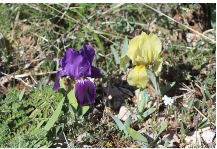
Iris lutescens Lam. (Iridaceae) is a widespread species in the Northern part of the Mediterranean basin. The species has been described in Spain, South of France and Italy under various botanical names, including I. chamaeiris Bertol., I. italica Parl., I. neglecta Parl., I. olbiensis Hénon, I. subbiflora Brot. and I. virescens Redouté (Crespo 2014, Tison et al. 2014, Colasante & Maury 2014). The species is rhizomatous and individuals show sword-like green leaves that are persistent all over the year. During the flowering period (March-May), individuals produce flowering stems bearing a unique showy and coloured flower (Figure 1). Various colour morph have been described (white, yellow-pale, pure yellow, purple, blue-purple...) but most of these phenotypes are rare in natural populations. Only the yellow and purple colour morphs are constant through the distribution range of the species. The species is self-incompatible and nectar-less, thus its pollination depends on naive insects emerging early in Spring (Imbert et al. 2014a).

Sampling design

Population locations were found using data from herbaria (VAL Valencia, Spain and MPU Montpellier, France), botanical publications (e.g. Mateos Sanz et al. 2003) and personal communications (P. Aymerich, A. Bonet, R. Calatyud, R. Leras J. Pedrol L. Serra, M. Talavera and S. Talavera, for Spain, and L. Minuto, G. Pellegrino for Italy) During four consecutive years (2011-2015), 80 populations have been surveyed during the flowering period (March-May). The sampling covers the distribution area of the species (Figure 2). For each population, the GPS coordinates and elevation were recorded. In each population, non-linear transects were defined using natural paths and the number of flowering stems was counted. Each flower was visually categorized either as yellow or as purple. The length and the number of the transects depended on the population size. Some populations are very small and just contain less than ten patches on 25 m long (e.g. Garraf population in Spain), while some populations contain thousand of individuals distributed over more than 5 hectares (e.g. Vedas in France). These countings were used to estimate the population size (total number of flowering stems without information about the number of genets), the frequency of the yellow morph (FYM) and of the purple morph (1 – FYM).

Some populations (n=31) have been visited at least in two different years, in particular populations close to Montpellier, to confirm the constancy of the frequency of the

(7)

yellow morph (see Appendix 1). When several FYM estimations were available for a population, the estimation with the highest number of flowering plants was used in the data analyses (in particular data collected in 2013, a favourable year for Iris blooming).

Abiotic data

Bioclimatic variables were extracted from the WorldClim version 2.0 database (Fick & Hijmans 2017) using a grid of 1 km². Data are extrapolated from 1970-2000 observations. From the 19 bioclimatic variables available, six variables describing temperature (annual mean temperature, mean diurnal range, temperature seasonality, maximal temperature of the warmest month, minimal temperature of the coldest month, temperature annual range) and five variables for precipitation (annual precipitation, precipitation of the wettest month, precipitation of the driest month, precipitation seasonality, precipitation of the driest quarter) were retained (Walisch et al. 2015). Because of correlations among these climatic variables, a principal component analysis was used to reduce the number of variables (see Appendix 2). The first three axes of the PCA explained 89.6 % of the total variance (40.9, 35.6 and 13.0 % respectively for PC1, PC2 and PC3). These three principal components were retained using the Horn’s parallel analysis performed using the R package paran (version 1.5.2).

UV irradiance data with 5 km spatial resolution are derived from the HelioClim-3 database of solar irradiance obtained from satellite data (Rigollier et al. 2004). Albedo of the ground was fixed at 0.2. Raw data were recorded from the 1 February 2004 to the 31 October 2015. Finally, aridity data have been extracted from the Global Aridity Index database (1 km² resolution) for the 1970-2000 period (Trabucco and Zomer 2018). Aridity index is positively correlated to precipitation and low values are associated to high water stress.

Data analyses

First, paired t-tests were applied using FYM values arc-sin transformed to test whether FYM varied over years for the 31 populations visited several times.

The variable to be explained was the number of yellow flowers, considered as a binomial variable, compared to the number of purple flowers per population. For each population, the explanatory variables were the population size, elevation, coordinates on the first three axes of the PCA for the bioclimatic data, UV irradiance and aridity

(8)

index. We first performed a generalized linear model for binomial variable including all the explanatory variables. Both residuals from the full model and from the null model showed a significant spatial autocorrelation (Moran’s index = 0.10, p<0.003 and index=0.34, p<0.0001, respectively for the full model and the null model). Thus, in order to consider the spatial autocorrelation, all analyses were performed using the spaMM package (version 3.0.0, Rousset & Ferdy 2014) under R version 3.6.2, including latitude and longitude coordinates as spatial information. To test for an effect of population size, and thus random process on FYM, a specific linear model was implemented with a random effect associated to population size (see Appendix 4).

Results

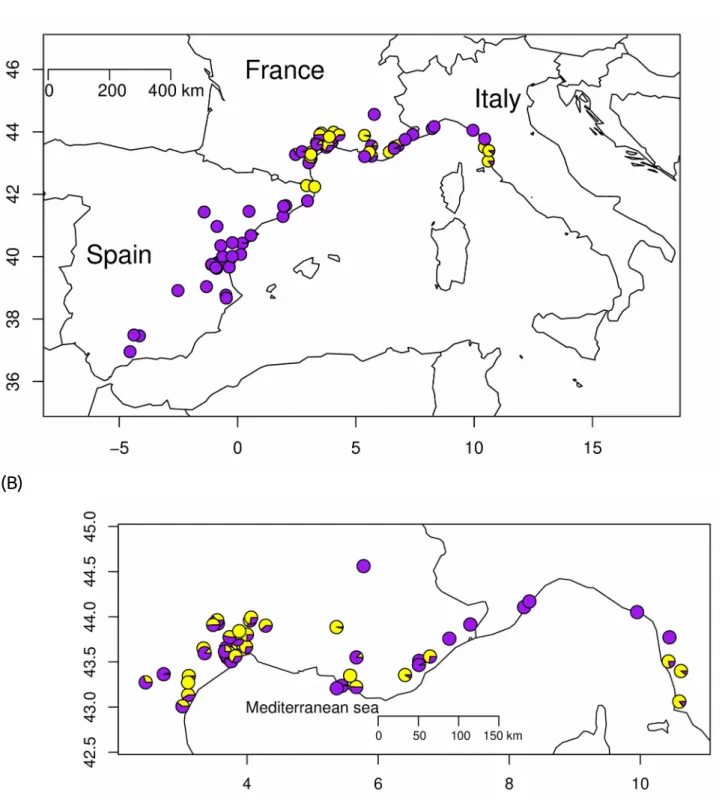
For the 31 populations that have been visited at least twice, no significant variation over years could be detected (paired t-tests, p>0.64). The mean frequency of the yellow morph was 0.31, but a huge variation for FYM was observed (SD 0.36, coefficient of variation 116%). 38 populations were monomorphic, either with the purple phenotype (n=33) or the yellow one (n=5). Purple dominant populations (FYM<0.25, n=45) were more frequent than yellow dominant populations (FYM>0.75, n=12). The frequency of yellow morph showed a geographical structure , since populations in Spain are mostly purple monomorphic (Figure 2a), with the exception of two populations close to the Pyrenees which were yellow monomorphic (Figure 2a). However, no structure is apparent in France and Italy (Figures 2b and c).

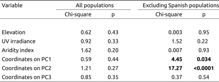
The generalized linear model including a random effect associated to population size had a likelihood lower than the model excluding this random effect (296.82 versus -289.66, see Appendix 4), thus this random effect was not conserved in the following analyses. Using the generalized linear model taking into account the spatial autocorrelation, none of the explanatory variables was significant (Table 1).

To go further, analyses were performed excluding populations sampled in Spain. Only 50 populations were thus considered in this new dataset. The pattern of spatial autocorrelation for FYM was less obvious (Figures 2b &c), and Moran’s indexes decreased to 0.07 using the residuals from the null model (p<0.04) and to 0.06 using the residuals from the full model (p=0.067). Generalized linear models indicated a significant effect for the first and the second principal components of the PCA performed on bioclimatic variables (Table 1). Consistently, the estimated coefficients for the Matérn function, representing the spatial autocorrelation, differed between the null model (ν=0.31, ρ=

(9)

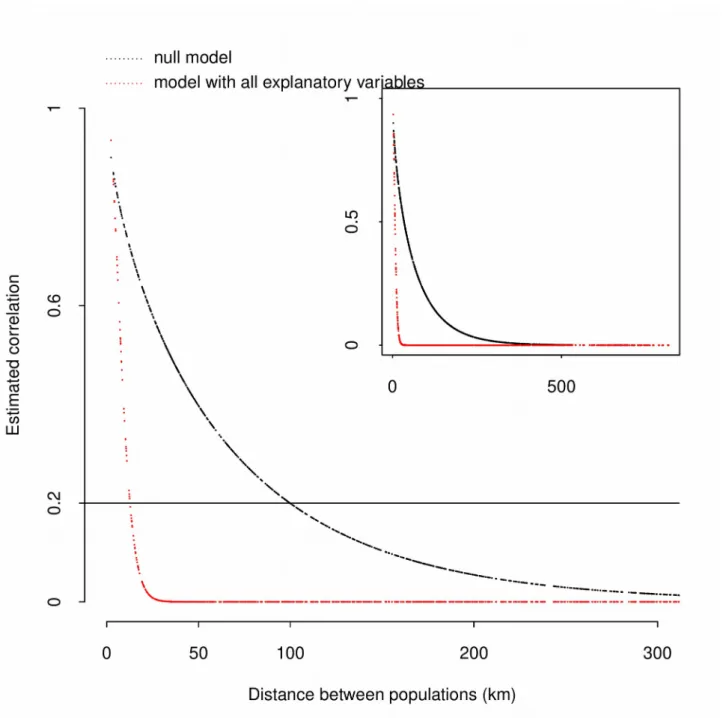
1.18) and the model including the two significant covariates (ν=4.40, ρ= 41.36). Spatial correlation for FYM decreased very rapidly and populations more than 50 km away (263 comparisons) had a correlation below 0.6 (Figure 3). Considering the null model, the correlation was below 0.2 for populations distant from 100 km (420 pairs out of 1225), while the correlation was almost null considering the model with the two significant covariates (Figure 3).

The first component of the PCA is negatively correlated to annual temperature (r=-0.86) and minimal temperature of the coldest month (r=-0.94) and positively correlated to variables representing precipitations, in particular to precipitations of the driest quarter of the year (r=0.93, Appendix 3, Table A3). The second component of the PCA is positively correlated to variables representing temperature ranges, in particular the mean diurnal range (r=0.71) and the maximal temperature (r=0.66, Table A3). The coordinates on PC1 and PC2 were thus replaced by the observed values of two bioclimatic variables, one representing precipitation and correlated to PC1 (precipitations of the driest quarter of the year, r=0.93 with PC1), and one for temperature and correlated to PC2 (annual range of temperature, r=0.66 with PC2). Both bioclimatic variables had a significant effect on FYM variation : Χ2_{= 10.58, p<0.002,} for annual range of temperature and Χ2_{= 10.46, p<0.002 for the precipitations of the} driest quarter.

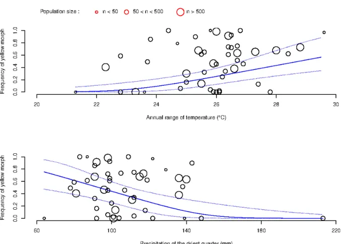
The frequency of the yellow morph significantly increased with the annual range of temperature (Figure 4a). Indeed, yellow dominant populations were only found in localities with large difference between the warmest month of the year and the coldest month, while purple dominant populations have be found in all situations (Figure 4a). Such differentiation was also observed in relation to precipitations of the driest quarter (Figure 4b), and yellow dominant populations occurred in localities with low precipitations, while purple dominant populations were found over the complete range of precipitations (Figure 4b). Despite significant relationships, it should be noticed that the correlation between FYM and annual range of temperature was very low (r=0.32, p=0.02), while the correlation with the precipitation variable was not significant (r=-0.12, p=0.39). A linear model including both variables only explained 28.5% of the variance observed for FYM.

(10)

Discussion

Flower colour polymorphism has been described in several plants (Rausher 2008, Narbona et al. 2018, Dormont et al. 2019), but few studies have reported the spatial distribution of the polymorphism over the distribution area of a single species. In deceptive plant species, negative frequency-dependent selection due to pollinator behaviour should produce a stable polymorphism within populations and no monomorphic population should be observed. In the deceptive orchid Dactylorhiza sambucina, a well-studied species with FCP, the mean frequency of the yellow morph is 0.69 with a low variation among populations (SD 0.03) in the South of France (Cévennes), (Gigord et al. 2001), but yellow monomorphic populations have been observed in Germany (Kropf & Renner 2008). In Sweden, populations are purple dominant with the frequency of yellow morph ranging from 0.07 to 0.65 (Jersáková et al. 2006). Finally, Smithson et al. (2007) also reported a large range for morph frequencies, with purple and yellow dominant populations, over the distribution area of the species. In Iris lutescens, the purple phenotype appeared to be more frequent than the yellow one, in particular in Spain, as reported by Crespo (2014), but also in Italy and in the South of France. While yellow monomorphic populations are less frequent, yellow dominant populations have also been observed across the distribution area of the species. These observations, combined with other studies on the pollination biology of the species (Imbert et al. 2014a, Imbert et al. 2014b, Souto-Vilarós et al. 2018) are not consistent with the expectations from negative-frequency dependent selection.

While investigations on plant physiology suggest pigment concentrations influence plant resistance to various abiotic stresses (Steyn et al. 2002), few studies have reported on the effects of abiotic factors, such as temperature, rainfall and solar radiation, on proportions of flower colour morphs. In species where FCP is influenced by bioclimatic variables, spatial autocorrelation and clinal variations are expected (Arista et al. 2013, Carlson & Holsinger 2015, Vaidya et al. 2018). The populations of Iris lutescens showed a low spatial autocorrelation in morph frequencies, except in Spain, and clearly no clinal variation could be observed. Actually, observations of spatial autocorrelation also depend on pigment expressions in vegetative tissues. In Iris lutescens, the concentrations of both anthocyanins and flavonoids, responsible for the purple and the yellow colouration respectively, are not different between morphs in vegetative parts (Wang et al. 2013). The differentiation in flower pigmentation often results from gene mutation leading to loss of function, and because of the various role of anthocyanins

(11)

and flavonoids in plant physiology, lost of function for structural genes is supposed to be highly counter-selected (Rausher 2008) As a consequence, anthocyanin production should be quite similar in vegetative tissues, as observed in I. lutescens (Wang et al. 2013) and only be modulated during flower bud production due to mutation in regulatory genes.

Other studies have reported that the difference between morphs in pigments concentration in vegetative tissues are induced by stress, and only visible in stressing conditions (Warren & Mackenzie 2001 , Strauss et al. 2004, Sobel et al. 2019). Therefore, flower colour can be viewed as a phenotype related to the individual ability to resist to abiotic stress, i.e. plasticity to some stressing conditions. In such situations, pigmentation should show a geographic structure (Dalrymple et al. 2020, Peach et al. 2020). Following studies reporting that anthocyanins contribute to water stress resistance (Warren & Mackenzie 2001, Schemske & Bierzychudek 2007, Arista et al. 2013, Sobel et al. 2019), the purple morph of Iris lutescens should be dominant in arid habitats. Considering only the Spanish localities where populations of Iris lutescens have been found, both the precipitations of the driest quarter (mean = 77.53 mm SD 29.45) and annual range of temperature (mean = 28.65°C SD 3.03) showed extreme values in comparison to values observed for South of France (precipitation mean = 105.97 mm SD 24.30, range of temperature mean = 25.94°C, SD 1.59) and for Italy (precipitation mean = 120.43 mm SD 24.96, range of temperature mean = 24.22°C, SD 1.18). Therefore, the observation of monomorphic purple populations in Spain is consistent with this hypothesis since aridity is greater in Spain than in the South of France and Italy. However, the absence of clinal variation between the purple and the yellow morph is not consistent with this hypothesis. Furthermore, purple dominant populations were observed through all the range of bioclimatic factors, even in Italy where water stress is low.

Producing pigmented flowers also influences water balance in floral tissues, since darker pigmentation increases light absorbance and tissues temperature, and finally evapotranspiration (Roddy 2019). Dark flowers are thus more costly to produce, in particular in arid habitats and in latitudes with high UV irradiance. Flower colour also influences anther temperature, and thus pollen quality (Mu et al. 2017) or pollen resistance to heat (Koski & Galloway 2018). It is likely that all these factors also contribute to the local frequency of the purple and yellow morphs, but clearly the results from this study showed that the relationships between the considered abiotic factors and morph frequencies were very low.

(12)

Since flower colour is genetically determined, classical factors affecting allele frequencies, such as migration and drift (Epperson & Clegg 1986) and founder events (Keasar et al. 2016) have also to be considered. The karyotypes of individuals of Iris lutescens from Italian populations suggest the species is closed to Iris attica, another species with FCP occurring in Eastern Europe (Greece, Balkans, Turkey…), a phylogenetic proximity confirmed by molecular approaches (Wilson 2017). Therefore, the species probably originates from the East of Europe and populations in Spain are likely to be the most recent ones. During the colonization from East to West, i.e. from Italy to Spain, repeated founder events could have contributed to the loss of the yellow phenotypes. Wang et al. (2016) have reported that Spanish populations and monomorphic populations from France have low genetic diversity which could result from such founder events. It can also be hypothesized that Spanish populations originated from a refugia in Southern Spain, while French and Italian populations originated from other refugia, the Pyrenees being a barrier between the two fronts of expansion (Médail & Diadema 2009). While floral traits have been repeatedly studied in relation to pollinators, historical contingencies have also to be considered to understand the spatial distribution of phenotypes, and a phylogeography of the species has to be built.

(13)

Acknowledgements

I thank P. Aymerich, A. Bonet, R. Calatyud, R. Leras, L. Minuto, J. Pedrol, G. Pellegrino, L. Serra, M. Talavera and S. Talavera for helping in finding localities. I also thank M. Arista, P. Ortiz, M. Talavera and H. Wang for fruitful discussions about flower colour polymorphism, and F. Rousset for his help with data analyses. Two anonymous reviewers made some suggestions that contributed to clarify this manuscript. Finally, I am particularly indebted to Béatrice Hervouet for supporting me during field works. The first draft of this manuscript was written during a sabbatical period in the department of Botany of the University of Sevilla.

(14)

Literature cited

Arista M, Talavera M, Berjano R, Ortiz PL. 2013. Abiotic factors may explain the geographical distribution of flower colour morphs and the maintenance of colour polymorphism in the scarlet pimpernel. J Ecol. 101(6):1613–1622.

Carlson JE, Holsinger KE. 2015. Extrapolating from local ecological processes to genus-wide patterns in colour polymorphism in South African Protea. Proc R Soc B Biol Sci. 282(1806):20150583.

Caruso CM, Eisen KE, Martin RA, Sletvold N. 2019. A meta-analysis of the agents of selection on floral traits: meta-analysis of selection on floral traits. Evolution. 73(1):4– 14.

Colasante MA, Maury AE 2014. Iridaceae present in Italy, Edited by Sapienza Universita di Roma, 416 pages.

Crespo M.B 2014. Iris L. in S. Talavera, C. Andrés, M. Arista, M.P. Fernández Piedra, E. Rico, M.B. Crespo, A. Quintanar, A. Herrero & C. Aedo,. (eds.). Flora iberica XX: 412-415. Real Jardín Botánico, CSIC, Madrid.

Dalrymple RL, Kemp DJ, Flores Moreno H, Laffan SW, White TE, Hemmings FA, Moles AT.‐Moreno H, Laffan SW, White TE, Hemmings FA, Moles AT. 2020. Macroecological patterns in flower colour are shaped by both biotic and abiotic factors. New Phytol. : doi: 10.1111/nph.16737

Dormont L, Delle-Vedove R, Bessière J-M, Hossaert-Mc Key M, Schatz B. 2010. Rare white-flowered morphs increase the reproductive success of common purple morphs in a food-deceptive orchid. New Phytologist. 185(1):300–310.

Dormont L, Joffard N, Schatz B. 2019. Intraspecific variation in floral color and odor in Orchids. Int J Plant Sci. 180(9):1036–1058.

Epperson BK, Clegg MT. 1986. Spatial-autocorrelation analysis of flower color polymorphisms within substructured populations of morning glory (Ipomoea purpurea). Am Nat. 128(6):840–858.

Fick SE, Hijmans RJ. 2017. WorldClim 2: new 1-km spatial resolution climate surfaces for global land areas: new climate surfaces for global land areas. Int J Climatol. 37(12):4302–4315.

Gigord LDB, Macnair MR, Smithson A. 2001. Negative frequency-dependent selection maintains a dramatic flower color polymorphism in the rewardless orchid Dactylorhiza sambucina (L.) Soo. Proc Natl Acad Sci. 98(11):6253–6255.

Groiß AM, Braun A, Greimler J, Kropf M. 2017. Pollen tracking in the food-deceptive orchid Dactylorhiza sambucina showed no predominant switching behaviour of

(15)

pollinators between flower colour morphs. Flora. 232:194–199.

Imbert E, Wang H, Anderson B, Hervouet B, Talavera M, Schatz B. 2014a. Reproductive biology and colour polymorphism in the food-deceptive Iris lutescens (Iridaceae). Acta Bot Gallica. 161(2):117–127.

Imbert E, Wang H, Conchou L, Vincent H, Talavera M, Schatz B. 2014b. Positive effect of the yellow morph on female reproductive success in the flower colour polymorphic Iris lutescens (Iridaceae), a deceptive species. J Evol Biol. 27(9):1965–1974.

Jersáková J, Kindlmann P, Renner SS. 2006. Is the colour dimorphism in Dactylorhiza sambucina maintained by differential seed viability instead of frequency-dependent selection? Folia Geobot. 41(1):61–76.

Keasar T, Gerchman Y, Lev-Yadun S. 2016. A seven-year study of flower-color polymorphism in a Mediterranean annual plant. Basic Appl Ecol. 17(8):741–750.

Koski MH, Galloway LF. 2018. Geographic variation in pollen color is associated with temperature stress. New Phytol. 218(1):370–379.

Kropf M, Renner SS. 2008. Pollinator-mediated selfing in two deceptive orchids and a review of pollinium tracking studies addressing geitonogamy. Oecologia. 155(3):497– 508.

Mateo Sanz G, Torres Gómez C., Fabado Alós J. 2003. Adiciones al catálogo de la flora de las comarcas valencianas de los Serranos y Ademuz, II. Flora Montiberica 25: 10-23. Médail F., Diadema K 2009. Glacial refugia influence plant diversity patterns in the

Mediterranean Basin. J Biog. 36 : 1333-1345.Mu J, Yang Y, Luo Y, Su R, Niklas KJ. 2017. Pollinator preference and pollen viability mediated by flower color synergistically determine seed set in an Alpine annual herb. Ecol Evol. 7(9):2947–2955.

Narbona E, Wang H, Ortiz PL, Arista M, Imbert E. 2018. Flower colour polymorphism in the Mediterranean Basin: occurrence, maintenance and implications for speciation. Plant Biol. 20:8–20.

Ojeda F, Midgley J, Pauw A, Lavola A, Casimiro-Soriguer R, Hattas D, Segarra-Moragues JG, Julkunen-Tiitto R. 2019. Flower colour divergence is associated with post-fire regeneration dimorphism in the fynbos heath Erica coccinea subsp. coccinea (Ericaceae). Evol Ecol. 33(3):345–367.

Peach K, Liu JW, Mazer SJ. 2020. Climate Predicts UV Floral Pattern Size, Anthocyanin Concentration, and Pollen Performance in Clarkia unguiculata. Front Plant Sci. 11: article847.

Pellegrino G, Bellusci F, Musacchio A. 2005. Evidence of post-pollination barriers among three colour morphs of the deceptive orchid Dactylorhiza sambucina (L.) Soó. Sex Plant

(16)

Reprod. 18(4):179–185.

Rausher MD. 2008. Evolutionary Transitions in Floral Color. Int J Plant Sci. 169(1):7–21. Rigollier C, Lefèvre M, Wald L. 2004. The method Heliosat-2 for deriving shortwave solar

radiation from satellite images. Sol Energy. 77(2):159–169.

Roddy AB. 2019. Energy balance implications of floral traits involved in pollinator attraction and water balance. Int J Plant Sci. 180(9):944–953.

Rousset F, Ferdy J-B. 2014. Testing environmental and genetic effects in the presence of spatial autocorrelation. Ecography. 37(8):781–790.

Sapir Y, Brunet J, Byers DL, Imbert E, Schönenberger J, Staedler Y. 2019. Floral evolution: breeding systems, pollinators, and beyond. Int J Plant Sci. 180(9):929–933.

Sapir Y, Ghara M. 2017. The (relative) importance of pollinator-mediated selection for evolution of flowers. Am J Bot. 104(12):1787–1789.

Schemske DW, Bierzychudek P. 2007. Spatial differentiation for flower color in the desert annual Linanthus parryae: was Wright right? Evolution. 61(11):2528–2543.

Smithson A, Juillet N, Macnair MR, Gigord LDB. 2007. Do rewardless orchids show a positive relationship between phenotypic diversity and reproductive success? Ecology. 88(2):434–442.

Sobel JM, Stankowski S, Streisfeld MA. 2019. Variation in ecophysiological traits might contribute to ecogeographic isolation and divergence between parapatric ecotypes of Mimulus aurantiacus. J Evol Biol. 32(6):604–618.

Sobel JM, Streisfeld MA. 2015. Strong premating reproductive isolation drives incipient speciation in Mimulus aurantiacus. Evolution. 69(2):447–461.

Sobral M, Veiga T, Domínguez P, Guitián JA, Guitián P, Guitián JM. 2015. Selective pressures explain differences in flower color among Gentiana lutea populations. PLOS ONE. 10(7):e0132522.

Souto-Vilarós D, Vuleta A, Jovanović SM, Budečević S, Wang H, Sapir Y, Imbert E. 2018. Are pollinators the agents of selection on flower colour and size in irises? Oikos. 127(6):834–846.

Steyn WJ, Wand SJE, Holcroft DM, Jacobs G. 2002. Anthocyanins in vegetative tissues: a proposed unified function in photoprotection. New Phytol. 155(3):349–361.

Strauss SY, Irwin RE, Lambrix VM. 2004. Optimal defence theory and flower petal colour predict variation in the secondary chemistry of wild radish: Patterns of plant variation in defence. J Ecol. 92(1):132–141.

Tanaka Y, Sasaki N, Ohmiya A. 2008. Biosynthesis of plant pigments: anthocyanins, betalains and carotenoids. Plant J. 54(4):733–749.

(17)

Tang X-X, Huang S-Q. 2010. Fluctuating selection by water level on gynoecium colour polymorphism in an aquatic plant. Ann Bot. 106(5):843–848.

Tison J.M., Jauzein P., Michaud H. (2014). Flore de la France méditerranéenne continentale. Edited by Naturalia Publications, 2080 pages. Page 265.

Trabucco, A., and Zomer, R.J. (2018). Global Aridity Index and Potential Evapo-Transpiration (ET0) Climate Database v2. CGIAR Consortium for Spatial Information (CGIAR-CSI). Published online, available from the CGIAR-CSI GeoPortal at https://cgiarcsi.community

Vaidya P, McDurmon A, Mattoon E, Keefe M, Carley L, Lee C-R, Bingham R, Anderson JT. 2018. Ecological causes and consequences of flower color polymorphism in a self-pollinating plant ( Boechera stricta ). New Phytol.

Veiga T, Guitián Javier, Guitián P, Guitián José, Munilla I, Sobral M. 2016. Flower colour variation in the montane plant Gentiana lutea L. (Gentianaceae) is unrelated to abiotic factors. Plant Ecol Divers. 9(1):105–112.

Walisch TJ, Colling G, Bodenseh M, Matthies D. 2015. Divergent selection along climatic gradients in a rare central European endemic species, Saxifraga sponhemica. Ann Bot. 115(7):1177–1190.

Wang H, Conchou L, Bessière J-M, Cazals G, Schatz B, Imbert E. 2013. Flower color polymorphism in Iris lutescens (Iridaceae): Biochemical analyses in light of plant–insect interactions. Phytochemistry. 94:123–134.

Wang H, Talavera M, Min Y, Flaven E, Imbert E. 2016. Neutral processes contribute to patterns of spatial variation for flower colour in the Mediterranean Iris lutescens (Iridaceae). Ann Bot. 117(6):995–1007.

Warren J, Mackenzie S. 2001. Why are all colour combinations not equally represented as flower-colour polymorphisms? New Phytol. 151(1):237–241.

Wilson CA. 2017. Sectional relationships in the Eurasian bearded Iris (subgen. Iris ) based on phylogenetic analyses of sequence data. Syst Bot. 42(3):392–401.

(18)

Table 1 : Summary of the likelihood-ratio test performed for each explanatory variable to explain the frequency of the yellow morph (treated as a binomial variable, see text for details). GLM have been performed using the spaMM package. Analyses have first been performed using the entire dataset (n=80 populations), and next excluding the Spanish populations (n=50 populations). All variables are covariates and df=1.

Variable All populations Excluding Spanish populations

Chi-square p Chi-square p Elevation 0.62 0.43 0.003 0.95 UV irradiance 0.92 0.33 1.52 0.22 Aridity index 1.62 0.20 0.007 0.93 Coordinates on PC1 0.59 0.44 4.45 0.034 Coordinates on PC2 1.21 0.27 17.27 <0.0001 Coordinates on PC3 0.85 0.35 0.37 0.54

(19)

Figure 1 Purple- and yellow-flowered individuals of Iris lutescens. Picture was taken by B. Hervouet, Causse de Blandas, Languedoc-Roussillon region, France.

(20)

Figure 2: Distribution of the sampled populations. The three maps differ in the scale and (A) represents the entire dataset (n=80 populations), (B) dataset excluding populations from Spain (n=50), and (C) populations sampled around Montpellier. The morph frequencies (yellow/purple) for each sampled population are shown as a pie chart.

(A)

(B)

(21)

(22)

Figure 3 : Spatial autocorrelation for the frequency of the yellow morph for all the sampled populations but the Spanish ones. Autocorrelation has been estimated using the Matérn function fitted in the generalized linear model including the two significant covariates (coordinates on PC1 and PC2, see Table 1) and using a null model (see text for details, and Appendix 4).

(23)

Figure 4 : Frequency of the yellow morph according to the annual range of temperature (upper panel) and precipitations of the driest quarter (lower panel) for the populations sampled in France and Italy (n=50). The size of each point depends on population size. The solid line represents the frequency of yellow morph as fitted in the generalizaed linear model including the two significant variables. Dotted lines represent the 95 % confidence intervals.

(24)

Appendix 1 : data table – Libreoffice format Two datasheets :

data : locality name (and country), GPS coordinates (WGS84 format), elevation (in meters), and number of yellow flowers and of purple flowers, and the values of the abiotic variables used in this paper. Aridity index values have been multiplied by a factor of 10,000.

Repetition : frequecy of yellow morph estimated for some populations that have been visited at least twice between 2011 and 2015. Results from paired t-tests are also given.

(25)

Appendix 2 : Summary of analyses for bioclimatic data using the entire dataset

Using GPS coordinates of each population, bioclimatic data have been extracted from the Worldclim database version 2.0. Six variables describing temperature and five for precipitation were retained :

Temperature

BIO1 = Annual Mean Temperature

BIO2 = Mean Diurnal Range (Mean of monthly (max temp - min temp)) BIO4 = Temperature Seasonality (standard deviation *100)

BIO5 = Max Temperature of Warmest Month BIO6 = Min Temperature of Coldest Month BIO7 = Temperature Annual Range (BIO5-BIO6) Precipitation

BIO12 = Annual Precipitation

BIO13 = Precipitation of Wettest Month BIO14 = Precipitation of Driest Month

BIO15 = Precipitation Seasonality (Coefficient of Variation) BIO17 = Precipitation of Driest Quarter

PCA was performed using the FactoMineR package and Horn’s parallel analysis for component retention (paran package). For results of the Horn’parallel analysis, see Appendix 4. The first three components were retained.

The first three axes of the PCA explained 89.6 % of the total variance : Eigenvalues

Dim.1 Dim.2 Dim.3 Dim.4 Variance 4.507 3.919 1.430 0.793 % of var. 40.976 35.627 13.003 7.210 Cumulative % of var. 40.976 76.603 89.607 96.817

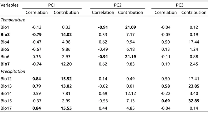
The first principal component is positively correlated with precipitation variables (in particular Bio12, Bio13 and Bio17) and negatively correlated with temperature range (Bio2 and Bio7), and thus represents the continentality of the station. The second PC clearly reflects the temperature (Bio1 and Bio6) while the third PC is correlated with seasonality (Bio13 and Bio15).

(26)

Table A2 : Correlations and contributions of bioclimatic variables for the first three principal components.

Variables PC1 PC2 PC3

Correlation Contribution Correlation Contribution Correlation Contribution Temperature Bio1 -0.12 0.32 -0.91 21.09 -0.04 0.12 Bio2 -0.79 14.02 0.53 7.17 -0.05 0.19 Bio4 -0.47 4.98 0.62 9.94 0.50 17.44 Bio5 -0.67 9.86 -0.49 6.18 0.13 1.24 Bio6 0.36 2.93 -0.91 21.19 -0.11 0.88 Bio7 -0.74 12.20 0.62 9.83 0.19 2.45 Precipitation Bio12 0.84 15.52 0.14 0.49 0.50 17.41 Bio13 0.79 13.82 -0.02 0.01 0.58 23.85 Bio14 0.59 7.81 0.69 12.12 -0.22 3.40 Bio15 -0.37 2.99 -0.53 7.13 0.69 32.89 Bio17 0.84 15.55 0.44 4.85 -0.04 0.14

(27)

Appendix 3 : Summary of analyses for bioclimatic data excluding Spanish populations For results of the Horn’parallel analysis, see Appendix 4. The first three components were retained. The 3 first axes of the PCA explained 91.38 % of the total variance :

Eigenvalues

Dim.1 Dim.2 Dim.3 Dim.4

Variance 6.279 2.080 1.719 0.567

% of var. 57.086 18.906 15.627 5.152

Cumulative % of var. 57.086 75.993 91.620 96.737

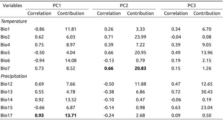
PC2 is negatively correlated with total precipitation (Bio12) and positively correlated with variables representing temperature ranges (Bio2, Bio5 and and Bio7).

(28)

Table A3 : Correlations and contributions of bioclimatic variables for the first three principal components, excluding localities from Spain.

Variables PC1 PC2 PC3

Correlation Contribution Correlation Contribution Correlation Contribution Temperature Bio1 -0.86 11.81 0.26 3.33 0.34 6.70 Bio2 0.62 6.03 0.71 23.99 -0.04 0.08 Bio4 0.75 8.97 0.39 7.22 0.39 9.05 Bio5 -0.50 4.04 0.66 20.95 0.49 13.96 Bio6 -0.94 14.08 -0.13 0.79 0.19 2.15 Bio7 0.73 8.52 0.66 20.83 0.15 1.26 Precipitation Bio12 0.69 7.66 -0.50 11.88 0.47 12.65 Bio13 0.55 4.78 -0.38 6.86 0.72 30.43 Bio14 0.92 13.52 -0.10 0.47 -0.06 0.19 Bio15 -0.66 6.87 -0.14 0.98 0.63 23.04 Bio17 0.93 13.71 -0.24 2.68 0.09 0.50

Appendix 4 : PDF output of the R script.

(29)

Data analyses for MS_XXXX

Eric Imbert June 2020 rm(list=ls()) setwd("~/Recherches/iris/lutescens/abiotic") library(spaMM)

## Registered S3 methods overwritten by 'registry':

## method from

## print.registry_field proxy ## print.registry_entry proxy

## spaMM (Rousset & Ferdy, 2014, version 3.2.0) is loaded. ## Type 'help(spaMM)' for a short introduction,

## 'news(package='spaMM')' for news,

## and 'citation(spaMM)' for proper citation.

library(FactoMineR)

library(car)

## Loading required package: carData

library(maps)

library(plotrix)

library(paran)

## Loading required package: MASS

#Import data => use the data sheet "census" from the Libreoffice file

donnees=read.csv('abiotic_data.csv',header=T, dec='.')

donnees$popsize=donnees$nbyellow+donnees$nbpurple

donnees$FYM=donnees$nbyellow/donnees$popsize

Step 1 : PCA for the abiotic variables Following Walisch et al 2015, just keep : Temperature : bio1, bio2, bio4,bio5, bio6, bio7 Rainfall : bio12, bio13, bio14, bio15, bio17

Climate variables Temperature BIO1 = Annual Mean Temperature BIO2 = Mean Diurnal Range (Mean of monthly (max temp - min temp)) BIO4 = Temperature Seasonality (standard deviation *100) BIO5 = Max Temperature of Warmest Month BIO6 = Min Temperature of Coldest Month BIO7 = Temperature Annual Range (BIO5-BIO6) Precipitation BIO12 = Annual Precipitation BIO13 = Precipitation of Wettest Month BIO14 = Precipitation of Driest Month BIO15 = Precipitation Seasonality (Coefficient of Variation) BIO17 = Precipitation of Driest Quarter

attach(donnees)

val=cbind(bio1,bio12,bio13,bio14, bio15,bio17,bio2,bio4,bio5,bio6,bio7)

multi_ana=PCA(val, scale.unit=T, graph=FALSE)

paran(val, iterations=5000, centile=95)

##

## Using eigendecomposition of correlation matrix.

## Computing: 10% 20% 30% 40% 50% 60% 70% 80% 90% 100% ##

##

## Results of Horn's Parallel Analysis for component retention ## 5000 iterations, using the 95 centile estimate

##

## ---## Component Adjusted Unadjusted Estimated ## Eigenvalue Eigenvalue Bias

(30)

## ---## 1 3.675256 4.507412 0.832155 ## 2 3.346847 3.918947 0.572099 ## 3 1.031152 1.430383 0.399231 ## ---##

## Adjusted eigenvalues > 1 indicate dimensions to retain. ## (3 components retained)

detach(donnees)

donnees$pc1=multi_ana$ind$coord[,1]

library(DHARMa)

## Registered S3 methods overwritten by 'lme4':

## method from

## cooks.distance.influence.merMod car

## influence.merMod car

## dfbeta.influence.merMod car ## dfbetas.influence.merMod car

## This is DHARMa 0.3.0. For overview type '?DHARMa'. For recent changes, type news(package = 'DHARMa') Note: Syntax of plotResiduals has changed in 0.3.0, see ?plotResiduals for details fullglm=glm(cbind(nbyellow,nbpurple) ~

popsize + elevation + UV + aridity + pc1 + pc2 + pc3,

family=binomial, data=donnees) nullglm=glm(cbind(nbyellow,nbpurple) ~ 1,

family=binomial, data=donnees) sims <- simulateResiduals(fullglm, n=1000)

testSpatialAutocorrelation(sims, x = donnees$lon, y = donnees$lat, plot = TRUE)

−5 0 5 10

38

40

42

44

DHARMa Moran's I test for spatial autocorrelation

x

y

##

## DHARMa Moran's I test for spatial autocorrelation 2

(31)

## ## data:

## observed = 0.100551, expected = -0.012658, sd = 0.036735, p-value = ## 0.002058

## alternative hypothesis: Spatial autocorrelation sims_null <- simulateResiduals(nullglm, n=1000)

testSpatialAutocorrelation(sims_null, x = donnees$lon, y = donnees$lat, plot = TRUE)

−5 0 5 10

38

40

42

44

x

y

##

## DHARMa Moran's I test for spatial autocorrelation ##

## data:

## observed = 0.345776, expected = -0.012658, sd = 0.036773, p-value < ## 2.2e-16

## alternative hypothesis: Spatial autocorrelation

Can FYM be explained by random process due to population size ?

The model includes a random factor associated to 1/sqrt(population size) Population size is standardized to avoid estimation of large values of variances

donnees$std_popsize=donnees$popsize/mean(donnees$popsize)

donnees$popvar=1/sqrt(donnees$std_popsize)

fit1=fitme(cbind(nbyellow,nbpurple) ~

elevation + UV + aridity + pc1 + pc2 + pc3 +

Matern(popvar-1|lat + lon),

data=donnees, family=binomial(), method="REML", control=list(max.iter=1000, max.iter.mean=500), init=list(lambda=NaN))

## Iterative algorithm converges slowly. See help('convergence') for suggestions. fit2=fitme(cbind(nbyellow,nbpurple) ~

Matern(1|lat + lon),

data=donnees, family=binomial(), method="REML", control=list(max.iter=1000, max.iter.mean=500),

(32)

init=list(lambda=NaN))

## Iterative algorithm converges slowly. See help('convergence') for suggestions.

#Marginal value of Likelihood for each model

fit1$APHLs$p_bv

## [1] -296.8298 fit2$APHLs$p_bv

## [1] -289.6606

Likelihood is maximal without the random effect of population size.

Ad-hoc procedure to check the maximum value of likelihood - this part of the script has been written with François Rousset - see various documents about spaMM for details.

oncherche=function(w) {

varfac=w+(1-w)*(donnees$std_popsize) #varfac=1 for w=1 and varfac=donnees$std_popsize for w=0

donnees$weisd=1/sqrt(varfac) # weisd=1 for w=1 and weisd=popvar for w=0

new_fit=fitme(cbind(nbyellow,nbpurple) ~

Matern(weisd-1|lat + lon),

data=donnees, family=binomial(), method="PQL", control=list(max.iter=1000, max.iter.mean=500), init=list(lambda=NaN))

Rel=new_fit$APHLs$p_bv

print(c(w=w,Rel=Rel))

#return(-Rel)

}

a=optimize(oncherche, interval=c(0,1))

a

=> so the maximal value is obtained with the model without popvar, which excludes contribution of population size to the observed pattern.

Global analyses

nullfit=fitme(cbind(nbyellow,nbpurple) ~ 1 +

Matern(1|lat + lon), data=donnees,

family=binomial(), method="ML",

control.HLfit=list(max.iter=1000, max.iter.mean=500)) fullfit=fitme(cbind(nbyellow,nbpurple) ~

Matern(1|lat + lon),

data=donnees, family=binomial(),method="ML",

control.HLfit=list(max.iter=1000, max.iter.mean=500))

LRT(fullfit,nullfit)

## chi2_LR df p_value ## p_v 8.568931 6 0.1993115

summary(fullfit)

## formula: cbind(nbyellow, nbpurple) ~ elevation + UV + aridity + pc1 + ## pc2 + pc3 + Matern(1 | lat + lon)

## Estimation of corrPars and lambda by Laplace ML approximation (p_v). ## Estimation of fixed effects by Laplace ML approximation (p_v). ## Estimation of lambda by 'outer' ML, maximizing p_v.

## Family: binomial ( link = logit )

## Fixed effects (beta) ---## Estimate Cond. SE t-value

(33)

## (Intercept) 63.760270 47.265823 1.349 ## elevation -0.009543 0.006306 -1.513 ## UV -0.001315 0.001277 -1.030 ## aridity -0.004258 0.002625 -1.622 ## pc1 2.198891 1.649735 1.333 ## pc2 1.495679 0.933498 1.602 ## pc3 1.672643 1.564778 1.069 ## Random effects ---## Family: gaussian ( link = identity )

## --- Correlation parameters:

## 1.nu 1.rho

## 0.8551812 5.4681193

## --- Variance parameters ('lambda'): ## lambda = var(u) for u ~ Gaussian;

## lat + lon : 30.05

## # of obs: 80; # of groups: lat + lon, 80

## Likelihood values

---## logLik

## p_v(h) (marginal L): -278.873

summary(nullfit)

## formula: cbind(nbyellow, nbpurple) ~ 1 + Matern(1 | lat + lon) ## Estimation of corrPars and lambda by Laplace ML approximation (p_v). ## Estimation of fixed effects by Laplace ML approximation (p_v). ## Estimation of lambda by 'outer' ML, maximizing p_v.

## (Intercept) -10.21 2.523 -4.048

## Random effects ---## Family: gaussian ( link = identity )

## 1.nu 1.rho

## 0.5259553 1.2285802

## lat + lon : 61.12

---## logLik

## p_v(h) (marginal L): -283.1574

No difference between the null model and the full model one by one => p-values in Table 1

test_elevation=fitme(cbind(nbyellow,nbpurple) ~

UV + aridity + pc1 + pc2 + pc3 +

control.HLfit=list(max.iter=1000, max.iter.mean=500)) test_UV=fitme(cbind(nbyellow,nbpurple) ~

elevation + aridity + pc1 + pc2 + pc3 +

control.HLfit=list(max.iter=1000, max.iter.mean=500)) test_aridity=fitme(cbind(nbyellow,nbpurple) ~

elevation + UV + pc1 + pc2 + pc3 +

## Iterative algorithm converges slowly. See help('convergence') for suggestions. 5

(34)

test_pc1=fitme(cbind(nbyellow,nbpurple) ~

elevation + UV + aridity + pc2 + pc3 +

## Iterative algorithm converges slowly. See help('convergence') for suggestions. test_pc2=fitme(cbind(nbyellow,nbpurple) ~

## Iterative algorithm converges slowly. See help('convergence') for suggestions. test_pc3=fitme(cbind(nbyellow,nbpurple) ~

## Iterative algorithm converges slowly. See help('convergence') for suggestions.

LRT(fullfit,test_elevation) ## chi2_LR df p_value ## p_v 0.6206077 1 0.4308215 LRT(fullfit,test_UV) ## chi2_LR df p_value ## p_v 0.9197677 1 0.337536 LRT(fullfit,test_aridity) ## chi2_LR df p_value ## p_v 1.626021 1 0.2022543 LRT(fullfit,test_pc1) ## chi2_LR df p_value ## p_v 0.5987665 1 0.4390491 LRT(fullfit,test_pc2) ## chi2_LR df p_value ## p_v 1.215451 1 0.2702553 LRT(fullfit,test_pc3) ## chi2_LR df p_value ## p_v 0.8511212 1 0.3562354 Figures 2

The same analyses but excluding populations from Spain notspain=subset(donnees, country!="spain")

attach(notspain)

val=cbind(bio1,bio12,bio13,bio14, bio15,bio17,bio2,bio4,bio5,bio6,bio7)

multi_ana=PCA(val, scale.unit=T, graph=FALSE)

paran(val, iterations=5000, centile=95)

##

## Using eigendecomposition of correlation matrix.

## Computing: 10% 20% 30% 40% 50% 60% 70% 80% 90% 100% ##

##

## Results of Horn's Parallel Analysis for component retention ## 5000 iterations, using the 95 centile estimate

(35)

##

## ---## Component Adjusted Unadjusted Estimated ## Eigenvalue Eigenvalue Bias

## ---## 1 5.203709 6.279497 1.075787 ## 2 1.345862 2.079679 0.733816 ## 3 1.210014 1.719011 0.508996 ## ---##

## Adjusted eigenvalues > 1 indicate dimensions to retain. ## (3 components retained)

detach(notspain)

notspain$pc1=multi_ana$ind$coord[,1]

library(DHARMa)

fullglm=glm(cbind(nbyellow,nbpurple) ~

popsize + elevation + UV + aridity + pc1 + pc2 + pc3,

family=binomial, data=notspain)

nullglm=glm(cbind(nbyellow,nbpurple) ~ 1, family=binomial, data=notspain)

sims <- simulateResiduals(fullglm, n=1000)

testSpatialAutocorrelation(sims, x = notspain$lon, y = notspain$lat, plot = TRUE)

4 6 8 10

43.0

43.5

44.0

44.5

x

y

##

## data:

## alternative hypothesis: Spatial autocorrelation

(36)

sims_null <- simulateResiduals(nullglm, n=1000)

testSpatialAutocorrelation(sims_null, x = notspain$lon, y = notspain$lat, plot = TRUE)

4 6 8 10

43.0

43.5

44.0

44.5

x

y

##

## data:

## alternative hypothesis: Spatial autocorrelation nullfit=fitme(cbind(nbyellow,nbpurple) ~ 1 +

Matern(1|lat + lon), data=notspain,

control.HLfit=list(max.iter=1000, max.iter.mean=500)) fullfit=fitme(cbind(nbyellow,nbpurple) ~

Matern(1|lat + lon), data=notspain, family=binomial(),

method="ML", control.HLfit=list(max.iter=1000, max.iter.mean=500))

LRT(fullfit,nullfit)

summary(fullfit)

## formula: cbind(nbyellow, nbpurple) ~ elevation + UV + aridity + pc1 + ## pc2 + pc3 + Matern(1 | lat + lon)

## Estimation of corrPars and lambda by Laplace ML approximation (p_v). ## Estimation of fixed effects by Laplace ML approximation (p_v). ## Estimation of lambda by 'outer' ML, maximizing p_v.

## Fixed effects (beta) ---## Estimate Cond. SE t-value ## (Intercept) -2.941e+01 2.729e+01 -1.07762

(37)

## elevation -3.369e-04 5.681e-03 -0.05931 ## UV 8.298e-04 7.474e-04 1.11017 ## aridity 1.199e-04 1.547e-03 0.07748 ## pc1 -2.257e-01 6.956e-01 -0.32454 ## pc2 1.505e+00 9.203e-01 1.63513 ## pc3 -3.063e-01 6.282e-01 -0.48762 ## Random effects ---## Family: gaussian ( link = identity )

## 1.nu 1.rho ## 13.92716 80.69473

## lat + lon : 9.886

---## logLik

## p_v(h) (marginal L): -240.2823

summary(nullfit)

## formula: cbind(nbyellow, nbpurple) ~ 1 + Matern(1 | lat + lon) ## Estimation of corrPars and lambda by Laplace ML approximation (p_v). ## Estimation of fixed effects by Laplace ML approximation (p_v). ## Estimation of lambda by 'outer' ML, maximizing p_v.

## (Intercept) -2.916 1.641 -1.777

## 1.nu 1.rho

## 0.3138036 1.1852577

## lat + lon : 21.4

---## logLik

## p_v(h) (marginal L): -250.2164

Covariates are removed sequentially according to t-values in the full model : elevation, aridity, pc1, pc3, UV, pc2 test_elevation=fitme(cbind(nbyellow,nbpurple) ~

aridity + pc1 + pc3 + UV + pc2 +

LRT(fullfit, test_elevation)

test_aridity=fitme(cbind(nbyellow,nbpurple) ~

pc1 + pc3 + UV + pc2 +

LRT(test_aridity, test_elevation)

(38)

pc3 + UV + pc2 +

LRT(test_aridity, test_pc1)

## chi2_LR df p_value ## p_v 4.456966 1 0.03475919 PC1 is retained

pc1 + UV + pc2 +

LRT(test_aridity, test_pc3)

test_UV=fitme(cbind(nbyellow,nbpurple) ~

pc1 + pc2 +

LRT(test_pc3, test_UV)

pc1 +

LRT(test_UV, test_pc2)

## chi2_LR df p_value ## p_v 17.27241 1 3.238551e-05 PC2 is retained Final model : pc1 and pc2

final_model=fitme(cbind(nbyellow,nbpurple) ~ pc1 + pc2

+ Matern(1|lat + lon), data=notspain,

LRT(fullfit, final_model) ## chi2_LR df p_value ## p_v 1.916233 4 0.7511623 LRT(nullfit, final_model) ## chi2_LR df p_value ## p_v 17.95187 2 0.0001264159

#nu and rho from the Matern functions for figure 3

nu_final_model=final_model$ranFix$corrPars$`1`$nu

rho_final_model=final_model$ranFix$corrPars$`1`$rho

nu_nullfit=nullfit$ranFix$corrPars$`1`$nu

rho_nullfit=nullfit$ranFix$corrPars$`1`$rho

(39)

multi_ana$var$contrib

## Dim.1 Dim.2 Dim.3 Dim.4 Dim.5

## bio1 11.814598 3.3339214 6.70189425 11.5611583 1.05966846 ## bio12 7.655811 11.8842834 12.64617258 0.5019176 4.82351327 ## bio13 4.781314 6.8569997 30.42572442 2.7814081 0.31254713 ## bio14 13.521535 0.4719496 0.19004627 16.8976626 1.20845910 ## bio15 6.866375 0.9822782 23.04267948 24.2057884 0.04325935 ## bio17 13.712704 2.6812438 0.49845154 8.2247276 8.15862369 ## bio2 6.026762 23.9900636 0.08230053 11.1691344 26.18143065 ## bio4 8.973139 7.2200724 9.04935264 2.6590314 52.36727842 ## bio5 4.044744 20.9546096 13.96164593 10.6273750 3.79406689 ## bio6 14.084525 0.7946890 2.14614035 9.8518911 2.01339195 ## bio7 8.518494 20.8298894 1.25559202 1.5199056 0.03776109 multi_ana$var$cor

## Dim.1 Dim.2 Dim.3 Dim.4 Dim.5

## bio1 -0.8613346 0.26331515 0.33942055 0.25596319 0.047864814 ## bio12 0.6933588 -0.49714683 0.46625005 0.05333264 0.102120541 ## bio13 0.5479439 -0.37762891 0.72320231 -0.12554783 0.025994959 ## bio14 0.9214578 -0.09907087 -0.05715695 0.30944977 0.051114880 ## bio15 -0.6566383 -0.14292738 0.62936970 -0.37037056 -0.009671000 ## bio17 0.9279487 -0.23613824 0.09256585 0.21589253 0.132812766 ## bio2 0.6151832 0.70634012 -0.03761323 -0.25158608 0.237918414 ## bio4 0.7506451 0.38749754 0.39441017 0.12275483 -0.336481640 ## bio5 -0.5039738 0.66014290 0.48990024 0.24540864 0.090569894 ## bio6 -0.9404453 -0.12855731 0.19207392 0.23628527 0.065977451 ## bio7 0.7313813 0.65817541 0.14691415 -0.09280794 -0.009035531

Retained two variables, one for each component PC1 : bio17 : precipitation PC2 : bio7 : temperature Model including these variables

new_model=fitme(cbind(nbyellow,nbpurple) ~

bio7 + bio17

LRT(new_model,nullfit)

summary(new_model)

## formula: cbind(nbyellow, nbpurple) ~ bio7 + bio17 + Matern(1 | lat + lon) ## Estimation of corrPars and lambda by Laplace ML approximation (p_v). ## Estimation of fixed effects by Laplace ML approximation (p_v). ## Estimation of lambda by 'outer' ML, maximizing p_v.

## (Intercept) -23.79279 8.72148 -2.728 ## bio7 1.28714 0.38359 3.355 ## bio17 -0.09549 0.03158 -3.023

## 1.nu 1.rho

## 5.043636 43.053313

## lat + lon : 10.98

(40)

---## logLik

## p_v(h) (marginal L): -242.0402 Testing each variable

bio7_test=fitme(cbind(nbyellow,nbpurple) ~bio17

LRT(bio7_test,new_model)

bio17_test=fitme(cbind(nbyellow,nbpurple) ~ bio7

LRT(bio17_test,new_model)

FYM is affected by : BIO5 = max Temperature of the warmest Month BIO6 = min temperature of the coldest month BIO17 = Precipitation of the driest Quarter

cor.test(notspain$FYM,notspain$bio7)

##

## Pearson's product-moment correlation ##

## data: notspain$FYM and notspain$bio7 ## t = 2.4, df = 48, p-value = 0.02032

## alternative hypothesis: true correlation is not equal to 0 ## 95 percent confidence interval:

## 0.05388611 0.55509711 ## sample estimates:

## cor

## 0.3273243

cor.test(notspain$FYM,notspain$bio17)

##

## Pearson's product-moment correlation ##

## data: notspain$FYM and notspain$bio17 ## t = -0.87009, df = 48, p-value = 0.3886