HAL Id: hal-02442538
https://hal.archives-ouvertes.fr/hal-02442538
Submitted on 16 Jan 2020
HAL is a multi-disciplinary open access
archive for the deposit and dissemination of
sci-entific research documents, whether they are
pub-lished or not. The documents may come from
teaching and research institutions in France or
abroad, or from public or private research centers.
L’archive ouverte pluridisciplinaire HAL, est
destinée au dépôt et à la diffusion de documents
scientifiques de niveau recherche, publiés ou non,
émanant des établissements d’enseignement et de
recherche français ou étrangers, des laboratoires
publics ou privés.
foraminifera in anoxic sediment layers of an estuarine
mudflat (Loire estuary, France)
A. Thibault de Chanvalon, E. Metzger, A. Mouret, F. Cesbron, J. Knoery, E
Rozuel, P. Launeau, M. Nardelli, F. Jorissen, E. Geslin
To cite this version:
A. Thibault de Chanvalon, E. Metzger, A. Mouret, F. Cesbron, J. Knoery, et al.. Two-dimensional
distribution of living benthic foraminifera in anoxic sediment layers of an estuarine mudflat (Loire
estuary, France). Biogeosciences, European Geosciences Union, 2015, 12, pp.1 - 16.
�10.5194/bg-12-6219-2015�. �hal-02442538�
www.biogeosciences.net/12/1/2015/ doi:10.5194/bg-12-1-2015
© Author(s) 2015. CC Attribution 3.0 License.
Two-dimensional distribution of living benthic foraminifera
in anoxic sediment layers of an estuarine mudflat
(Loire estuary, France)
A. Thibault de Chanvalon1,2, E. Metzger1, A. Mouret1, F. Cesbron1, J. Knoery2, E. Rozuel2, P. Launeau1, M. P. Nardelli1, F. J. Jorissen1, and E. Geslin1
1Université d’Angers, Université de Nantes, LPG-BIAF, UMR CNRS 6112, 49045 Angers Cedex, France 2Ifremer, LBCM, Rue de l’Ile d’Yeu, 44300 Nantes, France
Correspondence to: A. T. de Chanvalon (athibaultdc@gmail.com, aubin.thibault-de-chanvalon@univ-nantes.fr)
Received: 5 June 2015 – Published in Biogeosciences Discuss.: 8 July 2015 Accepted: 18 October 2015 – Published:
Abstract. We present a new rapid and accurate protocol to simultaneously sample benthic living foraminifera in two di-mensions in a centimetre-scale vertical grid and dissolved iron and phosphorus in two dimensions at high resolution (200 µm). Such an approach appears crucial for the study of foraminiferal ecology in highly dynamic and heterogeneous sedimentary systems, where dissolved iron shows a strong variability at the centimetre scale. On the studied intertidal mudflat of the Loire estuary, foraminiferal faunas are dom-inated by Ammonia tepida, which accounts for 92 % of the living (CellTracker Green(CTG)-labelled) assemblage. The vertical distribution shows a maximum density in the oxy-genated 0–0.4 cm surface layer. A sharp decrease is observed in the next 2 cm, followed by a second, well-defined maxi-mum in the suboxic sediment layer (3–8 cm depth). The pre-sented method yields new information concerning the 2-D distribution of living A. tepida in suboxic layers. First, the identification of recent burrows by visual observation of the sediment cross section and the burrowing activity as deduced from the dissolved iron spatial distribution show no direct re-lation to the distribution of A. tepida at the centimetre scale. This lack of relation appears contradictory to previous stud-ies (Aller and Aller, 1986; Berkeley et al., 2007). Next, the heterogeneity of A. tepida in the 3–8 cm depth layer was quantified by means of Moran’s index to identify the scale of parameters controlling the A. tepida distribution. The re-sults reveal horizontal patches with a characteristic length of 1–2 cm. These patches correspond to areas enriched in dis-solved iron likely generated by anaerobic degradation of
la-bile organic matter. These results suggest that the routine ap-plication of our new sampling strategy could yield important new insights about foraminiferal life strategies, improving our understanding of the role of these organisms in coastal marine ecosystems.
1 Introduction
Intertidal estuarine mudflats are transitional areas between land and sea. This intermediate position explains the impor-tant horizontal, vertical (in the sediment column) and tempo-ral heterogeneities in physical and chemical sediment prop-erties. It also causes heterogeneous ecological niches with scales ranging from micro- to hectometres. When studying such heterogeneous environments, the observational scale has to be chosen as a function of the scale of the studied ecological niche variability (Wu et al., 2000; Morse et al., 2003; Martiny et al., 2006; Wu and Li, 2006). This is a fun-damental prerequisite to further identify potential parameters controlling the heterogeneity of the niches.
Ecological studies of benthic foraminifera attempt to de-scribe the main factors controlling foraminiferal communi-ties, as well as their variability on different spatial and tem-poral scales (Buzas et al., 2015). The best described pattern concerns the spatial variability of their vertical distribution in open marine environments, on a 100 km scale. The concep-tual model proposed by Jorissen et al. (1995) considers a re-gional variability of the spatial organization of foraminiferal
taxa in the sediment column, where they occur in a succes-sion of so-called microhabitats. The stratified successucces-sion of inhabited sediment layers is supposed to be a response to oxygen and organic matter availability, which changes not only vertically in the uppermost sediment but also geograph-ically, when changing from oligotrophic (deep water, off-shore) to eutrophic (shallow water, nearoff-shore) conditions. In estuarine areas, on smaller scales, other major controls are invoked (e.g. emersion time, grain size, salinity), but they are less well documented. At the kilometre scale, the salin-ity, salinity variations and more generally the frequency of chemical exchanges with the ocean are often invoked as con-trols of foraminiferal assemblages (Debenay and Guillou, 2002; Debenay et al., 2006). Within the estuary, especially in cross-shore transects, emersion time seems to be a ma-jor controlling factor of species distribution at the decame-tre scale (Berkeley et al., 2007). But other parameters, such as grain size, pH or organic carbon lability, could also have a significant impact. Estuarine foraminiferal faunas seem to show substantial patchiness at the metre scale at the sedi-ment surface (Buzas, 1970; Hohenegger et al., 1989; Buzas et al., 2002, 2015). At the decimetre scale, the rare studies performed on intertidal mudflats highlight that grain size and topography could be important controls (Lynts, 1966; Mor-van et al., 2006).
Finally, according to our knowledge, only three publica-tions have analysed the spatial surface organization at the centimetre scale, using an adequate sampling grid (Buzas, 1968, in Rehoboth Bay, Delaware; Olsson and Eriksson, 1974, on the Swedish coast; and de Nooijer, 2007, in the Wadden Sea). These three studies show that foraminiferal densities present a patchy distribution. Buzas (1968) hypoth-esized that this could be due to individual reproduction, lead-ing to very localized and intermittent density maxima, so-called “pulsating patches” (Buzas et al., 2015). Another field approach, at the centimetre scale, is to sample around inhab-ited burrows, using a non-regular sampling scale, by defin-ing position, size and shape of each sample accorddefin-ing to the burrow geometry. In this way Aller and Aller (1986) and Thomsen and Altenbach (1993) studied the foraminiferal distribution around macrofaunal burrows at subtidal stations and observed a 3-fold enrichment of foraminiferal density in the burrow walls. With a similar sampling strategy, Koller et al. (2006) showed a 300-fold enrichment of foraminiferal densities in the burrow walls of an intertidal station. These studies highlight the importance of macrofaunal activity at the centimetre scale as a potential control of foraminiferal spatial organization. They suggest the presence of oxic mi-croenvironments around the burrows generated by bioirriga-tion, attractive because of organic matter enrichment (Aller and Aller, 1986). Foraminifera could specifically colonize these environments favourable for aerobic respiration and therefore be found at depths below oxygen penetration.
However, another possible explanation for the presence of rich foraminiferal faunas in deeper anoxic layers could be the
ability of some species to switch to alternative (e.g. anaero-bic) metabolisms (Leutenegger and Hansen, 1979; Bernhard and Alve, 1996; Risgaard-Petersen et al., 2006; Heinz and Geslin, 2012). These two possible mechanisms lead to con-trasting conclusions concerning ecological strategies. For ex-ample, a high density of living foraminifera along burrow walls compared to anoxic surrounding sediments may be ex-plained by a positive response of the foraminiferal commu-nity to the availability of oxygen and labile organic matter (Aller and Aller, 1986; Loubere et al., 2011) or as the in-voluntary consequence of passive downward transport due to macrofaunal bioturbation followed by the development of a short-term survival strategy based on a metabolism mod-ification (Douglas, 1981; Alve and Bernhard, 1995; Mood-ley et al., 1998). In situ distribution can answer this question by determining whether subsurface high density is only con-comitant with burrows or whether living A. tepida are able to modify their metabolism in order to survive in suboxic envi-ronments (without both oxygen and sulfide) independently of burrows. Unfortunately, the sampling strategies used in the above-mentioned references did not allow for establishing the importance of burrows compared to other environmen-tal physico-chemical parameters because the increased den-sity observed in burrow walls was not compared to a “back-ground heterogeneity” at the same scale. This precaution is necessary, especially when the increase in foraminiferal den-sity is not at least of 1 order of magnitude. Consequently, a large uncertainty remains about the ubiquity and the nature of macrofauna-independent mechanisms that could cause foraminiferal heterogeneity.
The recent development of pore water sampling tech-niques with high resolution in two dimensions offers the ad-vantage of providing simultaneously geochemical informa-tion on vertical and horizontal submillimetre scales (Stock-dale et al., 2009; Santner et al., 2015). Several studies have evidenced important spatial variability of dissolved iron re-lease into pore water (Jézéquel et al., 2007; Robertson et al., 2008; Zhu and Aller, 2012; Cesbron et al., 2014). This can be due to iron oxide consumption caused by local labile organic matter patches that favour anaerobic respiration (by dissim-ilatory bacteria; Lovley, 1991) or by enhancement of sulfide transport from the deeper layers through burrows and subse-quent abiotic dissolution (Berner, 1970). Conversely, macro-faunal water renewal is also likely to bring oxic water into the burrows, which consumes reduced dissolved iron and re-plenishes the stock of iron oxide. Direct burial of iron ox-ide by macrofauna may also contribute to the replenishment (Burdige, 2011). The overall role of macrofaunal activity on the sedimentary iron cycle is still unclear (Thibault de Chan-valon et al., 2015; Robertson et al., 2009). Phosphorus is also likely to have a heterogeneous geochemical pattern. Very marked centimetre-scale patches have been reported (Ces-bron et al., 2014), apparently due to nutrient recycling from organic matter. However, iron oxide dissolution can also re-lease adsorbed phosphorus according to a P / Fe ratio of up to
∼0.2 (based on ascorbate extractions; Anschutz et al., 1998), which can be compared to the theoretical anaerobic respi-ration ratio of P / Fe ∼ 0.002 (Froelich et al., 1979). Using geochemical fingerprints, the combination of submillimetre resolution analyses of dissolved iron and phosphorus is thus likely to (1) confirm the burrow activity (iron oxidation) and (2) identify potential hotspots of organic matter consumption (phosphorus production independent of iron).
In the present paper, we present a new two-dimensional sampling technique allowing (1) the investigation of the re-lation between benthic foraminifera and dissolved iron, (2) analysis of the heterogeneity of foraminiferal distribution and (3) identification of the scale of potential controls such as active burrows or labile organic matter patches.
2 Material and methods 2.1 Site description
The Loire estuary (NW coast of France) is hyper-synchronous: it shows an increasing tidal range upstream (Le Floch, 1961) reaching a maximum spring tidal range of about 7 m at 40 km from the mouth. At Donges (in the high tidal range area, right shore) the daily surface salin-ity range is about 20. Seasonally, surface salinsalin-ity fluctuates from 0 during floods to 30 during low-water periods (SYVEL network, GIP Loire Estuaire). On the opposite shore, the largest mudflat of the estuary (“Les Brillantes”, ∼ 1350 ha) extends downstream from the city of Paimbœuf. During high tide, hydrodynamics (tide, wind-induced waves, flow) con-strain the sediment deposition/resuspension cycle, whereas during low tide, biological factors (bioturbation, biofilm sta-bilization, benthic primary production; Round, 1964; Vader, 1964; Paterson, 1989) become more important and generate sediment burial and chemical transformations. Microphyto-benthic biofilms vary annually between 20 in January and 60 mg m−2 in July (Benyoucef et al., 2014). Our sampling site (47◦16056.0000N, 2◦3047.0000W) is located on Les Bril-lantes mudflat, below the mean high water neap tide (MH-WNT) level, about 20 m offshore from an active 1 m high eroded cliff. Sediment is mainly composed of silt (92 %), with some clay (6 %) and sand (2 %) (Benyoucef, 2014).
We sampled in May 2013, 2 weeks after a major flood (discharge volume at Paimbœuf > 2500 m3s−1, hy-dro.eaufrance.fr). During sampling, the river discharge was 835 m3s−1 on average. Air temperature was 12.7◦C, the weather was cloudy, and salinity in the surface waters of the main channel ranged from 0.6 to 20 (data from SYVEL net-work). Sediment samples were collected at the beginning of low tide. Porosity decreased from 0.917 to 0.825 in the first 5 cm (Thibault de Chanvalon et al., in preparation). The cal-cite saturation state, calculated from alkalinity, sodium and calcium concentrations and pH (Millero, 1979, 1995; Mucci, 1983; Boudreau, 1996; Mucci et al., 2000; Hofmann et al.,
2010) was above 1.0 until 9 cm depth (data not shown). The macrofauna was mainly composed of Hediste diversicolor (Annelida: Polychaeta, 630 individuals m−2) and
Scrobicu-laria plana (Mollusca: Bivalvia, 70 individuals m−2) (I. Mé-tais, personal communication, 2015).
2.2 1-D sampling and processing
Four cylindrical cores (diameter 8.2 cm) were sampled us-ing Plexiglas tubes. The first two cores were dedicated to foraminiferal analysis and were sliced immediately after sampling: every 2 mm from 0 to 2 cm and every half cen-timetre between 2 and 5 cm. Surface microtopography in-duces high uncertainty in the volume of the upper slice. Within 1 h after retrieval, in order to distinguish living foraminifera, sediments were incubated with the staining molecule CellTracker™ Green (CTG) in a final concentra-tion of 1 µmol L−1 in 50 mL of estuarine water for 10–19 h (Bernhard et al., 2006). CTG is a non-fluorescent molecule which is hydrolysed by nonspecific esterases, producing a fluorescent compound. After incubation, samples were fixed in 3.8 % borax-buffered formalin and stored until analysis. In the laboratory, samples were sieved over 315, 150, 125 and 63 µm meshes, and the 150–315 µm fraction was examined using an epifluorescence stereomicroscope (i.e. 485 nm exci-tation, 520 nm emission; Olympus ZX12 with a fluorescent light source (Olympus U-RFL-T) or Nikon SMZ 1500 with a PRIOR Lumen 200). All foraminifera that fluoresced con-tinuously and brightly were wet-picked, air-dried, identified and counted.
The two other cores were used to constrain geochemistry. The first core was dedicated to microelectrode profiling and solid-phase geochemistry. The solid phase was character-ized by total organic carbon and reactive iron, manganese and phosphorus, extracted by an ascorbate reagent (buffered at pH 8) over 24 h (Kostka and Luther III, 1995; Anschutz et al., 1998, 2005; Hyacinthe et al., 2001; Hyacinthe and Van Cappellen, 2004). For further details, see the Supple-ment (S1). Oxygen was analysed with Clark-type electrodes (50 µm tip diameter, Unisense©, Denmark) within the first 5 mm at a 100 µm vertical resolution. In the second core, one-dimensional DET (diffusive equilibrium in thin film; adapted from Davison and Zhang, 1994; Krom et al., 1994) probes were incubated over one night to sample dissolved sodium, iron, manganese and phosphorus. Gel samples were eluted in 0.01 M HNO3 and analysed by inductively coupled plasma atomic emission spectroscopy (ICP-AES). Salinity was es-timated from sodium concentration. For further details, see Supplement S2.
2.3 2-D sampling and processing
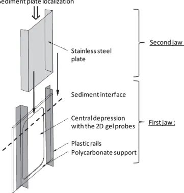
For the two-dimensional sampling, we used a “jaw device”, composed of two main parts (jaws; Fig. 1). The first jaw is a DET gel probe which samples the dissolved chemical species from the pore water at high resolution, whereas the second jaw samples a 2 cm thick slice of the adjacent sediment, from which we subsampled 1 cm3aliquots for foraminiferal anal-ysis. The first jaw is a 250 mm × 200 mm × 2 mm polycar-bonate plate with a central depression of 1 mm that holds a 2-D gel probe. The probe is made of two layers: (1) a 180 mm × 97 mm × 0.92 mm polyacrylamide thin film pre-pared and rinsed with Milli-Q water (Krom et al., 1994) which reaches equilibrium in a few hours once incubated (called “2-D DET gel”) and (2) a PVDF porous (0.2 µm) membrane to protect the gel and prevent it from falling out of the depression and control diffusion. The 2-D DET gel was prepared and mounted less than 1 week before sampling, conserved in a wet clean plastic bag, and then de-aerated by N2bubbling for about 6 h before deployment. The sam-pler was deployed into the sediment at low tide. On both lateral sides of the central depression (Fig. 1), plastic rails (2 cm high) were fixed in order to guide the second jaw to slide along the plate. The second jaw is a stainless steel plate (1.5 mm thick) bent on both sides. After equilibration (5 h) of the 2-D gel, the second jaw was inserted along the guides of the first jaw and the whole device was gently pulled out of the sediment. Once onshore, the 2-D gel was separated from the sediment, covered with a plastic-coated aluminium plate and stored in an icebox with dry ice pellets (Cesbron et al., 2014) until final storage in a freezer (−18◦C).
The sediment plate was manually cut (with stainless steel trowels) within 30 min in 1 cm3 cubes for a sur-face of 8 cm × 8 cm. The resulting sampling map is pre-sented in Fig. 2 together with the 1-D sampling scheme of foraminifera. Next, these sediment cubes were labelled with CTG so that living foraminifera could be recognized (as for the core slices; see Sect. 2.2). Considering an error of 1 mm for each cut, the volume uncertainty was ∼ 14 %, except for surface samples where the microtopography of the sediment surface considerably increases volume uncertainty.
The 2-D DET probe was analysed in order to obtain the concentrations of dissolved iron and dissolved reactive phos-phate (DRP) (Cesbron et al., 2014). After thawing at ambi-ent temperature, the sample gel was quickly recovered by a reactive gel equilibrated in specific colorimetric reagents. Twenty-five minutes after contact, a photograph (reflectance analysis) of superposed gels was taken with a hyperspec-tral camera (HySpex VNIR 1600) and analysed. The res-olution (surface area of pixels) was 211 µm × 216 µm. The estimated incertitude is 10 % for iron and 11 % for DRP. For further details, see Supplement S3. To compare the geo-chemical species distribution (at submillimetre resolution) and foraminiferal density (at centimetre resolution), an R
Polycarbonate support Central depression with the 2D gel probes Plastic rails Stainless steel plate Sediment interface First jaw : Second jaw : Sediment plate localization
Figure 1. Schematic view of the “jaw device” for simultaneous
sampling of sediment and porewater.
code was written that allowed for the downscaling of chemi-cal resolution from 0.2 mm to 1 cm.
2.4 Statistical analyses
The patchiness effect or autocorrelation, interpreted as the fact that the density of one square depends on its neigh-bours, was explored using spatial correlograms built using Moran’s index (I ), computed with R (package “spdep”, fol-lowing Fortin and Dale, 2005; Bivand et al., 2008; Legendre and Fortin, 2010; Borcard et al., 2011; Eq. 1). This index was applied to benthic meiofauna by Blanchard (1990) and Eck-man and Thistle (1988) and to foraminifera by. Hohenegger et al. (1993). This index calculates the similarity of pair val-ues for one neighbourhood – a neighbourhood being defined by a weight (wi,j) function of the distance (d) between pairs.
I (d) = n P i,j wi,j(d) (xi− ¯x) (xj− ¯x) s n P i (xi− ¯x)2 × n n P i,j wi,j(d) (1)
Here, the n = 40 cubes used for Moran’s index have neigh-bourhoods defined as cubes in direct contact (four neighbours per sample with a weight of 1 and the others have 0, also known as “rook connectivity”; Fortin and Dale, 2005). With this configuration, Moran’s index is −1 for a contrasted or-ganization (perfect negative correlation between neighbours) and +1 in the case of grouped organization (perfect
posi-A B C 1 2 3 4 5 6 7 8 D E F G H
A Plexiglas core-slicing B « jaw device » sampling
Figure 2. Sediment sampling methodology for living foraminiferal analyses. (a) Usual 1-D hand coring and layer slicing. (b) Sediment plate
sampling with the second jaw of the “jaw device” (Fig. 1) and representation of the sediment cubic slicing.
tive correlation between neighbours). A value close to zero (I0=(n −1)−1) corresponds to no organization or random distribution. The correlogram plots Moran’s index versus the order of the neighbours (o.n.). A decrease in the Moran’s in-dex from positive to negative values characterizes a patchy distribution. The characteristic length of the patchiness is de-fined as the order of neighbours when Io.n.=0 (Legendre and Fortin, 1989). Two-dimensional non-random organiza-tion was tested with the alternative hypothesis: Io.n.> I0. The second test examines if there is a preferential direction in the organization (isotropy). Again, the alternative hypothesis for Moran’s index, Io.n.> I0, is used, restricting the distance to the tested dimension (vertical or horizontal). Thus, in our case, each sample was compared only with its lateral or ver-tical neighbours (i.e. two neighbours per test).
3 Results
3.1 1-D geochemical features
Figure 3 shows both solid and dissolved chemical species obtained from the dedicated cores. Total organic carbon (Corg, black circles, Fig. 3a) decreased from 2700 to 1900 µmol g(dry sediment)−1in the first centimetre, then in-creased sharply until 1.5 cm depth, and finally dein-creased
pro-gressively from 2700 to 2400 µmol g(dry sediment)−1at 5 cm depth. Salinity (Fig. 3a) ranges from 7.5 to 1.7 with an off-set of ∼ 2 between replicates and a decrease of ∼ 3 in the first 13 cm. Figure 3b shows the vertical distribution of dis-solved oxygen. The 3 profiles shown (out of 18) are consid-ered representative of the lateral variability in the sediment. Most of the oxygen concentration profiles show the exponen-tial trend typical for undisturbed marine sediments (two pro-files in Fig. 3b, with light-grey and white diamonds; Revs-bech et al., 1980; Berg et al., 1998). However, one-third of the O2profiles diverged from the exponential model, show-ing an interruption of the decreasshow-ing trend, or even a local increase, at depth (e.g. the profile with dark-grey diamonds represented in Fig. 3b). The oxygen penetration depth (OPD) remained relatively constant around 2.0 mm (SD = 0.2 mm,
n =18) despite this heterogeneity.
Figure 3c, d and e show the distribution of manganese, iron and phosphorus, respectively, both in the dissolved phase (grey and open diamonds) and in the easily reducible solid phases (black circles, extracted by ascorbate leaching; An-schutz et al., 2005; Hyacinthe et al., 2006). Extracted man-ganese (mainly (hydr)oxide, black circles in Fig. 3c) showed a strong enrichment of the easily reducible solid phase (until 13 µmol g(dry sediment)−1)in the first 2 mm, where an im-portant upward diminution was visible in both replicates of
0.00 0.05 0.10 0.15 0.20 0.25 0.30 0 100 200 300 [O2] (µmol L-1) 0 5 10 0 2 4 6 8 10 12 0 2000 4000 Salinity D ep th (c m) Corg (µmol g-1) 0 50 100 0 2 4 6 8 10 12 0 10 20 [Mn]dissolved(µmol L-1) De p th (c m) 0 500 1 000 0 2 4 6 8 10 12 0 100 [Fe]dissolved (µmol L-1) 0 200 400 0 2 4 6 8 10 12 0 10 20 [P]dissolved(µmol L-1)
A B C [Mn]asc (µmol g-1)D [Fe]asc (µmol g-1) E [P]asc (µmol g-1)
Figure 3. 1-D geochemical features. (a) Vertical profile of total solid organic carbon (filled circles, uncertainty smaller than symbol size) and
profiles of salinity (white and grey diamonds). (b) Typical profiles of dissolved oxygen; the profile with dark-grey diamonds is considered bioturbated. (c, d, e) Vertical profiles of manganese (c), iron (d) and phosphorus (e) in dissolved (white and grey diamonds for DET replicates) and reactive solid phase (ascorbate-leached) from the core (black circles).
the dissolved phase (grey and open diamonds in Fig. 3c). Below, the solid phase showed a slightly decrease from 7.9 to 5.6 µmol g(dry sediment)−1until 5 cm depth. The dis-solved manganese concentration decreased between 4 and 9 cm depth in both replicates (from 70 to 30 µmol L−1). In the solid phase, iron, phosphorus and manganese are strongly correlated when the surface sample is not consid-ered (r2=0.70 between iron and manganese and r2=0.55 between and iron and phosphorus). Profiles of dissolved iron and phosphorus are also strongly correlated (r2=0.90, slope = 1.87 and r2=0.47, slope = 1.31 for replicates A and B). Iron and phosphorus were remobilized, and there-fore appeared in the dissolved phase, between 1 and 9 cm. Both replicates of dissolved iron showed the same four well-described maxima (at least six samples for each maximum) at 2.3, 3.3, 5.9 and 7.3 cm depth but with different concen-trations. In replicate A (open diamonds) these maxima have 5 times higher iron concentrations (up to 700 µmol L−1)than in replicate B.
3.2 Visual features on the sediment plate
Figure 4a shows the sediment slice obtained from the “jaw device” facing the 2-D DET gel. In order to facilitate the de-scription, the figures were subdivided into centimetre squares labelled with letters for the horizontal position and numbers for the vertical position. The black rectangle corresponds to the 2-D DET gel position, the blue rectangle to the gel signal exploited and the red rectangle to the 2-D foraminiferal sam-pling. Burrows parallel to the cutting plan are visible over their entire length. When perpendicular to the cutting plan, they appear as a dark hole (B14 in Fig. 4a). Figure 4b
summa-rizes burrow distributions superimposed on a picture of the gel after equilibration with the colorimetric reagents (pink coloration corresponds to iron and blue to dissolved reactive phosphorus (DRP)). Five burrows were visibly connected to the sediment surface; their traces mostly extended vertically down to 10 cm depth, where their track is lost. Between 10 and 15 cm depth, visible burrow density decreased. Below 15 cm depth, burrows were rarely observed and the sediment was dark (Fig. 4a). During slicing of the sediment plate, living polychaetes (Hediste diversicolor) were observed in some burrows.
3.3 2-D DET gel
Figure 5 shows the two-dimensional data sets, with the dis-tribution of dissolved phosphorus (Fig. 5a) and iron (Fig. 5b) obtained from the 2-D DET gel. For comparison, burrow distribution is shown in Fig. 5a. Dissolved iron and phos-phorus both appeared a few millimetres below the sediment– water interface. They are positively correlated for the whole plate (r2=0.59, slope = 2.7). Despite their patchy distribu-tion, both species can be observed along the entire length of the gel probe (i.e. 17 cm depth). A main feature was the occurrence of two prominent vertical structures enriched in dissolved iron and phosphorus (A-B/6–9 and F-G/5–14; Fig. 5). The highest concentrations, of about 170 and 50 µmol L−1 for iron and phosphorus, respectively, were found within the structure at the right (squares F/8–9). In the structure on the left (A/6–8), iron and phosphorus maxima were around 120 and 25 µmol L−1, respectively.
Most burrows seem to impact the iron concentration. For example, burrows 1, 3 and 5 clearly correspond (in the
A B C D E F G H 1 2 3 4 5 6 7 8 9 10 11 12 13 14 15 16 17 A B C D E F G H 1 2 3 4 5 6 7 8 9 10 11 12 13 14 15 16 17 1 2 3 4 5
A Sediment plate B 2D gel after colorimetric reactions
Figure 4. (a) Picture of the sediment plate before cube slicing for foraminiferal analysis (sediment–water interface at the top). (b) Picture
of the analysed gel after colorimetric reactions: dissolved iron shown in dark pink and dissolved phosphorus in turquoise (burrows superim-posed). The black rectangle corresponds to the gel limit, the blue rectangle to the limit of available data set of dissolved iron and phosphorus and the red rectangle to the limit of the available data set of foraminiferal distribution.
C A. tepida (ind cm-3) D ep th (cm ) A B C D E F G H A B C D E F G H 1 2 3 4 5 6 7 8 9 10 11 12 13 14 15 16 17 D e p th (c m ) Width (cm) Width (cm) Width (cm) A B C D E F G H 1 2 3 4 5 6 7 8 A DRP (µmol L-1) B Dissolved iron (µmol L-1)
Figure 5. (a, b) Two-dimensional concentrations after numerical analysis of dissolved reactive phosphorus (DRP) and dissolved iron. The
distribution of burrows is shown on the DRP plot. Red lines represent the boundary of foraminiferal analysis. (c) 2-D distribution of A. tepida densities from the sediment plate with burrow distribution.
first 4 cm) to a drastic decrease in or even disappearance of dissolved iron, whereas other burrows seem to corre-spond to a dissolved iron enrichment (F-G/5–9). However, some centimetre-sized patches (e.g. A-B/6–9, H-G/8–9 and F-G/17) seem to be unrelated to burrow structures. Below
15 cm depth, the sediment was dark and dissolved iron gen-erally decreased, whereas DRP increased.
3.4 Living foraminiferal distribution
Figure 5c shows the distribution of CTG-labelled Ammonia
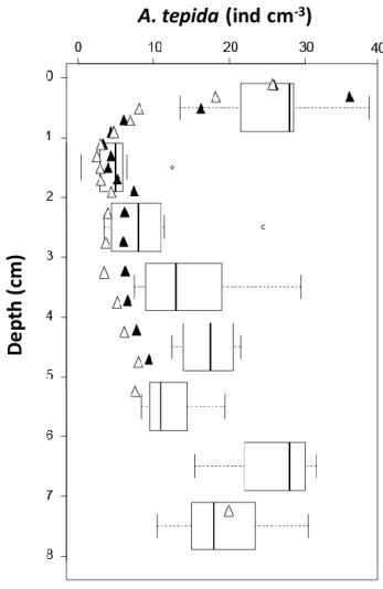
tepida determined for 1 cm3samples in the sediment facing the 2-D DET gel. The analysis of living foraminifera in the 64 cubes (8 cm width × 8 cm depth) takes roughly the same time as the analysis of one core of 8.2 cm diameter (until 5 cm depth). Ammonia tepida was by far the dominant species, ac-counting for 92 % of the total assemblage. The second most frequent species, Haynesina germanica, represented 5 %, but its low density (mostly 0, 1 or 2 individuals per cubic cen-timetre) was not sufficient to support a serious discussion. For this reason the data relative to this species are omitted from the present paper. A. tepida density ranged from 0 to 38 individuals cm−3with important lateral and vertical vari-ability. The relative standard deviation (RSD) calculated for each row is, on average, 45 %, whereas for each column the RSD is 60 %, suggesting a slightly more pronounced verti-cal organization. This is confirmed by the stratification of the richest samples (≥ 27 individuals cm−3), which were found in the topmost centimetre and below 6 cm depth, whereas the poorest samples (≤ 5 individuals cm−3)were found between 1 and 3 cm depth. Each row from the 2-D distribution can be represented by a box-and-whisker plot (Fig. 6). The re-sults confirm a three-step pattern with high densities at the surface (13 to 38 individuals cm−3), lower density between 1 and 3 cm depth (0–12 individuals cm−3and one outlier at 24 individuals cm−3)and increasing values below 3 cm (7 to 31 individuals cm−3).
This vertical pattern is also visible in the two stud-ied sediment cores (Fig. 6): high densities of A. tepida (26 ± 0 individuals cm−3) are observed in the first 2 mm, with a rapid decrease to minimal densities in the 1.0–1.2 cm layer (3 ± 0 individuals cm−3), followed by a progressive, somewhat irregular increase until 9 ± 0 individuals cm−3 be-low 2 cm depth to 8 cm depth. Despite the different vertical sampling resolution, the densities observed in the cores are in agreement with the average densities observed in the sed-iment slice cubic samples.
4 Discussion
4.1 A methodological improvement to characterize heterogeneity
Here, we present for the first time a methodology allowing the simultaneous study of the vertical and horizontal hetero-geneity of dissolved chemical species and living foraminifera (determined by CTG labelling) in the first 8 cm of the sedi-ment. Figure 6 compares the vertical density distribution of
A. tepida between the cores (triangles) and the jaw device
(box-and-whisker plots), sampled a few decimetres apart. Despite the different vertical sampling resolution, the den-sities observed in the cores (sampling surface of 53 cm2) are
D
e
p
th
(
cm
)
A. tepida (ind cm
-3)
Figure 6. Vertical comparison of A. tepida densities from the two
cores (filled and open triangles) and the “jaw device” sampling (each box plot represents the distribution of one layer; bars are first and third quartiles for the boxes length and whiskers are below 1.5 interquartiles; open circles are outliers).
in agreement with the average densities observed in the sedi-ment slice samples (sampled with the “jaw device”, sampling surface of 8 cm2). This similarity suggests a limited horizon-tal heterogeneity of A. tepida at the decimetre scale, although it is impossible to draw firm conclusions on the basis of only three samples (the two cores and the jaw device).
The jaw device (box plot whiskers, Fig. 6) reveals a hetero-geneous horizontal distribution at the centimetre scale. The centimetre-scale heterogeneity is quantified by calculating the Moran’s index that estimates the characteristic length of foraminiferal niches. Figure 7 shows Moran’s index correlo-grams applied between 3 and 8 cm depth (suboxic sediment), where high densities of living foraminifera were observed. Figure 7a shows that the spatial organization of A. tepida is patchy at the centimetre scale (I1=0.24, p value = 0.013). For farther neighbours the Moran’s index values drop to zero, meaning random organization. Concerning vertical and hori-zontal heterogeneities, Moran’s index values for direct
neigh-bours are 0.02 and 0.47, with p values of 0.38 and 0.001, respectively. For second-order neighbours, values do not sig-nificantly differ from 0 in either direction (data not shown). This means that A. tepida specimens tend to be grouped in horizontal spots with a characteristic length of 1 to 2 cm.
Figure 7b shows the Moran’s index correlogram for iron at 1 cm scale resolution (phosphorus is similar and not shown). It shows strong patchiness (I1=0.7) for direct neighbours in either directions, with a characteristic length of 3–4 cm. The fact that the characteristic lengths of A. tepida (Fig. 7a) and dissolved iron (Fig. 7b) patches are longer than 1 cm suggests that the impact of different sampling thicknesses (roughly zero for dissolved iron compared to 1 cm for foraminifera) would not result in major bias. Moreover, this characteristic length is important as it likely corresponds to the character-istic length of the controlling mechanisms (Clark, 1985; Wu and Li, 2006). In fact, the difference in Moran’s index be-tween chemical species and the A. tepida density distribution suggests that not exactly the same mechanisms control these parameters. This is an unexpected result, since most concep-tual models explain benthic foraminiferal distribution in the sediment as a direct response to geochemical gradients, es-pecially oxygen and sulfide (Jorissen et al., 1998; Van der Zwaan et al., 1999; Fontanier et al., 2002; Langezaal et al., 2006; Langlet et al., 2013), which intimately control iron re-mobilization.
4.2 Factors generating chemical heterogeneity
The heterogeneity of geochemical patterns is mainly ex-plained by the availability of oxidants mineralizing or-ganic carbon. In the generally applied conceptual model of Froelich et al. (1979), organic matter remineralization is characterized by a succession of horizontal layers where spe-cific oxidants are used. Figure 3 confirms this theoretical vertical stratification: oxygen is rapidly consumed by respi-ration (about 2 mm depth, Fig. 3b), and thereafter reduced dissolved manganese appears (Fig. 3c). Dissolved iron ap-pears still deeper, with a first maximum at 2 cm depth. The slopes of the concentration profiles are steeper and the reac-tive solid phase (Fig. 3d and c) is more concentrated for iron than for manganese, suggesting a higher reactivity. However, the strictly vertical succession of redox layers is no longer respected in the deeper suboxic layers, as suggested by the presence of multiple maxima of iron (Fig. 3d) and by the high lateral heterogeneity observed in Fig. 5a and c. This high lat-eral heterogeneity cannot be explained by vertical diffusion of oxygen. It appears therefore that a strictly vertical strati-fication of redox zones, defining a similar foraminiferal mi-crohabitat succession, is not a reasonable assumption for our study area.
4.2.1 Macrofaunal impact on heterogeneity
Macrofauna is assumed to be the most important cause of chemical heterogeneity at a scale of 0.01 cm (roughly the foraminiferal scale) to 100 cm (station scale), because of its ability to reorganize the sediment. In this way, macrofauna determines whether other factors can impact the heterogene-ity of dissolved iron and/or A. tepida. Macrofauna modi-fies (i) the sediment texture/composition (burrow walls or faecal pellets); (ii) the redox conditions, by ventilation of their burrows with oxygenated water (bioirrigation); and (iii) particle arrangement, by crawling or burrowing (biomixing) (Meysman et al., 2006). The efficiency of biomixing to ho-mogenize the sediment mainly depends on two aspects (see Wheatcroft et al., 1990, or Meysman et al., 2010a, for a more detailed discussion):
1. TS1The biomixing species assemblage. At the Les Brillantes mudflat, the main macrofaunal species are
Hediste diversicolor (630 individuals m−2) and
Scro-bicularia plana (70 individuals m−2; I. Métais, personal communication, 2015). H. diversicolor is a gallery diffusor (particle mixing due to burrowing activity), whereas S. plana is an epifaunal biodiffusor (particles are mixed in a random way over short distances along the surface; e.g. François et al., 2002; Kristensen et al., 2012). These two species generate homogeneity or het-erogeneity according to the second criterion. See below.
2. The relation between the average time of existence of the studied objects (here foraminifera and dissolved iron) in the bioturbated area and the average time between two bioturbation events. Frequent bioturba-tion events generate efficient mixing (homogeneity), whereas rare bioturbation events generate heterogene-ity. The average time between two bioturbation events is estimated to be days to months by tracer modelling (Wheatcroft et al., 1990; Meysman et al., 2003, 2008), while the longevity of foraminifera in suboxic environ-ments is estimated to be roughly 1 year (Langlet et al., 2013; Nardelli et al., 2014). The mean residence time of iron in the dissolved phase is estimated between 2 and 3 days (Thibault de Chanvalon et al., in preparation). Therefore, biomixing should generate a homogeneous distribution of foraminiferal density distribution, con-trasting with a heterogeneous distribution of dissolved iron (and DRP). The different time spans also suggest that most of the living foraminifera were already present in the suboxic sediment before the visible (most recent) burrows were created. Conversely, the heterogeneity of the dissolved chemical species should be directly re-lated to biomixing and to others factors that have not been homogenized by biomixing, i.e. with a short time of existence in suboxic environments.
note the remarks at the end of the manuscript.
Order of neighboƵrs (cm scale)
90 115 132 131 110 * 67Moran’s Index correlogram for A.tepida
A
Mor
an’
s
Inde
x
* 90 * 115 132 131 * 110 * 67Moran’s Index correlogram for [Fe]dissolved
Order of neighboƵrs (cm scale)
B
Mor
an’
s
Inde
x
Figure 7. Moran’s index correlograms for 3 to 8 cm depth. (a) Moran’s index correlogram for A. tepida with a 1 cm resolution. (b) Moran’s
index correlogram for [Fe]dissolved with a 1 cm resolution. An asterisk indicates significant differences from zero; error bars are twice the standard deviation. The numbers are the number of pairs for each order of neighbours.
4.2.2 Geochemical impact of biogenic factors
The factors likely to generate chemical heterogeneity are (1) bioirrigation, which mainly causes an increase in oxidant availability (Aller and Aller, 1986; Aller, 2004; Arndt et al., 2013), and (2) biogenic particles (e.g. decaying macrofauna, faecal pellets), which cause an increase in labile carbon avail-ability. Dissolved iron shows two opposite types of behaviour (Aller, 1982). (1) Iron precipitates as a hydroxide when the oxidative state of the pore water surrounding active burrows increases (Meyers et al., 1987; Zorn et al., 2006; Meysman et al., 2010b). This is confirmed by visible burrows in Fig. 5 in which both dissolved iron and DRP are depleted (Fig. 4, numbers 1, 3, 5 (above 6 cm depth) and burrows in B-D/13, E/9–11, G-H/10–15 and A-B/9). These structures are mainly vertical and have a length often exceeding 3 cm, in agreement with the Moran’s index correlogram. Conversely, within the long burrow F-G/5–9, dissolved iron is enriched, indicating that this burrow is abandoned and no oxygen renewal occurs. This feature was also observed for some burrows by Zhu and Aller (2012) and Cesbron et al. (2014). (2) Dissolved iron is produced by anaerobic respiration where biogenic parti-cles increase labile carbon availability, and thereby decrease the oxidative state of surrounding pore waters (Robertson et al., 2009; Stockdale et al., 2010). The geometry and isolation from visible burrows of patches A/7–8, G-H/8–9 and F-G/17 in Fig. 5a and b suggest that they could represent centimetre-wide labile organic matter patches. We hypothesize that these patches correspond to intense remineralization of biogenic particles that dissolves iron oxides.
4.3 Mechanisms controlling the A. tepida distribution Figures. 5c and 6 clearly describe a three-step pattern in the distribution of A. tepida, with high densities at the surface, low densities between 1 and 3 cm depth, and a somewhat sur-prising increase below (in suboxic sediments). A similar pat-tern has been reported, but not discussed, for other intertidal environments (Alve and Murray, 2001; Bouchet et al., 2009). In our study, the consistency of the eight vertical columns from the plate sampling confirms the robustness of this pat-tern, and the two-dimensional approach reveals an organiza-tion of A. tepida in centimetre-wide patches in the suboxic sediment. The next subsections discuss possible mechanisms that could explain these features, especially in the suboxic environment, where active burrows (supporting biomixing and bioirrigation) and biogenic particles have been identified as factors likely to generate such heterogeneity.
4.3.1 Foraminiferal metabolism
Generally, aerobic metabolism is considered the dominant mechanism in oxic conditions since it is energetically most efficient. In fact, Figs. 5c and 6 clearly describe maximal den-sities of A. tepida at the sediment surface (0–2 mm depth) and low densities below (6–18 mm depth). This strong gradi-ent of A. tepida density highlights the presence of a contin-uously oxygenated microhabitat enriched in organic matter (see TOC and O2profiles, Fig. 3a–b) close to the sediment– water interface, favourable for A. tepida. Energetic consid-erations and some observations that report a strong seasonal variability in the oxic zone (Moodley, 1990; Barmawidjaja et al., 1992) led to the assumption that foraminifera reproduce preferentially in the oxic layer (de Stigter et al., 1999;
Berke-ley et al., 2007). Together, these factors explain the maximum density in the surface layer.
Since the work of Richter (1961), numerous publications have reported living benthic foraminifera in suboxic sedi-ment layers (Jorissen et al., 1992; Moodley and Hess, 1992; Bernhard and Sen Gupta, 2003). For intertidal environments, studies have reported living (rose bengal stain) foraminifera in subsurface environments since the 1960s (e.g. Buzas, 1965; Steineck and Bergstein, 1979). Several in situ (Gold-stein et al., 1995; Bouchet et al., 2009) and laboratory (Moodley and Hess, 1992; Moodley et al., 1998; Pucci et al., 2009; Nardelli et al., 2014; Nomaki et al., 2014) studies with
A. tepida have also reported survival, activity and even
calci-fication in suboxic conditions. Anaerobic metabolism would be a logical mechanism to explain the presence of large amounts of living foraminifera in suboxic layers. Complete or partial (with endo- and/or ectobionts; Bernhard and Alve, 1996) denitrification co-occurring with nitrate storage has been demonstrated for some foraminiferal taxa (Risgaard-Petersen et al., 2006). Nomaki et al. (2014) suggested denitri-fication by endobionts for A. tepida. However, denitridenitri-fication has not been measured in A. tepida, and only very low intra-cellular nitrate concentrations were found (Pina-Ochoa et al., 2010; Geslin et al., 2014). It appears therefore unlikely that the abundance of living A. tepida in deeper suboxic layers can be explained by active colonization.
4.3.2 Burying and burrow microenvironment
It is clear that biomixing is a likely mechanism to explain the introduction of foraminifera in deeper sediment layers by passive transport (Alve and Bernhard, 1995; Goldstein et al., 1995; Moodley et al., 1998; Saffert and Thomas, 1998; Alve and Murray, 2001; Jorissen, 2003). However, the spatial distribution resulting from this passive transport has never been well described, or modelled. According to the theory of biomixing, we suggest that the vertical distribution of A.
tep-ida can be approached with a diffusion model, which should
lead to an exponential downward decrease, with the slope as a function of the mortality rate. A. tepida is possibly able to survive in suboxic environments using an intermittent aero-bic metabolism, using the oxygen that can be occasionally available due to bioirrigation (Fenchel, 1996; Wang et al., 2001; Wenzhofer and Glud, 2004; Pischedda et al., 2012). Their activity should progressively decrease once oxygen is depleted; Phipps (2012) suggested that they could finally be immobilized before dying as a result of a prolonged absence of oxygen supply. We think that repeated introduction by macrofaunal bioturbation, followed by reduced metabolic ac-tivity, leading to immobilization, is the most likely mecha-nism to explain the high abundances of living foraminifera in suboxic sediments.
Figures 4a and 5b show no relation between visible bur-rows and living A. tepida. This result is in agreement with the different timescales of the foraminiferal lifespan and the
burrows, and with the idea that biomixing homogenizes the
A. tepida density. It also suggests that the oxygen obviously
brought by formation of new burrows is consumed too fast to allow all infaunal A. tepida to migrate to these active bur-rows. Thus, recent burrow walls are apparently not colonized by specimens of A. tepida already present in the suboxic sed-iment. Our observations contrast with earlier studies, show-ing increased foraminiferal densities (up to 300 times higher than in the surrounding sediment, rose bengal staining) in burrow walls. For example, data from burrows of Amphicteis sp. at 4800 m depth (Aller and Aller, 1986), of Echiurus
echi-urus at 42m depth (Thomsen and Altenbach, 1993), and of Pestarella tyrrhena in intertidal sand flats (Koller et al., 2006)
all presented high foraminiferal densities. The observed dif-ferences could be due to the fact that burrows of various macrofaunal taxa may represent very different environmental conditions and possibly due to a difference in sampling scale, since Thomsen and Altenbach (1993) and Koller et al. (2006) applied an irregular millimetre sampling around burrows. To summarize, macrofaunal activity would explain transport to and survival in suboxic layers. However, it does not explain the density minimum at 1–3 cm depth.
4.3.3 Sensitivity to geochemical gradients
We think that the most probable explanation for the 1–3 cm density minimum of A. tepida is an active upward migra-tion of the specimens, back to the sediment surface, before they are completely immobilized by a lack of oxygen and a strongly lowered metabolism. Numerous studies have al-ready reported that vertical migration of foraminifera allows them to move to more hospitable environments (Jorissen, 1988; Van der Zwaan and Jorissen, 1991; Alve and Bern-hard, 1995; Moodley et al., 1998; Gross, 2000; Langezaal et al., 2003; Geslin et al., 2004; Ernst et al., 2005). In an experiment in which populations of Haynesina germanica were uniformly mixed in a 6 cm sediment column, Ernst et al. (2006) saw a clear migration back to the surface for the foraminifera living between 1 and 3 cm depth, and sug-gested that foraminifera living at greater depth were unable to do so. Similarly, Hess et al. (2013) showed that benthic foraminifera are able to migrate through suboxic sediment to reach oxic sediments over a maximal distance of a few centimetres. Active migration towards directly detected oxy-gen or organic matter over distances beyond 1 cm seems im-probable, since this distance is much higher than the typical pseudopodial length (about 1 cm; see Travis and Rabalais, 1991). However, as described above, the presence of oxygen could be indirectly detected by other geochemical gradient (e.g. NO−3, Mn2+or Fe2+, dissolved organic carbon, pCO2). However, when gradients generated by the oxygen front are imperceptible for A. tepida, because they are living too deep in the sediment, or when such gradients are hidden by other sources of geochemical gradients (as organic-rich patches), this upward migration could no longer occur. This could
ex-plain why, below 3 cm depth, A. tepida remains in the deeper sediment layer after being transported there accidentally.
However, the organization of the foraminiferal in 1–2 cm wide horizontal patches identified by Moran’s index suggests that A. tepida detects not only vertical geochemical gradi-ents but probably also lateral gradigradi-ents around degrading bio-genic particles. The characteristic length of patches corre-sponding to biogenic particles identified by dissolved iron maxima (A/7–8, G-H/8–9 and F-G/17 in Fig. 7c and d; see Sect. 4.2.2) is in agreement with the characteristic length of foraminiferal density maxima. For instance, in the first 8 cm, the two identified biogenic particles patches (A/7–8, G-H/8– 9 in Fig. 5b) both correspond to a higher density of A.
tep-ida (28/19 and 21/30 individuals cm−3on average for A/7–8 and G-H/8, respectively, Fig. 5c). In agreement with these re-sults and despite a lowered metabolism, we hypothesize that foraminifera could move towards patches of labile organic matter even in deeper suboxic layers. Nevertheless, a bet-ter identification of labile carbon patches, replicate sampling with the here-developed strategy, and experimental studies with artificial geochemical gradients are necessary to confirm our hypotheses about the behaviour of A. tepida in suboxic environments.
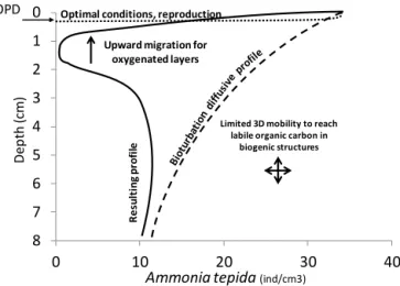
To summarize, we suggest that the distribution of A.
tep-ida can be interpreted as the result of not less than five
in-teracting mechanisms (Fig. 8). (1) High foraminiferal den-sities at the surface are the result of the presence of abun-dant labile organic matter and reproduction in the oxygenated layer (Sect. 4.3.1); (2) downward transport by macrofaunal biomixing introduces living foraminifera into deeper sedi-ment layers (Sect. 4.3.2); (3) in the first 3 cm foraminifera are capable to migrate back to the oxygenated, organic-rich surface layers once they detect redox gradients, whereas in deeper sediment layers, they are no longer capable to find their way back to the superficial oxygenated layer (Sect. 4.3.3); (4) after a prolonged presence in suboxic con-ditions, foraminifera lower their metabolism and become inactive; and (5) foraminifera can be temporarily remobi-lized during intermittent bioirrigation events, and can eventu-ally migrate towards organic-rich microenvironments in their vicinity (Sect. 4.3.3). A better identification of labile carbon patches – for example based on alkalinity (Bennett et al., 2015), pCO2(Zhu et al., 2006; Zhu and Aller, 2010) or dis-solved organic carbon – should allow the interpretation to be taken further.
5 Conclusions
We present a new, simple and robust sampling protocol for obtaining the 2-D distribution of benthic foraminifera com-bined with the 2-D distribution of geochemical species, in this case dissolved iron and phosphorus. This technique al-lows visual observation of burrow features. Geochemical fea-tures allowed us to recognize active burrows (with minimal
0 1 2 3 4 5 6 7 8 0 10 20 30 40 D ep th (c m )
Ammonia tepida (ind/cm3)
OPD Optimal conditions, reproduction
Upward migration for oxygenated layers
Limited 3D mobility to reach labile organic carbon in
biogenic structures R e su lt in g p ro fi le
Figure 8. Putative mechanisms explaining the A. tepida density
pro-file (OPD: oxygen penetration depth).
dissolved concentrations) and to determine that areas of dis-solved iron and phosphorus enrichment do not always rep-resent abandoned burrows. Our observations on an estuarine mudflat showed an important density of A. tepida in suboxic environments with a characteristic length of patches of 1 to 2 cm. Surprisingly, no direct relation was found between ac-tive burrows and the A. tepida distribution. However, an en-richment of A. tepida was observed in some areas where dis-similatory iron reduction was intense, suggesting that, even in suboxic environments, there is a relation between the spa-tial distribution of A. tepida and labile organic matter rem-ineralization. Our results show that the new sampling strat-egy proposed here can yield important new insights into the functioning of suboxic environments in estuarine mudflats.
The Supplement related to this article is available online at doi:10.5194/bg-12-1-2015-supplement.
Acknowledgements. This study is part of the RS2E – OSUNA project funded by the Région Pays de la Loire. Special thanks are due to Didier Jézéquel from IPGP who designed the “jaw device”. Thanks to Clement Chauvin, Cyrille Guindir, Hélène Koroshidi and Eve Chauveau for their support in the field and laboratory. We thank the three editorial reviewers, whose comments helped us in improving our manuscript.
References
Aller, J. Y. and Aller, R. C.: Evidence for localized enhancement of biological associated with tube and burrow structures in deep-sea sediments at the HEEBLE site, western North Atlantic, Deep-Sea Res. Pt. A, 33, 755–790, 1986.
Aller, R. C.: The Effects of Macrobenthos on Chemical Properties of Marine Sediment and Overlying Water, in: Animal-Sediment Relations, edited by: McCall, P. L. and Tevesz, M. J. S., Springer US, 53–102, 1982.
Aller, R. C.: Conceptual models of early diagenetic processes: The muddy seafloor as an unsteady, batch reactor, J. Mar. Res., 62, 815–835, 2004.
Alve, E. and Bernhard, J. M.: Vertical migratory response of ben-thic foraminifera to controlled oxygen concentrations in an ex-perimental mesocosm, Oceanogr. Lit. Rev., 42, 137–151, 1995. Alve, E. and Murray, J. W.: Temporal Variability in Vertical
Distri-butions of Live (stained) Intertidal Foraminifera, Southern Eng-land, J. Foraminifer. Res., 31, 12–24, 2001.
Anschutz, P., Zhong, S., Sundby, B., Mucci, A., and Gobeil, C.: Burial efficiency of phosphorus and the geochemistry of iron in continental margin sediments, Limnol. Oceanogr., 43, 53–64, 1998.
Anschutz, P., Dedieu, K., Desmazes, F., and Chaillou, G.: Specia-tion, oxidation state, and reactivity of particulate manganese in marine sediments, Chem. Geol., 218, 265–279, 2005.
Arndt, S., Jørgensen, B. B., LaRowe, D. E., Middelburg, J. J., Pan-cost, R. D., and Regnier, P.: Quantifying the degradation of or-ganic matter in marine sediments: A review and synthesis, Earth-Sci. Rev., 123, 53–86, 2013.
Barmawidjaja, D. M., Jorissen, F. J., Puskaric, S., and van der Zwaan, G. J.: Microhabitat selection by benthic Foraminifera in the northern Adriatic Sea, J. Foraminifer. Res., 22, 297–317, 1992.
Bennett, W. W., Welsh, D. T., Serriere, A., Panther, J. G., and Teas-dale, P. R.: A colorimetric DET technique for the high-resolution measurement of two-dimensional alkalinity distributions in sed-iment porewaters, Chemosphere, 119, 547–552, 2015.
Benyoucef, I.: Télédétection visible proche-infrarouge de la distri-bution spatio-temporelle du microphytobenthos estuarien, Ph.D. thesis, Université de Nantes, 4 August, 2014.
Benyoucef, I., Blandin, E., Lerouxel, A., Jesus, B., Rosa, P., Méléder, V., Launeau, P., and Barillé, L.: Microphytobenthos in-terannual variations in a north-European estuary (Loire estuary, France) detected by visible-infrared multispectral remote sens-ing, Estuar. Coast. Shelf Sci., 136, 43–52, 2014.
Berg, P., Risgaard-Petersen, N., and Rysgaard, S.: Interpretation of measured concentration profiles in sediment pore water, Limnol. Oceanogr., 43, 1500–1510, 1998.
Berkeley, A., Perry, C. T., Smithers, S. G., Horton, B. P., and Tay-lor, K. G.: A review of the ecological and taphonomic controls on foraminiferal assemblage development in intertidal environ-ments, Earth-Sci. Rev., 83, 205–230, 2007.
Berner, R. A.: Sedimentary pyrite formation, Am. J. Sci., 268, 1–23, 1970.
Bernhard, J. M. and Alve, E.: Survival, ATP pool, and ultrastructural characterization of benthic foraminifera from Drammensfjord (Norway): response to anoxia, Mar. Micropaleontol., 28, 5–17, 1996.
Bernhard, J. M. and Sen Gupta, B. K. S.: Foraminifera of oxygen-depleted environments, in Modern Foraminifera, Springer Netherlands, 201–216, 2003.
Bernhard, J. M., Ostermann, D. R., Williams, D. S., and Blanks, J. K.: Comparison of two methods to identify live benthic foraminifera: A test between Rose Bengal and CellTracker Green with implications for stable isotope paleoreconstructions, Paleo-ceanography, 21, PA4210, doi:10.1029/2006PA001290, 2006. Bivand, R., Pebesma, E., and Gomez-Rubio, V.: Applied Spatial
Data Analysis with R, Springer New York, New York, NY, 2008. Blanchard, G.: Overlapping microscale dispersion patterns of meio-fauna and microphytobenthos, Mar. Ecol. Prog. Ser., 68, 101– 111, 1990.
Borcard, D., Gillet, F., and Legendre, P.: Numerical Ecology with R, Springer New York, New York, NY, 2011.
Bouchet, V. M. P., Sauriau, P.-G., Debenay, J.-P., Mermillod-Blondin, F., Schmidt, S., Amiard, J.-C., and Dupas, B.: Influence of the mode of macrofauna-mediated bioturbation on the vertical distribution of living benthic foraminifera: First insight from ax-ial tomodensitometry, J. Exp. Mar. Biol. Ecol., 371, 20–33, 2009. Boudreau, B. P.: A method-of-lines code for carbon and nutrient diagenesis in aquatic sediments, Comput. Geosci., 22, 479–496, 1996.
Burdige, D. J.: 5.09 – Estuarine and Coastal Sediments – Coupled Biogeochemical Cycling, in: Treatise on Estuarine and Coastal Science, edited by: Wolanski, E. and McLusky, D., Academic Press, Waltham, 279–316, 2011.
Buzas, M. A.: On the spatial distribution of foraminifera:, Contrib. Cushman Found. Foraminifer. Res., 19, 1–11, 1968.
Buzas, M. A.: Spatial Homogeneity: Statistical Analyses of Unis-pecies and MultisUnis-pecies Populations of Foraminifera, Ecology, 51, 874–879, doi:10.2307/1933980, 1970.
Buzas, M. A., Hayek, L.-A. C., Reed, S. A., and Jett, J. A.: Foraminiferal Densities Over Five Years in the Indian River La-goon, Florida: A Model of Pulsating Patches, J. Foraminifer. Res., 32, 68–92, 2002.
Buzas, M. A., Hayek, L.-A. C., Jett, J. A., and Reed, S. A.: Pulsating Patches: History and Analyses of Spatial, Seasonal, and Yearly Distribution of Living Benthic Foraminifera, Smithson. Contrib. Paleobiology, 97, 1–91, 2015.
Cesbron, F., Metzger, E., Launeau, P., Deflandre, B., Delgard, M.-L., Thibault de Chanvalon, A., Geslin, E., Anschutz, P., and Jézéquel, D.: Simultaneous 2-D Imaging of Dissolved Iron and Reactive Phosphorus in Sediment Porewaters by Thin-Film and Hyperspectral Methods, Environ. Sci. Technol., 48, 2816–2826, 2014.
Clark, W. C.: Scales of climate impacts, Clim. Change, 7, 5–27, 1985.
Davison, W. and Zhang, H.: In situspeciation measurements of trace components in natural waters using thin-film gels, Nature, 367, 546–548, 1994.
Debenay, J.-P. and Guillou, J.-J.: Ecological transitions indicated by foraminiferal assemblages in paralic environments, Estuaries, 25, 1107–1120, 2002.
Debenay, J.-P., Bicchi, E., Goubert, E., and Armynot du Châtelet, E.: Spatio-temporal distribution of benthic foraminifera in rela-tion to estuarine dynamics (Vie estuary, Vendée, W France), Es-tuar. Coast. Shelf Sci., 67, 181–197, 2006.
de Stigter, H. C., van der Zwaan, G. J., and Langone, L.: Differ-ential rates of benthic foraminiferal test production in surface and subsurface sediment habitats in the southern Adriatic Sea, Palaeogeogr. Palaeoclimatol. Palaeoecol., 149, 67–88, 1999. Douglas, R. G.: Paleoecology of continental margin basins: a
mod-ern case history from the borderland of southmod-ern California, 1981.
Eckman, J. E. and Thistle, D.: Small-scale spatial pattern in meiobenthos in the San Diego Trough, Deep Sea Res. Part Oceanogr. Res. Pap., 35, 1565–1578, 1988.
Ernst, S., Bours, R., Duijnstee, I., and van der Zwaan, B.: Experi-mental effects of an organic matter pulse and oxygen depletion on a benthic foraminiferal shelf community, J. Foraminifer. Res., 35, 177–197, 2005.
Ernst, S. R., Morvan, J., Geslin, E., Le Bihan, A., and Jorissen, F. J.: Benthic foraminiferal response to experimentally induced Erika oil pollution, Mar. Micropaleontol., 61, 76–93, 2006.
Fenchel, T.: Worm burrows and oxic microniches in marine sedi-ments. 1. Spatial and temporal scales, Mar. Biol., 127, 289–295, 1996.
Fontanier, C., Jorissen, F. J., Licari, L., Alexandre, A., Anschutz, P., and Carbonel, P.: Live benthic foraminiferal faunas from the Bay of Biscay: faunal density, composition, and microhabitats, Deep-Sea Res. Pt. A, 49, 751–785, 2002.
Fortin, M.-J. and Dale, M. R. T.: Spatial analysis a guide for ecolo-gists, Cambridge University Press, Cambridge, NY, 2005. François, F., Gerino, M., Stora, G., Durbec, J., and Poggiale, J.:
Functional approach to sediment reworking by gallery-forming macrobenthic organisms: modeling and application with the polychaete Nereis diversicolor, Mar. Ecol. Prog. Ser., 229, 127– 136, 2002.
Froelich, P. N., Klinkhammer, G. P., Bender, M. L., Luedtke, N. A., Heath, G. R., Cullen, D., Dauphin, P., Hammond, D., Hartman, B., and Maynard, V.: Early oxidation of organic matter in pelagic sediments of the eastern equatorial Atlantic: suboxic diagenesis, Geochim. Cosmochim. Acta, 43, 1075–1090, 1979.
Geslin, E., Heinz, P., Jorissen, F., and Hemleben, C.: Migratory responses of deep-sea benthic foraminifera to variable oxygen conditions: laboratory investigations, Mar. Micropaleontol., 53, 227–243, 2004.
Geslin, E., Barras, C., Langlet, D., Nardelli, M. P., Kim, J.-H., Bon-nin, J., Metzger, E., and Jorissen, F. J.: Survival, Reproduction and Calcification of Three Benthic Foraminiferal Species in Re-sponse to Experimentally Induced Hypoxia, in: Approaches to Study Living Foraminifera, edited by: Kitazato, H. and Bernhard, J. M., Springer Japan, 163–193, 2014.
Goldstein, S. T., Watkins, G. T., and Kuhn, R. M.: Microhabitats of salt marsh foraminifera: St. Catherines Island, Georgia, USA, Mar. Micropaleontol., 26, 17–29, 1995.
Gross, O.: Influence of temperature, oxygen and food availability on the migrational activity of bathyal benthic foraminifera: evi-dence by microcosm experiments, in: Life at Interfaces and Un-der Extreme Conditions, edited by: Liebezeit, G., Dittmann, S., and Kröncke, I., Springer, the Netherlands, 123–137, 2000. Heinz, P. and Geslin, E.: Ecological and Biological Response of
Benthic Foraminifera Under Oxygen-Depleted Conditions: Evi-dence from Laboratory Approaches, in: Anoxia, edited by: Al-tenbach, A. V., Bernhard, J. M., and Seckbach, J., Springer, the Netherlands, 287–303, 2012.
Hess, S., Alve, E., Trannum, H. C., and Norling, K.: Benthic foraminiferal responses to water-based drill cuttings and natu-ral sediment burial: Results from a mesocosm experiment, Mar. Micropaleontol., 101, 1–9, 2013.
Hofmann, A. F., Soetaert, K., Middelburg, J. J., and Meysman, F. J. R.: AquaEnv?: An Aqua tic Acid–Base Modelling Env ironment in R, Aquat. Geochem., 16, 507–546, 2010.
Hohenegger, J., Piller, W., and Baal, C.: Reasons for spatial mi-crodistributions of foraminifers in an intertidal pool (northern Adriatic Sea), Mar. Ecol., 10, 43–78, 1989.
Hohenegger, J., Piller, W. E., and Baal, C.: Horizontal and vertical spatial microdistribution of foraminifers in the shallow subtidal Gulf of Trieste, northern Adriatic Sea, J. Foraminifer. Res., 23, 79–101, 1993.
Hyacinthe, C. and Van Cappellen, P.: An authigenic iron phosphate phase in estuarine sediments: composition, formation and chem-ical reactivity, Mar. Chem., 91, 227–251, 2004.
Hyacinthe, C., Anschutz, P., Carbonel, P., Jouanneau, J.-M., and Jorissen, F. J.: Early diagenetic processes in the muddy sediments of the Bay of Biscay, Mar. Geol., 177, 111–128, 2001.
Hyacinthe, C., Bonneville, S., and Van Cappellen, P.: Reactive iron(III) in sediments: Chemical versus microbial extractions, Geochim. Cosmochim. Acta, 70, 4166–4180, 2006.
Jézéquel, D., Brayner, R., Metzger, E., Viollier, E., Prévot, F., and Fiévet, F.: Two-dimensional determination of dissolved iron and sulphur species in marine sediment pore-waters by thin-film based imaging, Thau lagoon (France), Estuar. Coast. Shelf Sci., 72, 420–431, 2007.
Jorissen, F. J.: Benthic foraminifera from the Adriatic Sea: princi-ples of phenotypic variation, Utrecht Micropaleontol. Bull., 37, 1–174, 1988.
Jorissen, F. J.: Benthic foraminiferal microhabitats below the sediment-water interface, in Modern Foraminifera, Springer Netherlands, 161–179, 2003.
Jorissen, F. J., Barmawidjaja, D. M., Puskaric, S., and van der Zwaan, G. J.: Vertical distribution of benthic foraminifera in the northern Adriatic Sea: The relation with the organic flux, Mar. Micropaleontol., 19, 131–146, 1992.
Jorissen, F. J., de Stigter, H. C. and Widmark, J. G. V.: A concep-tual model explaining benthic foraminiferal microhabitats, Mar. Micropaleontol., 26, 3–15, 1995.
Jorissen, F. J., Wittling, I., Peypouquet, J. P., Rabouille, C., and Relexans, J. C.: Live benthic foraminiferal faunas off Cape Blanc, NW-Africa: Community structure and microhabitats, Deep Sea Res. Pt. A, 45, 2157–2188, 1998.
Koller, H., Dworschak, P. C., and Abed-Navandi, D.: Burrows of Pestarella tyrrhena (Decapoda: Thalassinidea): hot spots for Ne-matoda, Foraminifera and bacterial densities, J. Mar. Biol. Assoc. UK, 86, 1113–1122, 2006.
Kostka, J. E. and Luther III, G. W.: Seasonal cycling of Fe in salt-marsh sediments, Biogeochemistry, 29, 159–181, 1995. Kristensen, E., PenhaLopes, G., Delefosse, M., Valdemarsen, T.,
Quintana, C. O., and Banta, G. T.: REVIEW What is bioturba-tion? The need for a precise definition for fauna in aquatic sci-ences, Mar. Ecol. Prog. Ser., 446, 285–302, 2012.
Krom, M. D., Davison, P., Zhang, H., and Davison, W.: High-resolution pore-water sampling with a gel sampler, Limnol. Oceanogr., 39, 1967–1972, 1994.