Adaptive output-feedback control and applications to Very Flexible Aircraft

Adaptive Output-Feedback Control and Applications

to Very Flexible Aircraft

by

Zheng Qu

B.S., University of Michigan, Ann

Arbor

(2009)

S.M., University of Michigan, Ann Arbor (2010)

Submitted to the Department of Mechanical Engineering

in partial fulfillment of the requirements for the degree of

Doctor of Philosophy in Mechanical Engineering

at the

MASSACHUSETTS INSTITUTE OF TECHNOLOGY

June 2016

@

Massachusetts Institute of Technology 2016. All rights reserved.

Author

...

S ig

Depa

C ertified by ...

A ccepted by ...

iature redacted

rtment,f Mechanical Engineering

//

May 19, 2019

Signature redacted

Anuradha M. Annaswathy

Senior Research Scientist

Thesis Supervisor

Signature redacted

Rohan Abeyaratne

Chairman Department Committee on Graduate Students

MASSACHSTr1NTTT

JUN

0

2 2016]

LIBRARIES

ARCHVES

Adaptive Output-Feedback Control and Applications to Very

Flexible Aircraft

by

Zheng Qu

Submitted to the Department of Mechanical Engineering on May 19, 2016, in partial fulfillment of the

requirements for the degree of

Doctor of Philosophy in Mechanical Engineering

Abstract

Very Flexible Aircraft (VFA) corresponds to an aerial platform whose flight dynamics critically depends on its flexible wing shape, and has been investigated as a poten-tial solution to generate high-altitude low-endurance flights. The dominant presence of model uncertainties and potential actuator anomalies motivate an adaptive ap-proach for control of VFA. Another particular control challenge for VFA is that its flexible modes cannot be measured accurately, which necessitates an output-feedback multi-input multi-output (MIMO) control approach. The focus of this thesis is on an adaptive output-feedback controller for a generic class of MIMO plant models with an emphasis on the control of a VFA so as to execute desired flight maneuvers. The proposed adaptive controller includes a baseline design based on observers and pa-rameter adaptation based on a closed-loop reference model (CRM), and is applicable for a generic class of MIMO plants of arbitrary relative degree, and therefore the overall design is suitable for control in the presence of uncertainties in flexible effects, sensor dynamics, and actuator dynamics. In addition, the proposed controller can accommodate plant models whose number of outputs exceeds number of inputs. One major advantage of the proposed design is that the number of integrators required for implementation is significantly less than that of previous methods and therefore the controller can be implemented even for large-dimensional VFA models. Conditions are delineated under which asymptotic stability and command tracking can be guar-anteed, and the overall design is verified using realistic simulations on a high-fidelity VFA model with unknown varying wing shape and actuator anomalies.

Thesis Supervisor: Anuradha M. Annaswamy Title: Senior Research Scientist

Acknowledgments

I would like to extend my greatest gratitude towards my advisor, Anuradha

An-naswamy, for being tremendously supportive to my research. I would like to thank Eugene Lavretsky for insight and encouragement. I would also like to thank other members of my PhD committee, Kamal Youcef-Toumi and Domitilla Del Vecchio for valuable inputs.

This thesis is dedicated to my father and mother, whose wisdom and love indulge me until today. A quote from G. K. Chesterton would be appropriate to conclude this chapter of my life:

Fairy tales are more than true: not because they tell us that dragons exist, but because they tell us that dragons can be beaten.

Contents

1 Introduction

17

1.1 Large Dimension MIMO Systems ... 17

1.2 Very Flexible Aircraft . . . . 17

1.3 Linear Output-Feedback Control . . . . 18

1.4 Adaptive Output-Feedback Control . . . . 19

1.5 Relative Degree One Observer-Based Control Design . . . . 20

1.6 Higher Relative Degree Control Design . . . . 20

1.7 Nonsquare Plant Models . . . . 21

1.8 Synopsis of Thesis . . . . 21

1.9 Thesis Contributions by Chapter . . . . 22

2 Plant Model Description 25 2.1 A Class of Uncertain MIMO Plant Model . . . . 25

2.2 VFA M odel . . . . 28

2.2.1 3-Wing VFA Model . . . . 31

2.2.2 Vulture VFA Model. . . . . 32

3 Preliminaries 35 4 Relative Degree One Design 45 4.1 Relative Degree One Problem Statement . . . . 45

4.2 Relative Degree One Adaptive Control Design with SPR/LTR Prop-erties . . . . 47

4.2.1 Controller Structure . . . . 4.2.2 SPR/LTR Design . . . . 4.2.3 Design Procedure . . . . 4.2.4 Comparison with Other Adaptive Output-Feedback Controllers 4.3 Applications to VFA . . . .

4.3.1 Vertical Acceleration Tracking of 3-wing VFA . . . . 4.3.2 Vulture VFA Bank-To-Turn Control . . . .

5 Relative Degree Two Design

5.1 Relative Degree Two Problem Statement ...

5.2 Relative Degree Two Adaptive Control Design

5.2.1 Control Design . . . .

5.2.2 Underlying SPR Error Model . . . . .

5.2.3 Adaptive Law and Stability Proof . . .

5.2.4 Design Procedure . . . .

5.3 With Negligible Actuator Dynamics . . . .

5.4 Applications to VFA . . . .

6 Relative Degree Three Design

6.1 Relative Degree Three SISO Control Design Example

6.1.1 Relative Degree Three SISO Plant Model . . . 6.1.2 Control Design and Error Model Analysis . . . 6.1.3 High Order Tuner and Stability Proof . . . .

6.2 Relative Degree Three MIMO Problem Statement . . . 6.3 Relative Degree Three MIMO Adaptive Control Design

6.3.1 Control Design . . . .

6.3.2 Error Model Analysis . . . .

6.3.3 High Order Tuner and Stability Proof . . . . 6.3.4 Extension to Nonsquare Plant Models . . . .

6.3.5 Design Procedure . . . . 6.4 Applications to VFA . . . .

93

7 Arbitrary Relative Degree Design 129

7.1 Arbitrary Relative Degree Problem Statement . . . . 129

7.2 Extension of Control Design to Arbitrary Relative Degree . . . . 130

8 Conclusions 135

8.1 Future W ork . . . . 135

A Proof for Results in Chapter 2 143

B Proof for Results in Chapter 3 147

C Proof for Results in Chapter 4 151

D Proof for Results in Chapter 5 167

E Proof for Results in Chapter 6 177

List of Figures

2-1 The illustration of 3-Wing VFA . . . . 31

2-2 The illustration of Vulture VFA . . . . 33

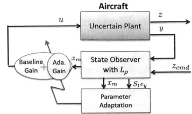
4-1 The architecture of the adaptive output-feedback controller: an adap-tive component is added to a baseline observer-based controller . . . 51

4-2 The Bode plot of the SPR system

{(A

C}

VFA model using the SPR/LTR observer parameter L = L, 67

4-3 L, in the baseline controller is able to recover the phase condition of

{(A+

- LPC), B, SC}

*

4-4 The Nyquist plot of the loop gain at input, La(s), of the baseline controllers, compared with that of the LQR controller for the 3-wing V FA m odel . . . . 67

4-5 The simulation results of the vertical acceleration tracking of the 3-wing VFA using the adaptive output-feedback controller, compared with the baseline SPR/LTR controller . . . . 69

4-6 The "snapshots" of the closed-loop systems for the 3-wing VFA model in the simulation shown in Figure 4-5b . . . . 70

4-7 Comparison of the maximum and minimum singular values of the transfer function matrix between the original Vulture VFA model and the reduced-order model . . . . 71

4-8 The zoom-in map of poles and transmission zeros of

{(A-LPC),

SC}

4-9 The frequency domain analysis of the closed-loop system using the baseline SPR/LTR controller on the Vulture VFA model, compared

with a LQ R . . . . ...72

4-10 The flight path and flexible wing shape of the Vulture VFA in the BTT

maneuver, controlled by the adaptive SPR/LTR controller. . . . . . 74

4-11 The tracking of roll angle ($) and side-slip angle (3) in the BTT

ma-neuver of the Vulture VFA through thrust (T) and tail (J1) using the

adaptive controller, compared with the baseline controller and a LQR. 75

4-12 The adapted parameters settle down to steady-state values after three

step commands of BTT for the Vulture VFA . . . . 76

5-1 The tracking of q and A, using the relative degree two adaptive

con-troller for the nonlinear 3-wing VFA model . . . . 90

5-2 The parameter trajectories of the relative degree two adaptive

con-troller in the simulation shown in Figure 5-1b for the nonlinear 3-wing

V FA m odel . . . . 91

5-3 The frequency domain analysis of the snapshot closed-loop system

shows that adaptation mitigates the effects of model uncertainties on the robustness of the "snapshot" closed-loop systems for the 3-wing

V FA m odel . . . . 91

6-1 The tracking of 71 and A. using the relative degree three adaptive

con-troller on the nonlinear VFA model . . . . 123

6-2 The parameter trajectories of the relative degree three adaptive

con-troller in the simulation shown in Figure 6-1b for the nonlinear 3-wing

VFA m odel . . . . 124

6-3 The spectrum of the aileron Ja response in the simulation shown in

Figure 6-1b for the nonlinear 3-wing VFA model . . . . 124

6-4 The frequency response of the snapshot closed-loop system with the

relative degree three adaptive controller, from J, to V, and the effects

6-5 The frequency domain analysis of the snapshot closed-loop system shows that adaptation mitigates the effects of model uncertainties on

robustness for the 3-wing VFA model . . . . 125

6-6 The time domain response of q and Ja when subject to sinusoidal

dis-turbance/noise of magnitude 0.2 and frequencies 0.3, 2, 3 rad/sec for

the nonlinear 3-wing VFA model . . . . 127

6-7 The mean of the moving window standard deviation (MMSTD) of 7

tracking and 6, control when subject to sinusoidal disturbance/noise

List of Tables

Chapter 1

Introduction

1.1

Large Dimension MIMO Systems

To achieve engineering marvels, modern machines are made of a huge number of intricate components and mechanism, and therefore include complicated dynamics. Control designs that are based on a simplified low-order plant model cannot produce stable performance in all operation range while applied on the real machine, while control designs based on high-fidelity high-order models usually yield a much higher order controller that defies efficient implementation. These large dimension systems are also equipped with a large number of sensors and actuators, and are required to perform a complex maneuver that involve all sensors and actuators simultane-ously, which defies classical single-input-single-output (SISO) decoupling approach and therefore motivates a MIMO approach. One of such large dimension MIMO control challenge is Very Flexible Aircraft (VFA) [1, 2].

1.2

Very Flexible Aircraft

VFA platforms are being investigated with increased attention in the last decade, motivated to a large extent by the desire to generate high-altitude long-endurance

(HALE) flights [1, 3,4]. VFA corresponds to an aerial platform whose equilibrium

of the challenges of VFA is a significant change in the rigid-body dynamics around a trim as its wing morphs. For example, the pitch (short period) mode of VFA

can become unstable when wing dihedral is trimmed at a high value [5,

6].

consequence, control designs based on low-order rigid-body dynamics only may face unexpected adversities. An example of this adversity occurred in 2003 during the second test flight of Helios when the flight controller failed to regulate the wing dihedral and eventually, allowed the unstable pitch mode to diverge [6]. The lesson learned from the mishap is that the model for control designs has to include body

flexible effects [5,6].

Nonlinear VFA models have been investigated in [5,7,8] with focus on capturing the flexibility effects while VFA navigates through multiple trims. For maneuvers around a single trim, high-fidelity linear model, such as the one for Vulture VFA [2], is also introduced with the focus on verification of the control design for large dimension systems. All these platforms feature a particular challenge that only a set of state measurements can be used for control because body flexible modes have to be included in the model but none of them are measurable. The restriction necessitates control designs based on output-feedback, such as linear observer-based controllers.

1.3

Linear Output-Feedback Control

Output-feedback MIMO control designs have been studied extensively because of their ability to control a plant with only incomplete state measurements. One strat-egy is to use an observer to generate state estimates, and use the estimates to perform state-feedback-like control [9]. Observer-based controllers have been widely employed for aircraft control and their performance is quite satisfactory for a nominal lin-ear time invariant (LTI) plant model, which are able to capture most of the rigid body dynamics [10,111. Combined with the "full-state" loop transfer recovery (LTR) technique [9,12] (referred as the LTR technique hereafter), the resulting controllers, denoted as observer-based LTR, recover the guaranteed stability margins of linear

certain amount of model uncertainties. Application of observer-based LTR controllers to VFA, however, faces unique difficulties. First, since flexible wings can deform to an unknown shape, the actual trim and the corresponding flight dynamics can drift far away from the nominal trim and its nominal dynamics (trim drift). Second, a HALE flight can cause severe actuator anomalies such as power surge in motors or structure damage on control surfaces. Both unknown adversities can exceed stability margins of observer-based LTR controllers, and therefore make these controllers inadequate

for VFA.

1.4

Adaptive Output-Feedback Control

The limitations of linear controllers motivate an adaptive control solution that is able to accommodate the unknowns associated with VFA flights. Those unknowns include unknown structure stiffness and compliance change caused by unknown trim drift, which is another consequence of unmeasurable states, and unknown scaling of lift/thrust force caused by actuator anomalies. This thesis will show that both types of the unknown adversities can be modeled as parametric uncertainties in the underlying plant model.

For uncertain plant models, adaptive control has been investigated as a candi-date improvement over linear controllers for the reason that it guarantees to recover both stability and performance despite the presence of large parametric uncertain-ties [14]. The classical approach to MIMO adaptive controllers (see [14, Chapter 10]

and [15, Chapter 91) is based on the underlying plant transfer function matrix. Such

a design typically requires the knowledge of plant's Hermite form [16,171 and uses a non-minimal observer along with a reference model, resulting in a significant num-ber of integrators (a high order controller). These high order designs prohibit their applications to VFA since VFA model usually features large amount of flexible states.

1.5

Relative Degree One Observer-Based Control

De-sign

In contrast to the classical method, recent literature proposes a new approach of adaptive control based on state-space representation, which uses a minimal observer to generate the underlying state estimates [18, Chapter 14]. The state estimates are then used for both feedback (similar to observer-based linear controllers) and parameter adaptation. Unlike the classical approach, the observer is also used as a reference model, by appealing to the notion of a closed-loop reference model (CRM), which is recently shown to be a highly promising direction in adaptive control due to improved transients [19-21]. The presence of CRM allows the new controllers to use much fewer integrators than the classical ones, and is therefore an attractive alternative in the case of MIMO plant models (see [18,22-24]). The proposed controllers in these references guarantee stable adaptation based on an underlying strict positive real (SPR) condition and therefore can be applied on a plant model with relative degree one. Implementation of the proposed controllers requires solutions for its parameters, which are subject to a matrix inequality, and therefore are solved using numerical methods in these references. As a result, applications to a large dimension plant model, or analysis of LTR properties, are not available.

1.6

Higher Relative Degree Control Design

The adaptive controllers proposed in the above-mentioned references [18,23-25] are based on a restrictive assumption that the underlying relative degree of the plant is unity. This implies that any actuator dynamics that may be present has to be sufficiently fast, and also that the set of sensors must result in the number of net integrations to not exceed one (for example, velocity sensors for mechanical systems). Since actuator dynamics or sensor dynamics are hardly negligible in real applications, especially for HALE flight where actuator/sensor aging could take place, high relative degree plant models with uncertainties in both the plant dynamics and the

actua-tor/sensor dynamics need to be considered. While adaptive controllers for such kind of plant models have been addressed in SISO plants [21], currently very few results exist for this case in MIMO plants. Classical adaptive control approach (see [14, Chap-ter 10] and [15, ChapChap-ter 9]) addresses MIMO plant models with high relative degree at the cost of huge amount of integrators and therefore are not suitable for large dimension systems such as VFA applications.

1.7

Nonsquare Plant Models

Square systems play a key role in control theory development because of some unique properties they may possess such as SPR properties [26], which serves a crucial role in guaranteeing stability. Therefore, in adaptation design for MIMO plant mod-els [14,15], square plant modmod-els with stable transmission zeros are commonly as-sumed. Nonsquare plant models, whose number of outputs exceeds number of inputs, become increasingly popular in industry since sensors are cheap and can be massively deployed. The fact that nonsquare plant models usually do not have transmission ze-ros makes them a good candidates for adaptive control design. To extend control de-sign to non-square systems, a squaring-up method is usually needed, which effectively produces an artificial square system through addition suitable inputs. Literature on squaring-up methods were rather sparse until the work by [27,28]. The squaring-up method in these references, however, are subject to a restrictive assumption that the underlying plant models have uniform relative degree one, which prevents the design to be applicable to plants that have actuator dynamics, i.e. higher relative degree.

1.8

Synopsis of Thesis

The main contribution of the thesis is the development of an adaptive output-feedback controller for a class of MIMO plant models with unequal number of inputs and out-puts and arbitrary relative degree, and the demonstration of the design on a high-fidelity large dimension VFA model for high-altitude flight with body flexible effects.

First, a generic class of MIMO plant models that are suitable for control purpose, in particular for VFA control, is examined in Chapter 2. Then mathematical prelimi-naries necessary for control design and analysis are introduced in Chapter 3. While assuming no actuator dynamics present, we develop an adaptive controller for the plant model with relative degree one in Chapter 4. In Chapter 5, we then explicitly consider actuator dynamics and extend the control design to plant models with rel-ative degree two. The control design is further extended to relrel-ative degree three in Chapter 6, which serves as a corner stone to extend the whole design to arbitrary

relative degree in Chapter 7. Squaring-up method are provided in each section such

that the overall method can be applied on nonsquare plant models. Simulations with high-fidelity VFA model are presented at the last section of each chapter for each of the control designs. All proof of the Propositions, Lemma, Theorem can be found in the Appendix.

1.9

Thesis Contributions by Chapter

The main contributions of the thesis is described in Section 1.8. The following para-graphs are thesis contributions by chapter.

Chapter 2

A class of nonlinear VFA model as proposed in [81 is properly linearized and is shown

to contain parametric uncertainties due to unmeasurable flexible effects. This class of linearized VFA model is shown to belong to a generic class of MIMO plant models.

Chapter 3

Based on a series of definitions and properties pertain to relative degree

[29,30],

Chapter 4

Based on the previous adaptive control design for relative degree one plant models

[18], a new explicit closed-form solution for its parameters is proposed and shown

to guarantee an underlying SPR condition while retaining the LTR properties in the baseline controller. The design is also extended to plant models with nonlinear parametric uncertainties. Demonstration of the control design on a large-dimension nonsquare VFA model is carried out around a single trim.

Chapter 5

Using a recursive property of the new control parameter design, the relative degree one adaptive control design is extended to plant models with relative degree two. Extension to nonsquare plant models whose number of outputs exceeding number of inputs is also integrated into the design. Demonstration of the control design on a nonlinear VFA model is carried out while the VFA navigating through multiple trim.

Chapter 6

The relative degree two adaptive control design is extended to nonsquare plant models with relative degree three. Demonstration of the control design on a VFA model ver-ifies that significantly less number of integrators are used compared with the classical adaptive controllers.

Chapter 7

The adaptive control design is extended to nonsquare plant models with arbitrary relative degree.

Chapter 2

Plant Model Description

This section describes a class of MIMO plant models that are commonly seen in real world applications. First a generic class of uncertain MIMO plant models is examined in Section 2.1. The main focus of this thesis is presented in Section 2.2, where a class of VFA model is examined and shown to be a MIMO plant model with parametric uncertainties. Then Section 2.2.1 presents a 3-Wing VFA model that belongs to the class and will be used for our simulation validation. Section 2.2.2 describes another example of the class, the Vulture VFA model, that will be used for the verification of the design on a large dimension plant model.

2.1

A Class of Uncertain MIMO Plant Model

Dynamics of a MIMO plant around an equilibrium flight condition can be described

by a linear time invariant (LTI) model as

x= Ax + Bu

(2.1)

y = Cx

where x E R' are states, u E R" are control inputs, and y E RP are measurement outputs. A E R"X", B E Rnm, C E RPXf are known matrices which represent a nominal model. Since in most flight control applications, there are more sensors than actuators (as sensors are much cheaper than actuators), and all states are not

measurable, we assume that n > p > m.

Eq.(2.1) corresponds to the ideal case where all plant matrices are known. In

reality, these matrices are unknown and are identified through various methods. The state matrix A can be determined through experiments fairly accurately, such as wind-tunnel tests for aircraft frame. C is well known as well since the relation between measured outputs and states is well defined. The input matrix B, in contrast, may not be accurate as the net effect of control inputs are subjected to perturbations. We address two of the dominant issues in this section.

The first source of uncertain perturbations we consider is the unknown structural stiffness, compliance or weight distribution change. In most cases, this effect can be modeled as an additive term 0*T<D(x) where <D(.) : R' -+ R' is a known nonlinear function regressor and

e*

source of uncertainties that we consider is actuator anomalies caused by electronic power surge or control surface damage. This is modeled as an unknown multiplicative factor A* E Rmxm. Together, both uncertainties lead to a modified plant model given

by

= Ax + BE*T<(x) + BA*u (2.2)

y = Cx

The class of plant model as in (2.2) is generic and can model a variety of real dy-namics. For example, it can model the response of vertical acceleration of aircraft when elevators move, in which case E* are the uncertainties in the CG position of the aircraft [18, Chapter 21. Another example is the response of pitch/roll/yaw angles of a quadrotor when some of its motors change power output, which is summarized below.

Example 2.1.

[31]The

orientation can be described by a linear model that belongs to (2.2) as

i=go, j=-gop,

=(U1+ AU)

S ++(2.3)

where variables w, y, z are the positions of CG in the inertial frame; Variables <), 0,

'

by the four rotors, and AU1, AU2, AU3, AU4 are their associated uncertainties caused

by motor/propeller deficiency.

Another example is the response of cart position when the mounted inverted pendulum is pushed, as summarized below.

Example 2.2. The dynamics of cart position around the unstable equilibrium 0 = 0, po = 0, where 0 is the angle between the bar and the vertical line, p is the horizontal

displacement of the cart, belongs to the class of (2.2) and can be written as

0 1 0 0 p 0 0 00 g 0 P M M 0 0 0 1 0 0 0 0 0 g(M+m) 0 # (2.4) A x B y =[P]= 1 0 0 0 1X C

where u is the force input and

e*

In all the cases discussed above, <D(x) can be as simple as x, and A* are the uncertainties in the control effectiveness due to motor or control surface damage. Detail assumptions on the class of plant models (2.2) will be discussed in the beginning of each control design section. Among these assumptions, the relative degree of the plant model is the major topic of this thesis.

2.2

VFA Model

This section will show that a generic VFA model, if linearized around a trim, also belongs to the class of MIMO plant models presented in (2.2). Our starting point is a nonlinear VFA model including its complete rigid body dynamics and flexible component dynamics, which is derived in [8I using the virtual work method as

MFF MFB

1FF

1

MBF MBB

]

J

+

=

0

0

b

assuming:

Assumption 2.1. The coupling between rigid body and flexible elements are caused

by inertia and compliance property change only;

Assumption 2.2. Control surfaces span the entire wing;

Assumption 2.3. Properties of aircraft vary slowly with respect to the rigid body position and orientation;

Assumption 2.4. External loads weakly depend on body acceleration;

Assumptions 2.1 and 2.4 implies that aerodynamic coupling is negligible. e are states of the flexible wing with elements being states of each discretized flexible seg-ments, and b =

#

#

$and

Jhb(e, b) = SL as the Jacobian matrices with h(e, b) being the lumped coordinate

transformation effects integrated along wing span. Since h, = 92 + -2Lb and

specifically,

MFF(e) = JhMeJhe, MBF(c) = JhbMeJhe

MFB(E)= JhMeJhb, MBB(E) =J7MeJhb + MRB

CFF(E, ,73) = Jh MeJhc + Ce, CBF(E, ,# ) = JhiMeJhe (2.6)

CFB(E, 0,) = J Me B Jhb + 2JMe jhb

CBB(E, ,0) fbMeQBJhb+ 2JhbMejhb+ CRB

BF(E) = Jhe, BB(E) = Jhb,

where M(.) is the effective inertia, C(.) is the effective compliance, Fload( e, E, 03, /, uS)

is the aerodynamic load (see

181

compliance matrices C(,)(.) are only functions of c, ,

/3.

loading Fload are calculated locally at wing segments and then summed along the

wing span. It is noted that because inertia, compliance and external load effects are all subject to local coordinate transformation, M(.)(-), C(.)(.) and B(.) all have Jhb or

Jh, as their leading factors.

To design a controller for a trim [Eo, o, Eo, )o, ouo]T, we first define deviation

states and inputs as x= - - - 0]T E Rn and up = (us - uo)

c

respectively, and perform model linearization (ignoring high-order error terms), which generally leads to a linear parameter varying (LPV) plant as

Q1.4

where

Q,

both are functions of (do, o, o, 1%, #o) (see

181

Q3

introduces model uncertainties as

Qi =

Q(0,

0, eo,,!o) +

AQ(o, ,/3o)

Q1 -UO71607700

Q2=Q ₂

(0,0,o,0,#0)+AQ(Eooo).

(.

where Q₁ and

Q

Q3,

are the unknown to the controller. Eq.(2.8) transforms the plant (2.7) into a special form as specified in Lemma 2.1, whose proof can be found in Appendix A.

Lemma 2.1. The nonlinear VFA model (2.5)(2.6) that satisfies Assumptions 2.1 to

2.4, has the unknown AQ* and AQ* that can be parametrized as

AQ*

=

Q

*7(2

,

,3

), AQ(*

Q

e*(j

,

,

!O),

(2.9)

and the model can be linearized around an unknown trim (O , eo, 60, /37, 11uo),

produc-ing an uncertain LPV plant as

= (AP + BPE;*T)xp

+

P P P(2.10)

yp = Cpxp

where AP(e0, b, uO) = Q Q2 Bp(c0, f00, UO) = Q3 are known plant parameters,

while =* q*T 9q,- Ap

--q

+

Q

Q3)

*T, and

A* = A*, where A* = (I - * Bp), are unknown.

Eq. (2.9) implies that the local body inertia and compliance changes caused by local

wing deformation can be approximated by similar changes caused by external loads.

In realistic applications, A* can include control effectiveness loss A* as A* = A*A*

where A* can be present due to possible control surface damage. Eq.(2.10) is the actual uncertain LPV plant model when aircraft flies through different trims. If we assume that

Assumption 2.5. All aircraft properties vary slowly around a trim,

then all matrices in Eq.(2.10) are constant and Eq.(2.5 becomes a linear time invariant model, which belongs to the class of plant models in (2.2). The following

two subsections present two VFA model examples that belong to the generic VFA model class (2.10).

2.2.1

3-Wing VFA Model

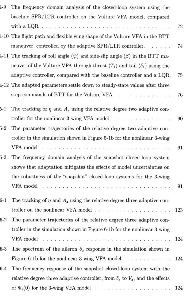
Consider a simple VFA comprised of three rigid wings with elastic pivot connections adjoining them [5]. The longitudinal and vertical dynamics of the 3-wing VFA is coupled with the dynamics of rotational movement of outer wings with respect to the center wing about the chord axis, as shown in Figure 2-1. The angle between the two wing planes is denoted as wing dihedral (,q).

Figure 2-1: The illustration of 3-Wing VFA

The platform captures essential flexible wing effects and can be viewed as building blocks of large VFA. A 6-state nonlinear model has been developed in [5, Eq.s (45) and (46)] including aircraft's pitch mode and dihedral dynamics. Define V as airspeed, a as the angle of attack, 0 as pitch angle and q as pitch rate. The nonlinear model can be rewritten in the form of (2.5) with e = r and 3 = [V, c, q]T:

d3(7) sacq 0 0 - -_c_ _k s17 cqca 0 17sca 7

0 m 0 0 + 0 0 0 g V 0 0 mV 0

L

where s(-) = sin(.), c(.) = cos(-) and 6, and 6a are properly scaled. Parameter ci

and c2 are inertia constants that depends on aircraft physical properties, and d3(7) is the rotation inertia about longitudinal axis and therefore a function of q (see [51).

Measurements are vehicle vertical acceleration A2, r and q. Other states, a and i/,

are unmeasurable and are unavailable for control. The nonlinear model was trimmed at 30ft/sec airspeed, 40,000 ft altitude and different dihedrals, and the corresponding

linearized models with respect to each dihedral were obtained

15]

be written as V -0.279 3.476 -32.2 -0.015 0.514 0.525 V -2.57 -6.47 a -0.070 -4.104 0 1.013 0.193 0.100 a -0.795 -0.079 9 0 0 0 1 0 0 8 0 0

[

[

~I

where three aileron are bundled as one control 6

a and three elevators are bundled as

one control 6e. The pitch mode is stable for this trim. Local stability analysis shows that when the dihedral is above 15', the pitch mode becomes unstable [5]. Let's consider the uncertainties that may exist in the plant model. First, there might be a control surface damage that reduces control effectiveness to 10% (A* = 0.1). Second,

since the outer elevators are connected to the outer wings, their control effectiveness is locally linearly proportional to q and therefore is a function of

e*x

of uncertainties, we obtained the linearized model for 71 = 160 and 2 = 0.2 deg/sec, which can be parametrized with in the form of (2.12) with (Ap, Bp, Cp) for 27 = 10'

and 6 = 0 deg/sec, and

A* = 0.1;

T=

[

0.02 -31.94

0.12 0.91 9.1 -9.28

(2.13)

2.2.2

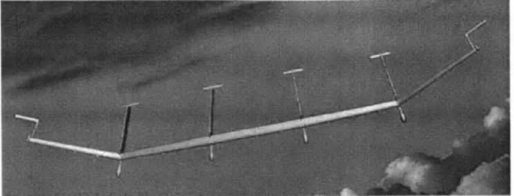
Vulture VFA Model

Recently, a large VFA platform, denoted as Vulture, has been under development to meet the goals of HALE maneuvers. Vulture is an experimental aircraft with a wingspan of 400ft. Its entire wing is made of light low-yield material and is flexible to deform. 3-wing VFA example shown in the previous subsection represents building blocks of the Vulture VFA. One can consider the wings of the Vulture as hundreds of 3-wing segments adjoined together. The huge wings are in junction with 4 long booms in the middle of wingspan and 2 end devices at the tips, as shown in Figure 2-2.

Figure 2-2: The illustration of Vulture VFA

A large dimension model has been developed for Vulture with 707 states, 21

control inputs and 212 outputs, representing the VFA trim at a nominal HALE flight condition at a cruise speed of 34.6 ft/sec, an altitude of 66,000 ft, and with zero dihedral [2]. The 21 inputs includes 15 engine propellers evenly placed across the wingspan and 6 tail elevators at the end of each boom (see Ref. [2] for details). If dividing the 707 states into three groups, i.e. 12 rigid body dynamics states XRB for

6 vehicle degrees of freedom, 340 flexible positions xf ex, and 340 flexible velocities

Vflex, the Vulture model manifests itself in the following block matrix form:

[

H

[

Iex 0 0 I xf lex + 0 Up+ 0 n + 0 6i

Vflex x x o\o vflex x x

P AP XP Bp

yP = x 0 0

x + DPUP + Din, +

(2.14)

where x represents dense entries, * represents sparse entries and o\o represents di-agonal entries. Some observations are made. First, the flexible modes are strongly coupled with rigid-body dynamics. Second, the control u only acts on flexible

com-ponent. Third, there are control rate

Q,

represent aero-elastic-coupling between unsteady aerodynamics and flexible effects of boom. These features imposes great control challenges. For the control design, we

will pretend that the itp and ii, terms are not present and therefore the resulting

(2.10). For the actual simulation we will bring back the it, and fi, terms (called the evaluation model).

Chapter 3

Preliminaries

This section presents definitions and lemma that will be used to handle high relative degree systems. Proofs of all results in this section are redirected to the corresponding references. First we define index notations in superscript and subscript that are often used in a zero polynomial.

Definition 3.1. No bracket is number of power operation, i.e.xf+l - X{n+1} n .

[ bracket is index for variable notation, for example,x[ 2+11 X[31; and () bracket is

the number of derivative, for example X(2)

-Define s as the differentiation operator, i.e. st[-3 = [_] = [_](i), and define 7r (s)

as what follows.

Definition 3.2. Define 7r'(s) as a ith order polynomial in s with a" as the its

coeffi-cients, i.e.

7r'(s) = (s + aC 1)(s + a2) ... (s + aj) = a-si-j (3.1)

j=0

for i = 1, 2, ... , r, and ai E C; Define d. as the coefficients of differentiation operation,

i.e. sr(xy) = drx(r)y + drlX(r-1)y(1) + - + dxy(r).

Remark 3.1. In particular, s(-1)[] = f[-]dt. 7rr(s) arrange coefficients in a reverse way (for example, iro(s) = a2, 7r'(s) = a s + a' and r 2(s) = a s2 _{+ a's + ao)}

so that

irk(s) . Sr~ + a csi = ir+1(s) (3.2) j=0

has a recursive property.

Consider a state space representation

{A,

Square systems have m = p while nonsquare systems have m 5 p. The notation

{A, B, C, D} is defined as the transfer function matrix G(s) = C(sI - A)- 1B + D.

The case when D = 0 is denoted as

{A,

follows.

Definition 3.3. If for an m-input p-output linear system G(s) = C(sI- A)--1 B+D,

the rank of G(s) is strictly less than min(m, p) for any s E C, where C is the set of complex number, then the system is degenerate.

Most real linear plant models are non-degenerate, whose transmission zeros can be defined as follows.

Definition 3.4. [33] For a non-degenerate m-input and p-output linear system with

minimal realization A E R'X"n, B E R"x" , C E RPXn and D E RPxm, the transmission zeros are defined as the finite values of z such that rank[R(s)] < n + min[m, p], where

zI -A B

R(s) =

.

C D

Transmission zeros represent a state trajectory that cannot be detected by any of the outputs. Most non-square linear systems don't have transmission zeros; square systems are more likely to lose rank and therefore more likely to have transmission zeros [34]. Generally, for MIMO plants transmission zeros and individual transfer function zeros are different. An example below illustrates the difference.

Example 3.1. In Example 2.2, the SISO plant model

{A,

g, M ,

" , - (M"m) and two zeros at a, -

V.

mea-0, mea-0, Ml') I l ' VL'

surement of the tilt angle rate 0 is included in y as

y 0 x. (3.4)

Then the resulting single-input-multiple-output does not have any transmission zeros. However, choosing an additional mixing measurement as

p 10 0 0

y 1 (3.5)

- + + P 1 0 1

-results in a plant model with a transmission zeros at . The ratio of mixing has to

be exact for the transmission zero to exist.

We part B into columns as B =

[

the ith input ui. The input relative degree of the plant model is defined as following.

Definition 3.5. A linear square plant model {A, B, C} has

]T

a) input relative degree t = rl r2, - , rm E Nxi if and only if

i) Vi E {1, m}, Vk E 10, .-- rj - 2}1

CAk bj = Omxi, and (3.6)

ii) rank I CAr-b1 CAr2-1b2 ... CArmlbm =m; (3.7)

b) uniform input relative degree r E N if and only if it has input relative degree

r ri, r2, --- ,rm Iwith r = r1 = r2 =---=rm.

Remark 3.2. If {A, B, C} has ui of input relative degree ri, one needs to differentiate ui rith time to make'ui shows up in the y equation, i.e.

C(sI - A)1 bi - s = C(sI - A)-1Abi

(3.8)

C(sI - A)-Sbi- = C(sI - A)-'A- 1

C(sI - A)lbi. sri =C(sI - A)--1 Abi + CAri-lbi

where we have used Definition 3.5 and the identity (sI - A) 1 s = I + (sI - A)1 A..

The term "relative degree" is referred to input relative degree in this paper.

and ii) are generically satisfied. The input relative degree relates to the transmission zeros of the plant model in the following Lemma (see [35, Corollary 2.6] for proof).

Lemma 3.1. For a square system { A, B, C} with uniform input relative degree r,

define

C

C

A-CA=, 93:=[B

C Ar-1

with C E R" m , (E RE x"" Y

9A

(EM = 0, and

9 = (TIT9R) -l9JT[In - ( E (n-mr)xn (3.10)

such that 919 = 0 and 91 = 1nmr. Then C93 is full rank, and the eigenvalues of

Z

XA931

are the transmission zeros of the { A, B, C}.

Lemma 3.1 can be directly extended to the plant model with nonuniform relative degree. It follows Lemma 3.1 that the number of transmission zeros are related to the relative degree in the following way (see

135]

Corollary 3.1. The number of transmission zeros nz of a plant model with relative

T

degree r

[

nz = n - r. (3.12)

where r, = ri and n is the number of states.

Realization of a transfer function matrix is not unique. Two realizations of linear time invariant systems are equivalent if they share a same transfer function. A spe-cial state space realization, called "input normal form", will be used to write system

matrices with respect to its relative degree, as stated in the Following Lemma, whose proof can be found in [35, Theorem 2.41.

Lemma 3.2. [Input Normal Form] For plant models {A, B, C} with uniform relative

degree r, there exists an invertible coordinate transformation matrix

Tin = Ti-n D (3.13)

where 9N and It are defined in Lemma 3.1, that can transform the plant model into

0

0

R

2 Im --- 0 R₂ 0 0

:0 + : u

&

S0 -

0

Ain xin Bin

y

=

Cin

using xin = Tinx, Ain = TnAT-;n , B = TinB, and C = CT;, where Z C

R(n-3m)x(n-3m) has eigenvalues that are transmission zeros of

{

{A, B, C} and {Ain, Bin, Cin} are two equivalent realizations. Systems with differ-entiator s added to inputs also have equivalent realizations, as stated in the following Lemma, whose proof can be found in the Appendix B.

Lemma 3.3. Given a linear system

{A,

i)

= Ax + B7rr-i(s)[u](.

r-1 _(3.15)

y = Cx

ii)

= Ax' + B'u

r _(3.16)

y = Cx'

where

B

Z=

A'- Ba-I-j = 7r- (A)B.

(3.17)

j=0 and x' is a new state coordinate.

Remark 3.3. It is noted {A, Br, C} has relative degree i, and as a result, we name B' as "the input path with relative degree i". It is noted that the implementation

of representation (3.15) usually requires differentiating input u first and therefore is not feasible, while the implementation of (3.16) does not require differentiating u first and is generally feasible. For this reason, we will design controllers using (3.16), and will use (3.15) for analysis. Two state coordinates are related as

r

x

-

E (B si--)[u].

(3.18)

j=i+1

(3.15) differentiates inputs of a relative degree r system

{A,

which adds (r - i) transmission zeros to {A, B, C}, as stated in the following

propo-sition, whose proof can be found in the B.

Proposition 3.1. Define Z{} as the set of transmission zeros of transfer function

{}

then

Z{A, Br, C}

=

Z{A, B, C}

Z[7r2 _-(s)]

One special category of plant models with relative degree is the relative degree one plant models. Relative degree one plant models have the following property, which is a special case of Lemma 3.1 (see Ref.

[29]

Corollary 3.2.

[291

{A,

NB = 0(n._)xm, CM = 0mx(nm), NM = I(nm)x(nm) and the eigenvalues of (NAM) are the transmission zeros of { A, B, C}.

One special category of relative degree one transfer functions is a strictly positive

real (SPR) transfer function. This thesis uses Ref. [14, Definition 2.10] for the defini-tion of SPR. Kalman-Yakubovich-Popov (KYP) lemma links the frequency domain properties of an SPR transfer function to its realization.

Lemma 3.4. [KYP Lemma! A system { A, B, C} is strictly positive real if and only

if there exists a P = PT > 0 such that

PA + ATP < 0 (3.19)

PB = CT. (3.20)

An SPR {A, B, C} is a square system satisfying CB = BTPB = (CB)T > 0.

With the definition of N, Eq.(3.20) of KYP Lemma can be fully characterized as following (see Ref. [36] for the proof).

Lemma 3.5. [36J Given a pair of B and C, if there exists a P = pT > 0 such that

PB = CT , then P E Y where

= {P > 0 | P = CT(CB) 1 C + NTWpN, W, > 0}, (3.21)

N is the right null space of B and W is an arbitrary symmetric positive definite

matrix.

Lemma 3.5 implies that given a pair of B and C such that CB = (CB)T > 0, a P > 0 that satisfies PB = CT can be calculated using (3.21). From Lemma 3.2, it can be concluded that having stable transmission zeros is a necessary condition for

the system to be SPR. This can be shown by pre and post-multiplying Eq. (3.19) with

MT and M, respectively, and appealing to Eq.(3.21), which yields

For Eq.(3.22) to hold for an symmetric positive definite (SPD) W,, NAM has to be Hurwitz.

Another special category of plant models with relative degree is the relative degree

zero plant models {A, B, C, D}. Relative degree zero plant model can also have

SPR properties. The following states the multivariable case of Lefschetz-Kalman-Yakubovich (LKY) Lemma regarding to SPR relative degree zero plant models.

Lemma 3.6. [26,37, 38]Assume (A, B, C, D) is a minimal realization of G(s); Then

G(s) is SPR if and only if a 'y > 0, a matrix P = PT > 0, a matrix L > 0, and

matrices W and K exist such that

PA+ ATP = -WTW - L (3.23)

PB = CT +.WT K (3.24)

KTK = D + DT (3.25)

Lemma 3.4 and Lemma 3.6 leads to a Corollary that states the close relation between a SPR relative degree one plant model and a SPR relative degree zero plant model.

Corollary 3.3. If a transfer function matrix { A, B, C} is SPR, then there exists a

a* > 0 such that the transfer function matrix { A, B', C, aCB}, where BO = aAB

+

is SPR for all a < *; and {A, B, C} and { A, BO, C, aCB} share a same P = pT > 0

that satisfies the results of Lemma 3.4 and the results of Lemma 3.6, respectively.

The following proposition provides formulation of parameter errors in the presence

of s, which will be used in parameter adaptation design and error model formulation.

The proof is rather straight forward and therefore is omitted here.

Proposition 3.2. Suppose s is the differentiation operator,

#*T

where qT(t) := cT(t) - $*T , and 7r'(s) is defined in (3.1)

for

The 2 _{1, Y2 and Y,, bound of a time series signal x(t) is defined in}

_114,

Chapter 4

Relative Degree One Design

This section presents the adaptive control design for relative degree one plant models, and is organized as follows. Section 4.1 formulates the control problem in the context of VFA. Section 4.2 presents the adaptive controller design and its SPR/LTR prop-erties, and also includes stability analysis of the adaptive system. Section 4.3 demon-strates the response of the resulting closed-loop system with the adaptive controller using two numerical examples, including the 3-wing VFA model and the Vulture VFA model [21 around a single flight condition.

4.1

Relative Degree One Problem Statement

Following the description in Chapter 2, an application-driven nominal plant model with relative degree one is described as

x, = Apxp + Bpu

yP = CPxP (4.1)

z = C,2x, + Dp2u

where xP E R" are states, uP E R' are control inputs, and y, E RPP are measurement

outputs. In addition, tracking outputs z E Rd are also measured. An example

of z is the vertical acceleration measurement in aircraft. We assume np > pp and

accelerations, a constant matrix Dp, is assumed to be present. If in some cases, y, includes non-strictly proper outputs, they are integrated to become strictly proper

outputs. C, E Rdxnp and D,

c

While Eq.(4.1) represents a nominal plant model, the actual plant model consid-ered in this section is written as

4= AXP + BA*[u +

*T

D(x)]

yp

z = _{CZzX + DpzA*[u}

₊

where

e*T4b(xp)

E*T

E*.

The adaptive controller that we will present in this section requires the following assumptions regarding the plant model in (4.2):

Assumption 4.1. (Ap, Bp) is controllable and (Ap, Cp) is observable;

Assumption 4.2. { A,, Bp, Cp} has stable transmissions;

Assumption 4.3. {Ap, Bp, Cpz, Dpz} does not have a transmission zero at the origin;

Assumption 4.4. rank(CpBp) = m.

Assumption 4.5. A* is diagonal, full rank, bounded by a known value,

I|A*||

and the sign of each element sign(A*) is known;

Assumption 4.6.

e*