Advanced prognosis and health management of aircraft and spacecraft subsystems

Advanced Prognosis and Health Management of

Aircraft and Spacecraft Subsystems

by

Heemin Yi Yang

S.B.E.E.C.S., Massachusetts Institute of Technology (1998)

Submitted to the Department of Electrical Engineering and

Computer Science

in partial fulfillment of the requirements for the degree of

Master of Engineering in Electrical Engineering and Computer

Science

at the

MASSACHUSETTS INSTITUTE OF TECHNOLOGY

February 2000

©

Heemin Yi Yang, MM. All rights reserved.

The author hereby grants to MIT permission to reproduce and

distribute publicly paper and electronic copies of this thesis

document in whole or in part. MASSACHUSETTSINSTITUTE

OF TECHNOLOGY

A

JUL

3 0 2003

LIBRARIES

A uthor ...

...

DeDartment of E

ineering and Computer Science

Fpbruary 3, 2000

BARKER

Certified

_....

.-David H. Staelin

Professor of Electrical Engineering

Thesis Supervisor

Accepted by ....

Advanced Prognosis and Health Management of Aircraft and

Spacecraft Subsystems

by

Heemin Yi Yang

Submitted to the Department of Electrical Engineering and Computer Science on February 3, 2000, in partial fulfillment of the

requirements for the degree of

Master of Engineering in Electrical Engineering and Computer Science

Abstract

Beacon Exception Analysis for Maintenance (BEAM) has the potential to be an efficient and effective model in detection and diagnosis of nominal and anomalous activity in both spacecraft and aircraft systems. The main goals of BEAM are to classify events from abstract metrics, reduce the telemetry requirements during nor-mal and abnornor-mal flight operations, and to detect and diagnose major system-wide changes. This thesis explores the mathematical foundations behind the BEAM pro-cess and analyzes its performance on an experimental dataset. Furthermore, BEAM's performance is compared to analysis done with principal component transforms. Met-rics are established where accurate reduction of observable telemetry and detection of system-wide activities are stressed. Experiments show that BEAM is able to de-tect critical and yet subtle changes in system performance while principal component analysis proves to lack the sensitivity and at the same time requires more computa-tion and subjective user inputs. More importantly, BEAM can be implemented as a real-time process in a more efficient manner.

Thesis Supervisor: David H. Staelin Title: Professor of Electrical Engineering

Contents

1 Introduction ₁₁

1.1 A Brief History of the Beacon Exception Analysis Method . . . . 11

1.2 Structure of Thesis . . . . 13

1.3 Definition of Terms . . . . 13

2 Principal Component Analysis 15 2.1 _{Introduction . . . . 15}

2.2 Discrete Time Karhunen-Loeve Expansion . . . . 16

2.2.1 _{D efinition . . . . 16}

2.2.2 D erivation . . . . 16

2.2.3 KL Expansion and PCA . . . . 19

2.3 Mathematical Properties of Principal Components . . . . 20

2.4 Applying Principal Component Analysis . . . . 21

2.4.1 Application to an N-channel System . . . . 21

2.4.2 Application on a Finite Dataset . . . . 22

2.4.3 Normalizing the Data . . . . 22

3 Beacon Exception Analysis Method 27 3.1 General Outline of BEAM Algorithm . . . . 27

3.2 Mathematical Foundations . . . . 28

3.2.1 _{Real-time Correlation Matrix . . . .} 28

3.2.2 Difference Matrix and Scalar Measurement . . . . 29

3.2.4 Effects of System-wide Changes on BEAM . . . . 31

3.2.5 Channel Contribution and Coherence Visualization . . . . 31

3.2.6 Real-Time Implementation and its Consequences . . . . 35

4 Analysis of the BEAM System 39 4.1 Sam ple D ataset . . . . 39

4.2 Rules of Measurement . . . . 40

4.2.1 System-wide Events . . . . 40

4.2.2 Channel Localization and Contribution . . . . 44

4.3 Test Request Benchmark . . . . 49

5 Conclusion 53

A Channel Contributions: Experimental Results 55

List of Figures

1-1 _{Block diagram of Cassini's Attitude and Articulation Control Subsystem 12}

2-1 Eigenvalues of an 8-channel dataset . . . . 21

2-2 Subset of eigenvalues of covariance matrix for engine data (log scale) 23 2-3 Subset of eigenvalues of correlation matrix for engine data (log scale) 23 3-1 Surface plot of a difference matrix just after an event in the AACS. 33 3-2 3-Dimensional surface plot of figure 3-1 . . . . 33

3-3 Surface plot of a difference matrix with multi-channel contribution. 34 3-4 3-Dimensional surface plot of figure 3-3 . . . . 34

3-5 A flow chart of the BEAM algorithm . . . . 37

3-6 BEAM algorithm . . . . 38

4-1 Plot of the first 2 PC's, their differences, and thresholds . . . . 41

4-2 Eigenvalues of A1XO03 in Log-scale . . . . 42

4-3 Real-time plots of -y for the A1X003 dataset . . . . 43

4-4 Final plot of -y for the A1X003 dataset . . . . 43

4-5 BEAM vs. PCA in detecting events for the A1X003 dataset . . . . . 44

4-6 Channel contributions under PCA . . . . 48

4-7 Channel contributions under BEAM . . . . 49

4-8 Comparison of the 10 most significant channels under BEAM and PCA. 50 4-9 Plots of three channels surrounding the event at 6330 msecs. . . . . . 50

4-10 Channel outputs around event at 1250 msecs . . . . 51

4-12 Channel outputs around event at 2730 msecs . . . .5 A-1 Channel coefficient and ranking comparisons around event at 1250 msecs. 56 A-2 Channel coefficient and ranking comparisons around event at 2050 msecs. 57 A-3 Channel coefficient and ranking comparisons around event at 2730 msecs. 58 A-4 Channel coefficient and ranking comparisons around event at 6330 msecs. 59 A-5 Channel coefficient and ranking comparisons around event at 34,980

m secs. . . . .. . .. . . . . ... . . . .. . . . 60 A-6 Channel coefficient and ranking comparisons around event at 36,010

m secs. . . . . 61 A-7 Channel coefficient and ranking comparisons around event at 38,010

m secs. . . . .. . . . 62 A-8 Channel coefficient and ranking comparisons around event at 46,010

m secs. . . . .. . . .. . . ... . . . . 63

List of Tables

2.1 Covariance and standard deviations for subset of Rocketdyne engine data ... ... 25 2.2 Eigenvectors based on covariance matrix for engine data . . . . 25 2.3 Eigenvectors based on correlation matrix for engine data . . . . 25

Chapter 1

Introduction

When ground station personnel of either aircraft or spacecraft are presented with hundreds or even thousands of channels of information ranging from oil pressure to vibration measurements, they are often overwhelmed with too much information. Therefore, it is impossible to track every channel of information. Instead, they fre-quently follow channels that are considered critical. In effect, the majority of the channels are neglected and underutilized until a critical failure occurs, upon which the ground crew will exhaustively search all channels of information for signs of failure. The UltraComputing Technologies research group (UCT) at NASA's Jet Propulsion Laboratory (JPL) in Pasadena, California believed that a process could be developed which could bypass these problems.

1.1

A Brief History of the Beacon Exception

Anal-ysis Method

The Beacon Exception Analysis Method (BEAM) is currently being developed under the supervision of Ryan Mackey in the UCT. They have been developing cutting-edge diagnostics and prognostics utilities for both aircraft and spacecraft systems since 1995 during the final phase of Project Cassini, JPL's mission to Saturn. The Attitude and Articulation Control Subsystem (AACS) of the Cassini spacecraft contains over

2000 channels of information, ranging from temperature sensors to Boolean variables. The UCT saw an opportunity to develop a diagnostics tool that could simplify a complex system for analysis and at the same time improve both the detection time and false alarm rate. The UCT research group used the AACS as a performance benchmark for the development and validation of several diagnostic and prognostic utilities, one of which later developed into BEAM during the summer of 1998. BEAM

1LA Ac-a 0 o

AGO al *1 tnx-U R X-2 MIX,-4 (9CA HE

[SiIiORIZ-A

AAO5 BUS IRU-A

V E Av g u C O t O U -A F t C U !

taOo-A It l C *

Figure 1-1: Block diagram of Cassini's Attitude and Articulation Control Subsystem

has successfully been demonstrated as a valid diagnostics tool on projects ranging from Cassini to NASA's X33 Reusable Launch Vehicle program. The UCT plans to implement BEAM as a critical element of prognostics and health maintenance (PHM) packages for future generation spacecraft and aircraft. Consequently, BEAM was developed to achieve the following goals:

1. Create an abstract measurement tool to track the entire system. 2. Reduce the telemetry set to simplify tracking of the system.

3. Maximize error detection while minimizing the false alarm rate. 4. Simplify diagnostics of system-wide faults.

BEAM attempts to achieve these goals in part by incorporating all channels of infor-mation. It takes advantage of the fact that many channels develop correlations over

time and that system-wide changes can be captured by detecting changes in these relationships.

1.2

Structure of Thesis

While principal component transforms is not an element of BEAM, it was, however, used as an alternative tool in analyzing the experimental dataset. In order to mea-sure both the effectiveness and efficiency of BEAM as a real-time process, we required another process that could deliver analogous results on the dataset. When we explore the idea of reducing the number of significant variables in a system, principal compo-nent analysis becomes an obvious candidate in performing such a task. However, PCA has no method to automatically track system-wide events. Chapter 2 will present the mathematical foundations behind principal component analysis so that the reader will better understand the motivations behind the performance metrics of chapter 4. We will stress the aspects of PCA that are critical when applied to a real-life dataset. Chapter 3 will present both the derivation and mathematical properties of the Beacon Exception Analysis Method. Furthermore, it will discuss the importance of coherence visualization and its implications.

Chapter 4 will analyze and discuss experimental results from both the BEAM and PCA processes. Their results will also be compared to test request documentation that describes in detail the different stages of the experimental dataset. In addition, the derivations of the performance metrics will be presented.

Finally, chapter 5 will summarize the work and discuss other components of BEAM that could prove to be a practical and efficient diagnostics vehicle.

1.3

Definition of Terms

Before we proceed, let us define what we mean by system-wide events. Obviously, the definition will differ among various types of datasets. However, we must note that in many of our experiments, we were blind to the functionality of the sensors

involved. In other words, we treated all channels of information as abstract variables whose values had no positive or negative implications on the system. Therefore, a system-wide event could be defined as either an expected change in the system or as a major or minor failure.

Chapter 2

Principal Component Analysis

2.1

Introduction

Principal Component Analysis (PCA) is a conventional and popular method for re-ducing the dimensionality of a large dataset while retaining as much information about the data as possible'. In the case of PCA, the variance and relationship among the different channels of data can be seen as the "information" within a dataset. PCA attempts to reduce the dimension of the dataset by projecting the data onto a new set of orthogonal variables, the principal components (PC)2_{. These new variables are}

ordered in decreasing variance. The idea is to capture most of the variance of the dataset within the first few PC's, thereby significantly reducing the dimension of the dataset that we need to observe. Section 2.2 will discuss the definition and derivation of the discrete-time Karhunen-Loeve (KL) expansion that lies as the fundamental theory behind PCA. Then section 2.3 will explore a few but important mathematical properties of PCA. Finally, section 2.4 will investigate the implications of using a dataset with a finite collection of data points.

1_{PCA does not actually reduce the dimension of the dataset unless there are perfectly linear}

relationships among some variables. See section 2.3

2.2

Discrete Time Karhunen-Loeve Expansion

2.2.1

Definition

Let us define x, to be a real-valued, zero-mean3_{, discrete random process}4_{. In}

addi-tion, let Ax be the covariance matrix of x,, such that

A[ij] = E[xixj]. (2.1)

Then the discrete-time KL expansion of x, is defined as a linear combination of weighted basis functions in the form of

N

Xn= yin[il (2.2)

such that the weights, yi, are orthogonal random variables. The basis functions, on[i], that produce uncorrelated weights are the eigenvectors of the covariance matrix, AX, and the variance of y, is the eigenvalue associated with eigenvector

#n[i].

2.2.2

Derivation

Let Xn be a real-valued, zero-mean, discrete random process with a covariance func-tion, Kxx[n,

m],

Kxx[n, m] = E[XnXm]. (2.3)

We would like to find a set of deterministic, real-valued, orthonormal basis functions,

Oj[n], such that xn can be represented in the form of equation 2.2 with yi being

3

If xn has non-zero mean, we can define a new random process '. = X - E[xn].

4_{While a random process is often denoted as x[n], we will denote xn as a random process in order}

zero-mean, uncorrelated random variables,i.e.,

E[yi] = 0 (2.4)

E[yiyj] = i (2.5)

0

ij

Multiplying both sides of equation 2.2 by q5[j] and summing over all n will produce

N N N

E #n[j]]X E #n[j] E yin[i]. (2.6)

n=1 n=1 i=1

Since yi is independent of n and n[j] is independent of i, we can rearrange the

summations in order to exploit the orthonormal characteristics of On. Equation 2.6

can be rewritten as

N N N

E #n[j]Xn = >yi

5

n=1 i=1 n=1

and since we know that the projection of qi onto 5j is non-zero and unity only when

i j, we can express the new set of random variables as

N

yi=

5

n=1

It is also straight forward to show that

E[yi] = E[Xn] = 0 (2.9)

and that

E[yiyj] = i (2.10)

for some value Ai.

The orthonormal functions that produce uncorrelated coefficients in yi can be obtained by taking advantage of the constraint imposed by the diagonal covariance

matrix of yi [5, p. 12]

order to simplify calculations through linear algebra. Let y be an array of the random variable coefficients defined as

Y1 Y2

YN

(2.11)

with the covariance matrix for y being

E[yyT] = A, 0 0 A₂ ... _AN (2.12)

Let 4b represent the vector form of the orthonormal functions such that the ith column

of <b represents the ith orthonormal function,

#4[i]:

01[1] #1[2] 02[1] #2[2] ON[1 ON[ ... _[N] -. -0 _2[N] ''. _ON[N] Then if we let x1 X2 x x

we can rewrite equation 2.8 in vector form as

[ ZnN1 Xn[1] (2.15) (2.13) (2.14) (D<Tx Y:Nxn [N]

Consequently, the covariance of y can also be written as

E[yyT] - DT A,4 (2.16)

where

K 2[1, 1] K,, [1,7 2] ..

...--AX Kxx[2, 1] Kxx [2, 2] ...-- .. (2.17)

By utilizing the orthonormal property of

&D,

Aj~n [i] = Axz [Z]. (2.18)

Equation 2.18 reveals that the real-valued, orthonormal, deterministic set of functions that produce uncorrelated coefficients in y are the eigenvectors of the covariance matrix, Ax. In component form, equation 2.18 becomes

EKxx[n, m]m[i] = Ajqn [i]. (2.19)

2.2.3

KL Expansion and PCA

Before we proceed any further, it is important to address a few issues regarding PCA. While principal component analysis and discrete time KL expansion can be used interchangeably, it is necessary to make a few notes about the subtle differences in notations and terminologies between PCA and KL expansion. As described in the previous section, KL expansion allows us to represent a random process as a linear combination of weighted basis functions where the weights represent a new set of orthogonal random variables. PCA is the analysis of these new random variables,

5_{A matrix of orthonormal functions, <D, has the convenient property that 4)-' =}

4 T. In other

the principal components. Specifically, y2 in equation 2.2 can be regarded as the ith principal component. Then to produce the ith PC, we simply project the dataset onto the ith eigenvector as seen in equation 2.8.

2.3

Mathematical Properties of Principal

Compo-nents

Property 1. The principal component yi has variance Ai, the eigenvalue associated

with the ith eigenvector[2, p. 9].

This property was implicitly proven in section 2.2.2. The latter leads us to property 2, a key element of PCA.

Property 2. For any integer q, 1 < q < p, consider the orthonormal linear

trans-formation

y = BTx, (2.20)

where y is a q-element vector and BT is a (q x p) matrix, and let Ay = BT AxB be the variance-covariance matrix for y. Then the trace of Ay is maximized by taking

B = 4'q, where 1

'q consists of the first q columns of 4I[2, p. 9].

In the introduction to this chapter, we described how PCA can reduce the number of variables we need to observe. However, when we refer to equation 2.18, we can see that the total number of principal components will equal the total number of random variables produced by the random process, xn6. Nevertheless, we should remember

that the goal of PCA is to observe the first few PC's that contain the highest variances of the system. Property 2 reveals that in order to observe the first q PC's with the highest variances, we simply project the data onto the first q eigenvectors. While some data will be lost, we can often capture the majority of the variance in a system by carefully choosing the value of q and then observing the q PC's.

6

The number of PC's will be smaller than the number of random variables if and only if there exists repetitive eigenvalues due to perfect linear relationships among some variables.

For example, let us examine a simple dataset that consists of eight variables. The following is a log-scale plot of the eigenvalues associated with the 8x8 covariance matrix. If we limit ourselves to observing only the first 4 principal components, we have captured over 79% of the variance in the system.

10 0 10 wM 0 00 00 00 00 00 0 0 1 2 3 4 5 6 7 8 Principal Component

Figure 2-1: Eigenvalues of an 8-channel dataset

9

2.4

Applying Principal Component Analysis

2.4.1

Application to an N-channel System

In section 2.2, we explored a KL expansion on a random process, x.. Since a random process is not constrained to a finite length, the number of eigenvectors, eigenvalues, and coefficients in equation 2.18 can be infinite as well. For all practical purposes, let us re-define x, to be an Nxl array of random variables. Then the NxN covariance matrix, AX, will produce at most N eigenvalues with N unique eigenvectors.

2.4.2

Application on a Finite Dataset

In the previous sections, we assumed that each random variable was ideal in the sense that their variances and means were well established and known. However, only a finite collection of samples for these random variables will be available. Nonetheless, we can clearly see that using sample covariance/correlation structures does not affect either the properties or definition of PCA. We can simply replace any occurrences of covariance/correlation matrices with their respective sample correlation/covariance matrices[2, p. 24].

2.4.3

Normalizing the Data

In the derivation and discussion of PCA above, we utilized the eigenvalues and eigen-vectors based on a covariance matrix. However, we will see that using a correlation matrix is much more practical. Using a correlation matrix is analogous to normalizing the dataset. For instance, let us examine the following equation,

z (2.21)

where x* = xi/-i and o? is the variance of xi. Then the covariance matrix of x* is equivalent to the correlation matrix for x. The following example will attempt to demonstrate the importance of using a correlation matrix over a covariance matrix in calculating the principal components.

Let us briefly examine the Rocketdyne engine dataset. The data contains 323 channels of information with each channel containing over 3200 data points. If we examine table 2.1, we can see that the variances span a wide range. This is a clear indication that the principal components under a covariance matrix will be signifi-cantly different from the principal components under a correlation matrix. In fact, in figure 2-2, we can see that the first eigenvalue is clearly orders of magnitude greater than the next eigenvalue. Such a distorted distribution of eigenvalues will produce principal components in which the first PC will contain the majority of the variance of the system. In our case, the first PC contains over 99% of the variance. Obviously,

10-10

0 1 2 3 4 5 6

Principal Component

7 8 9 10

Figure 2-2: Subset of eigenvalues of covariance matrix for engine data (log scale)

1 2 3 4 5 6

Principal Component

7 8 9 10

Figure 2-3: Subset of eigenvalues of correlation matrix for engine data (log scale)

0 105 1040 k 1030 1020 10 0 -j 1 10 100 0 0 0 0 0 0 0 0 102 10, 100 0 0 0 -0 0 O O -0 0 10-20

such a transformation of variables is not very useful. If we limit our observations to this single PC, we will be tracking the lone variable in table 2.1 with a standard deviation of 5.046 * 1026. In other words, the PC's will essentially be the original variables placed in a descending order according to their variances. On the other hand, if we use a correlation matrix, the eigenvalues will be distributed in a more reasonable and useful manner as illustrated in figure 2-3. If we examine table 2.3, it is clear through the principal component coefficients and the eigenvalues that infor-mation is distributed in a more effective and useful manner. The latter example is an illustration of the dangers in using a covariance matrix for principal component transforms when dealing with channels that have widely varying variances.

The main argument for using a correlation matrix for PCA is based on the prepo-sition that most datasets contain variables that are measured in different units. Such was the case with the Rocketdyne engine dataset. When we are exploring the re-lationship between the channels, we must normalize the dataset in order to extract principal components that capture these relationships accurately.

Timetag 72B

and standard deviations for subset of Rocketdyne engine data 24BA 399B Time Channel Name Time (secs) 2.546 * 1053 Timetag (msecs) 1.677 * 1029 1.737 * 107 72B (Rankine) 6.922 * 1026 9.305 * 104 5.136 * 102 399B (Rankine) 3.855 * 1027 3.320 * 105 1.718 * 103 _{1.107 * 104} 24BA (PSIA) 1.692 * 1027 4.572 * 105 2.750 * 103 5.887 * 103 4.250 * 104 Standard deviation 5.046 * 1026 4.168 * 103 _{22.662 105.213 206.15}

Table 2.2: Eigenvectors based on covariance matrix for engine data Principal Component Number Channel Name 1 2 3 4 Time (secs) 1.00 0.00 0.00 0.00 Timetag (msecs) 0.00 0.00 0.302 0.93 72B (Rankine) 0.00 0.00 0.00 0.00 399B (Rankine) 0.00 0.71 0.00 0.00 24BA (PSIA) 0.00 0.00 0.01 0.01 Percentage of total variance 99 0 0 0

Table 2.3: Eigenvectors based on correlation matrix for engine data Principal Component Number Channel Name 1 2 3 4 Time (secs) 0.01 0.02 0.02 0.03 Timetag (msecs) 0.10 0.09 0.08 0.08 72B (Rankine) 0.10 0.07 0.08 0.12 399B (Rankine) 0.05 0.12 0.15 0.12 24BA (PSIA) 0.12 0.07 0.04 0.03 Percentage of total variance 42.1 20.2 8.6 4.6

Chapter 3

Beacon Exception Analysis

Method

3.1

General Outline of BEAM Algorithm

The following will provide an abstract outline of the BEAM algorithm. The outline describes the basic structure of the process while section 3.2 will provide the reader with a detailed derivation of BEAM.

1. Obtain new observation. 2. Update covariance matrix.

3. Subtract the previous covariance matrix from the current covariance matrix to obtain the difference covariance matrix.

4. Compute scalar value from delta covariance matrix.

5. If scalar value is greater than threshold, go to step 6, else go to step 1. 6. Signal system-wide change, dump prior data and go to step 1.

With the general structure of the algorithm in place, let us now explore the in detail the mathematical foundations that underlie the process.

3.2

Mathematical Foundations

3.2.1

Real-time Correlation Matrix

Consider the observation matrix, X, that is defined as

x1[11 x2[1] x1[2] x2[2] x1[t] x2[t] ... XN[1] ... XN[2] ... _t] (3.1)

where there are t observations of N variables. Let mx be an array of averages of the channels defined as

(3.2)

[mXNI

If we let R be the NxN covariance matrix, the covariance between variables xi and

xi after t observations can be defined as

S_

Et._

t - 1

The [i,

j]

Ci = _ _ ._ 2 (3.4)

V/Rij * Rj

The correlation matrix is updated after each new observation. However, to avoid any unnecessary computations, we can utilize previous values of the cross products. Specifically, if we define Kt, the cross product matrix after t observations, to be as

'The t-1 divisor is used for an unbiased covariance structure

2

The absolute value is used since we only care about the absolute relationship between two variables.

follows

Kt = XTX, (3.5)

then the covariance matrix can be defined as

R = _ - mKmt * . (3.6)

t -1IX*( _t-1)

After the t + 1 sample is observed for all N variables, the cross product matrix can be updated via the equation

Kt+1 = Kt + X[[lXt+l (3.7)

where Xt+1 is the t + 1 row of observation matrix X, or specifically

Xt+1

[

-

Notice that using equation 3.7 eliminates the need to recalculate the cross product of the entire observation matrix, X, after every new observation. Instead, we can obtain the current cross product matrix, Kt+1, by updating the earlier cross product

matrix, Kt, with a cross product of a 1xN vector, Xt+1. Then by using equations 3.6 and 3.4, we can obtain a real-time correlation matrix that is updated after every observation with minimal computation.

3.2.2

Difference Matrix and Scalar Measurement

We are presented with a new correlation matrix after each new observation. BEAM tracks the changes in the correlation matrix after each sample through a difference matrix and signals a system-wide change if there is an instantaneous change of suffi-cient magnitude in the difference matrix. We can capture a change in the correlation matrix through the difference matrix, D, that is defined as

where Ct is the correlation matrix as described in equation 3.4 after t observations and Ct+1 is the correlation matrix after t

+

the difference matrix for system-wide changes presents us with the original problem of tracking too much information. However, BEAM quantifies the difference matrix to a single scalar, -y, through

Y:N=I EN=1 IDij|

IT = _NT2 2 (3.10)

where Dij is the [i,

j]

change per channel. This single scalar value, as opposed to an N-dimensional system, can now be used as a tool to track system-wide changes.

3.2.3

Dynamic Threshold

While the formulation of the scalar measurement is critical to the BEAM process, the derivation of the threshold to which -y is measured against is just as important. BEAM uses a dynamic threshold that adapts to the trends of 'y. A system-wide change is defined to occur at time t when -y is greater than the "30-" value. After t observations, let -y be stored in a time-indexed vector as

-2

(3.11)

_7t- 1_

The characteristics of this time-indexed array can now be used to create o-, a threshold computed via

2

t-= * 7 y _(3.12)

where M is the number of samples observed since the last system-wide change. Equa-tion 3.12 shows that o- is a running average of the -y's taken over an expanding time window. As more samples are introduced (as both t and M increase), the window expands linearly at the rate of M/2. If y exceeds 3-, BEAM signals a system-wide change and reinitializes to its original state as described in section 3.2.4.

3.2.4

Effects of System-wide Changes on BEAM

When an aircraft or spacecraft enters different stages of its flight, the inherent re-lationship among channels of information often enter new modes themselves. For instance, the characteristics of an aircraft change significantly under take-off, cruise, and landing modes. Therefore, it is practical to treat system-wide changes as points of initialization so as to capture the new relationships among the channels.

While certain channels of information might be uncorrelated prior to a system-wide change, these very same channels might be highly correlated after entering a new mode. Thus, previous data might in fact corrupt current calculations. For example, let us assume that channels A and B have little or no correlation before the 1000th sample and are highly correlated after the 1001st sample. A problem arises when a system-wide change occurs at the 1001st sample. Then due to both the initial lack of data after the change and the dominance of the 1000 previous samples in the calculations, channels A and B will remain uncorrelated for a significant number of samples. BEAM, however, bypasses this problem by returning to its initial state after a system-wide change is detected. Specifically, given that a change occurs at observation t, all the previous data before observation t is ignored, in effect dumping prior values of the correlation matrix and difference matrix. As a result, a new correlation matrix, difference matrix, and -y are rebuilt starting at observation t

+

3.2.5

Channel Contribution and Coherence Visualization

Channel Contribution: After BEAM signals that a system-wide change occurred, it

BEAM algorithm maintains an N-dimensional array, p, that contains, in percentage terms, the contributions of the N channels. If an event occurs at time t, we can compute the contribution of the ith channel via

p(i) = iN = (3.13)

Ej=1 Ek=1|JDjk

where D is the difference matrix at time t. Since the difference matrix is diagonally symmetric, p(i) will never be greater than 50%. For example, if channel i changes such that the difference matrix only has non-zero entries at row i and column i, then p(i) will be exactly 50%. However, we care only about the relative contribution of the channel, i.e., p(i) vs. p(j), rather than it's absolute value. Therefore, normalizing the contributions to 100% by doubling p(i) does not change our analysis.

Coherence Visualization: While the latter formulation is quite useful when

utiliz-ing numerical analysis, it is also useful to provide a graphical representation of both system-wide changes and channel contribution. A natural way to offer such a visual-ization is to provide a three-dimensional plot of the difference matrix. The plot's third dimension, magnitude, could consist of either varying colors or heights. Figures 3-1 and 3-2 illustrate a sample difference matrix taken from a subset of Cassini's AACS dataset. Figure 3-1 utilizes a varying color scheme as the third dimension, where lighter colors reflect larger values, and figure 3-2 is a 3-dimensional representation of the same data. We can see that the latter figures represent a change due to a single channel. Figures 3-3 and 3-4 represent an event where changes in correlations among multiple channels contributed to the event.

0 10.. . 20-.. . 30 -. .. 40 50 -60. 70' 0 10 20 30 40 50 60 70

Figure 3-1: Surface plot of a difference matrix just after an event in the AACS.

0.8 - 0.6-0.4, 0.2F 60 70 40 50 20 20 30 0 0 1

0 . -20 30 40 50 60 0 10 20 30 40 50 60 70

Figure 3-3: Surface plot of a difference matrix with multi-channel contribution.

70

60

*

40

20

Figure 3-4: 3-Dimensional surface plot of figure 3-3

0.5, 0.4 0.3, 0.2 0.11 60 60 10 0 0

3.2.6

Real-Time Implementation and its Consequences

BEAM was designed to be implemented as a real-time measurement vehicle. Issues such as causality and minimum observation requirements play a key role in determin-ing the effectiveness of BEAM as a real-time process. The followdetermin-ing will describe in detail how the process is effected by these issues.

Determining the value of buffer. The minimum number of samples required to

pro-duce a valid correlation matrix is determined by the number of channels, i.e., an N channel system would require approximately N or more samples. Any correlation

matrix produced with a smaller sample size is often considered to be inaccurate. On the other hand, if we limit our initial sample space to be at least the dimension of our channels, then we will lose the ability to track any system-wide changes during this period. Therefore, we are presented with the problem of balancing precision and sensitivity. While this problem might at first appear to only affect the process in the beginning when observations are first being incorporated, section 3.2.4 clearly indi-cates that this is an issue after every system-wide change. BEAM attempts to resolve this issue by setting the buffer 3 as a relatively small constant and compensating for

inaccurate correlation values with a higher threshold in o-.

In figure 3-5 and in its accompanying algorithm in figure 3-6, buffer is set at a fixed value of 3. The function reset(x) simply clears the memory buffer associated with variable x, and the function signalevent() records that an event, or system-wide change, has occurred. At first, such a small value for buffer could be viewed as producing unreliable correlation matrices, and rightfully so. However, analyses in chapter 4 will reveal that for the Rocketdyne engine data, such a small buffer does not produce any false alarms. Particularly, the scalar measurement tool, -y, is a function of the "derivative" of the correlation matrix. In turn, large fluctuations in y will produce a higher threshold, o-. Therefore, the system is able to compensate for the large variance in y during the early stages of data acquisition. Later, as more samples

3_{The buffer is defined as the minimum number of samples BEAM must observe before any decision}

are introduced, the correlation matrix becomes more stable, i.e., the changes in C

from sample to sample become smaller. The difference matrix, and thus -y, approach smaller values. Consequently, the system compensates for the smaller variance in 7 with a smaller threshold in o-.

CLOCK Channel 1 Channel 2 Channel 3 x Channel N-2 Channel N-I Channel N

if

I

T =- 0; buffer = 3; for i = 1 : m T = T + 1; for

j

j

j

j

j

j

u-

Chapter 4

Analysis of the BEAM System

The following chapter will discuss the effectiveness of the BEAM algorithm. We utilized an experimental dataset to illustrate the capabilities of BEAM as compared to those of Principal Component Analysis. Furthermore, given that test request documentation was provided with the experimental dataset, an explicit benchmark existed for comparing the accuracy of both the BEAM and PCA algorithms.

4.1

Sample Dataset

The sample dataset was provided by Rocketdyne as part of an agreement with JPL in the development of the Linear Aerospike Engine for NASA's X-33 Reusable Launch Vehicle (RLV) program. The dataset consists of 323 channels of information from the Power Pack Assembly (PPA) of the Linear Aerospike Engine. The goal of test number A1X003 was to demonstrate the PPA performance and operation stability at 80 percent equivalent engine power level. While the engine firing lasted for 36 seconds, the dataset at hand contains over 5634 seconds of information with each channel sampling at 100 Hz. That equates to approximately 563,400 data points per channel. However, since the majority of that information contains little or no information due to engine inactivity, the data that was actually used for the performance benchmark experiment contained 47.01 seconds of information, or 4701 data points per channel. The data begins at "startup", or the beginning of the engine firing, and ends at

"postshutdown", approximately 11 seconds past engine shutdown[4].

The A1X003 dataset provides a large and diverse set of sensor data. For example, the type of channels of information range from an oxygen pump shaft speed sensor to a hydrogen inlet turbine temperature meter. Such a diverse and large dataset is an excellent test bench for evaluating the effectiveness of BEAM. As mentioned in chapter 3, some of the main goals of BEAM are to simplify diagnostics of system-wide faults and to create an abstract measurement tool to track a complex system. For all practical purposes, all references to data and experimental results refer to the A1XO03 dataset for the remainder of the chapter.

4.2

Rules of Measurement

Before we proceed, we must clearly define the criteria for measuring BEAM's perfor-mance. While we can investigate many areas of performance, the following section will investigate the two most critical rules of measurement: capturing system-wide events and ranking the channel contribution surrounding those events.

4.2.1

System-wide Events

Computing system-wide events under PCA: The most obvious and practical method

for detecting system-wide events under PCA is to track the n most significant princi-pal components and their derivatives. If one of the derivatives exceeds some threshold at time t, then we can signal that an event has occurred at time t. This threshold is preset by the user and customized for each principal component so as to mini-mize false alarm rate while maintaining a minimum level of sensitivity. Figure 4-1 illustrates the first two principal components, their absolute differences, and their respective thresholds that were used to detect events.

1

1

500 1000 1500 2000 2500 Time (100*sec)

3000 3500 4000 4500

Figure 4-1: Plot of the first 2 PC's, their differences, and thresholds

The n significant number of principal components can be computed by observing the log-scale eigenvalue plot as described in section 2.3. If we examine figure 4-2, we can see that analyzing the first seven principal components will suffice since there is a sharp drop off in the eighth eigenvalue. In order to utilize all seven principal compo-nents in detecting events, a simple process called pcaevents() is used [see Appendix B, Section II]. The function computes system-wide events for each principal component and then compares the timing of these events across all seven principal components. For example, if the first principal component detects an event at t milliseconds and the second principal component detects an event at t+5 milliseconds, then the pro-cess recognizes that only a single event occurred at time t. The incremental time that must be exceeded to record a new event is an arbitrary value preset by the user. In the A1X003 dataset, it is fixed at 50 samples, or 500 milliseconds.

Computing system-wide events under BEAM: Section 3.2 outlined the process by

Principal Component 1 5 0 5-500 1000 1500 2000 2500 3000 3500 4000 4500 Time (1 00*sec) Principal Component 2 5 0 5 5-0 - -I I I I I I I I 1 1 -1

102

10

-100

0 2 4 6 8 1 1 14 1 18 2

Principal Component

Figure 4-2: Bigenvalues of A1XOO3 in Log-scale

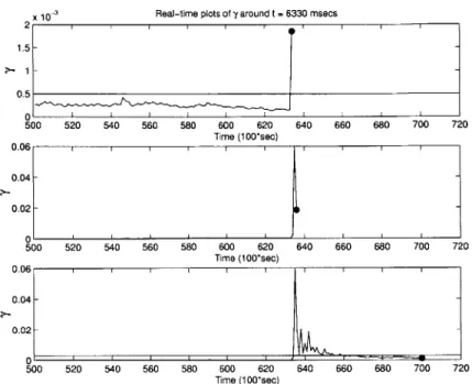
which BEAM detects a system-wide event. Figure 4-3 illustrates the progressive vi-sual output of BEAM when analyzing the A1XOO3 dataset. Note that the middle figure lacks a threshold "bar" since the process is within the buffer. Furthermore, note that the abnormally large "spike" in the third plot of figure 4-3 reflects a re-initialization where the correlation matrix is computed anew. After a system-wide event occurs and BEAM re-initializes it's variables, the first difference matrix is equiv-alent to the first correlation matrix since a previous correlation nmatrix does not exist. Figure 4-4 is the final visual output of 7y.

Comparing the two results: A clear way to compare the two processes' abilities to

track system-wide events is to examine which events are common to both BEAM and PCA and which events are unique to BEAM and PCA. A visual representation, such as the one in figure 4-5, provides an excellent means by which we can compare the outcomes of the two processes. Markers along the 45 degree line denote an event common to both BEAM and PCA. Markers on the x-axis denote events unique to BEAM, and markers on the y-axis denote events unique to PCA. As we can see, events under PCA is a subset of the events under BEAM. The events at 2050 and 38,010 milliseconds were detected by BEAM but not by the PCA method. If we attempt

9

-x 0-3 Real-time plots of y around t = 6330 msecs 2 F 1.5-0.5 0-0.06 0.04 -0.02 -0.06 - 0.04-0.02- _{500 520 540 560 580 600 620 640 660 680 700 720} 500 520 540 560 580 600 620 640 660 680 700 720 Time (100*sec)

Figure 4-3: Real-time plots of -y for the A1X003 dataset

Final plot of y 0.0 0.0 0.0 0.0 0.0 5 - -.-.-- --.- -.-.-4 - - - ---. -. - --.- .. . 3 - - - - - -.-.-. -.- .-- 0 0 500 1000 1500 2000 2500 3000 3500 4000 4500 Time (100*sec)

Figure 4-4: Final plot of -y for the A1XO03 dataset

500 520 540 560 580 600 620 640 660 680 700 720

Time (100*sec)

0

500 520 540 560 580 600 620 640 660 680 700 720

Event comparison plot 5000 - - - --4500 . . ... 4000 3500 - 3000 -2 5 0 0 -- -.-.-..--.-- -.-- -- -- -- --2 0 0 1-5000 - - - -- - - -- - - - --- ..-.. --10 0 0 - --- - -- - - -- - - -- -

-Events under BEAM (100*sec)

Figure 4-5: BEAM vs. PCA in detecting events for the A1X003 dataset

to capture these events under PCA by lowering the thresholds, we begin to detect events that cannot be verified through the test request documentation. For example, if we lower the threshold for the first principal component, the first new event that is captured occurs at 25,440 milliseconds. In addition, if we lower the threshold in the second principal component, the first new event occurs at 43,280 milliseconds. The test request documentation cannot account for either of these events. Therefore, we can state that there is no benefit to using PCA over BEAM in detecting system-wide events that are accountable through the test request documentation. After observing figure 4-5, we can see that the superset of system-wide events occurred at 1250, 2050, 2730, 6330, 34,980, 36,010, 38,010, and 46,010 milliseconds. Section 4.3 will explore the accuracy of these detections when compared with the test request documentation.

4.2.2

Channel Localization and Contribution

Upon detecting a system-wide event, we must localize the sources of these changes. In a 323 channel system, as in the case of the A1XO03 dataset, localizing the possible sources to 10 channels is a fairly efficient reduction in the observable telemetry. The latter equates to a 96.9% reduction in the number of channels one needs to observe

surrounding a specific system-wide event. The following will discuss the methods that were used to localize the sources of events for both PCA and BEAM. Furthermore, in section 4.3, we will compare how effective these localizations were when compared to the information in the test request documentation. But before we proceed, it is important to note that we used the BEAM events as the global list of events for computing channel contribution under both BEAM and PCA. A concern arises when we compute channel contribution around an event unique to BEAM; the calculations under PCA might be unreliable due to the fact that PCA had not signaled an event at that time. We will illustrate this further through an example in section 4.3. Note, however, that the opposite scenario does not exist due to the fact that BEAM events are a superset of PCA events. Unless otherwise noted, we will examine in detail the channel contributions around the system-wide event at 6330 milliseconds for the re-mainder of this section'.

Computing channel contribution under PCA: We developed three methods for

cal-culating channel contribution under PCA. The first method is to simply use the coefficients in the eigenvector of the correlation matrix. For instance, if an event is captured by the nth principal component, then we simply sort the elements of 10,,j

where 0?, is the nth eigenvector. A serious problem arises when we utilize this method.

Since we are often limited to observing the first few significant principal components, we limit our number of possible unique channel contributions. For example, if the first principal component captures three different system-wide events, then all three events will list the same channel contributions because we would use the first eigenvector's

coefficients as the channel contributions for all three events.

The second method, which we will refer to as the 1" order method, simply uses the derivative of the first order principal component. If we let x, be the nth channel, i.e., the n'h column in matrix X of equation 3.1, we can define the difference of xn as

x'n[t] = xn[t + 11 - xn[t]. (4.1)

Then due to linearity, we can compute the difference of the nth principal component via

y'n = On * x'n _(4.2)

where On is the nth eigenvector of the correlation matrix for x. If, for example, the first principal component captured an event at time t, i.e., a sharp impulse above threshold in the derivative of the first principal component, we can calculate how much each channel contributed to that impulse. Let us define c as

C [ X'I[t] * #1[1] x'2[t] * 01[2] X'N[t] * [N] (4.3)

where c[n] is channel n's contribution to the impulse at time t.2 _{In other words,} N

y' [t] E c[n]. (4.4)

n=1

The latter equation simply states that if we sum vector c, we obtain the value of the difference of the first principal component at time t. We can rank the elements of c after taking the sign of the impulse into account. If the impulse is negative, we would place the greatest significance on the most negative element of c.

The third and final method, which we will refer to as the 2nd order window method,

uses windowed principal components to perform the 1s' order method. Given that we have already computed the principal components on the entire dataset, we would use a subset of these principal components to compute a new set of principal components. Let 2A be the length of the window and y, be the nth principal component. In addition, let us say that we want to calculate the channel contribution for an event

2

1n equation 4.3, we need to use the principal component that is responsible for capturing the event. For example, if the event under investigation was captured by the third principal component, we would replace 01[i] with #3[i].

at time t. Then if we define W as

wi[1] W2[11 -.- W N[1

w i[2] W2[2] _{- WN[2}

(4.5)

wl[2A + 1] w2[2.A + 1] ... WN[2A + 1]j

Y1[It -A] Y₂ It - A] Y₃ It - 'A] .. YN[t - A]

Y1

yIt] Y2[It] Y3 It] yNlil

(4.6)

Y1I~t

then we would simply replace x, with we, in equations 4.1 through 4.3 and compute channel contributions as outlined in the 1t order method. There are two opposing factors involved when setting the value of 2A. First, we must maintain a reason-able window size in order to provide enough sample points for computing correlation matrices. Second, we want to avoid or minimize the number of peripheral events occurring within the window so as to maximize the influence of the centered event when computing the 2nd order principal components. For the A1X003 dataset, the

minimum separation between PCA events was 100 samples. However, convention states that we must choose at least 323 samples to compute a correlation matrix for 323 channels. On the other hand, only about 100 channels are active at a given time when we limit our observations to a window of that magnitude. Therefore, we set 2A = 100 samples. Figure 4-6 is the histogram of the ten most significant channels surrounding the event at 6330 milliseconds when using the 2"d order window method.

Computing channel contribution under BEAM: Upon detecting a system-wide event,

BEAM computes in percentage terms how much each channel contributed to that event. Section 3.2.5 outlined in detail the precise method for computing channel con-tribution. Figure 4-7 illustrates the channel contributions around the event at 6330 milliseconds under BEAM.

Histogram of channel contribution at t -6330 msecs under PCA 2.5 I I I I 2-w 1.5- 0.5-0 11 15 138 146 12 16 153 200 70 62 Channel number

Figure 4-6: Channel contributions under PCA

Comparing the two results: In order to compare the channel contribution calculations

from BEAM and PCA, we must look at their relative contributions rather than their absolute contributions. The outputs of BEAM's channel contribution method and PCA's 2nd order method are separated by an order of magnitude, i.e., we cannot

compare the absolute values in figures 4-6 and 4-7. Therefore, we must compare the relative channel contributions. If we are observing the channel contributions around the event at 6330 milliseconds, how do the ten most important channels under the PCA's 2n order method compare to the ten most important channels under BEAM?

Figure 4-8 provides a visual method to compare the relative rankings. The top plot in figure 4-8 is just a normalized superposition of the plots in figures 4-6 and 4-7. In the bottom plot, we are comparing the relative rankings from BEAM and PCA. For in-stance, the channel that contributed the most to the event at 6330 milliseconds under BEAM is the seventh most important contributor under PCA. If all of the rankings from the two processes are identical, all points would lie along the 45 degree line. While the example in figure 4-8 did not produce a perfect match, the importance lies in the fact that the eight most significant channels are common among BEAM and PCA. Further examination will show that all eights channels have identical

charac-Histogram of channel contribution at t -6330 msecs under BEAM I1 I 12- 10-8 6-4 2-0 153 200 12 16 138 146 11 15 258 283 Channel number

Figure 4-7: Channel contributions under BEAM

teristics around the event at 6330 milliseconds. Figure 4-9 contains the plots of three of the eight channels involved. We can clearly see that all three channels behave identically at 6330 milliseconds. Therefore, while an identical match along the 45 de-gree line would be ideal, a closer examination of the actual channel data reveals that localizing our attention to a small group of channels will suffice. We only care that both BEAM and PCA were able localize our attention to the same eight channels. An exhaustive search among the remaining 315 channels revealed that other channels were barely, if at all, involved in this event. We obtained similar results when we calculated, ranked, and compared channel contributions around the remaining seven events [see Appendix A].

4.3

Test Request Benchmark

Let us now turn to the test request documentation to verify the results from analyses performed on the A1XO03 dataset. We pointed out earlier that system-wide events under BEAM were a superset of events under PCA. Therefore, we can come to one of three possible conclusions. First, both BEAM and PCA lacked the sensitivity to

Channel contributions to event at t = 6330 msecs 6 6 A A A BEAM 0 PCA o o -- -- - - -- - -- - - A - A - -- -- - - - -e - - - A 1 2 3 4 5 6 Significant channels 0 1 2 3 4 5 6

Ranking from BEAM

7 8 9 10

7 8 9 10

Figure 4-8: Comparison of the 10 most significant channels under BEAM and PCA.

Channel 11 4 2-0- --2 Channel 153 0 0.5 --1 - 0--0.5 - -1-600 610 620 630 Time (100*secs)

I

Figure 4-9: Plots of three channels surrounding the event at 6330 msecs.

C I 0.5 -3 -1 --1.5 -10 a 0 E 6 4 2-. . . . .. .. . .-- --- - - 0- -- --- - -- - --- - --- -- --- - - 0 --- - --- --- --- --- --- -- - - 0 - - - - - -o

--/