HAL Id: hal-00395876
https://hal.archives-ouvertes.fr/hal-00395876
Submitted on 18 Oct 2012
HAL is a multi-disciplinary open access
archive for the deposit and dissemination of sci-entific research documents, whether they are pub-lished or not. The documents may come from teaching and research institutions in France or abroad, or from public or private research centers.
L’archive ouverte pluridisciplinaire HAL, est destinée au dépôt et à la diffusion de documents scientifiques de niveau recherche, publiés ou non, émanant des établissements d’enseignement et de recherche français ou étrangers, des laboratoires publics ou privés.
Probability weighting and the ’level’ and ’spacing’ of
outcomes: An experimental study over losses
Nathalie Etchart-Vincent
To cite this version:
Nathalie Etchart-Vincent. Probability weighting and the ’level’ and ’spacing’ of outcomes: An exper-imental study over losses. Journal of Risk and Uncertainty, Springer Verlag, 2009, 39 (1), pp.45-63. �10.1007/s11166-009-9066-0�. �hal-00395876�
Probability weighting and the ‘level’ and ‘spacing’ of outcomes:
An experimental study over losses
Nathalie Etchart-Vincent
Centre National de la Recherche Scientifique (CNRS),
Centre International de Recherche sur l’Environnement et le Développement (CIRED),
Campus du Jardin Tropical,
45 bis, Avenue de la Belle Gabrielle,
94736 Nogent sur Marne Cedex, France
Abstract: The main goal of the experimental study described in this paper is to investigate the
sensitivity of probability weighting to the payoff structure of the gambling situation – namely the
level of consequences at stake and the spacing between them – in the loss domain. For that
purpose, three kinds of gambles are introduced: two kinds of homogeneous gambles (involving
either small or large losses), and heterogeneous gambles involving both large and small losses.
The findings suggest that at least for moderate/high probability of loss do both ‘level’ and ‘spacing’ effects reach significance, with the impact of ‘spacing’ being both opposite to and
stronger than the impact of ‘level’. As compared to small-loss gambles, large-loss gambles
appear to enhance probabilistic optimism, while heterogeneous gambles tend to increase
pessimism.
Keywords: Individual decision making under risk, Prospect theory, Losses, Probability weighting
A huge body of experimental as well as field evidence has demonstrated the descriptive
weaknesses of the expected utility (EU) model. Among the most promising challengers to EU,
the rank-dependent family includes rank-dependent utility – denoted RDU (Quiggin, 1982) – and
(Cumulative) Prospect Theory – simply denoted PT (Tversky and Kahneman, 1992). The
satisfactory descriptive power and growing popularity of these models are closely linked with
their typical ‘dual’ structure, which is intended to mimic the intuitively ‘dual’ structure of risk
attitude, decomposing in attitude towards probability and in attitude towards consequences
(Wakker, 1994). Like EU, RDU and PT capture sensitivity towards outcomes through a utility
function1. But unlike EU, they also model subjectivity toward probability (which can be called
probabilistic risk attitude) through a probability weighting function2. Probability weighting has
received many interpretations. It can be seen as either irrational (McFadden, 1999) or
self-regulatory and adaptative (Higgins, 1997, 1998, 2000; Kluger et al., 2004). It may also capture
the psychophysics of chance (Kahneman and Tversky, 1984; Gonzalez and Wu, 1999) as well as
some strategic attitude towards probabilistic risk (Wakker, 2004).
The probability weighting function has been extensively investigated, both theoretically
(e.g. Diecidue, Schmidt and Zank, 2007; Prelec, 1998) and empirically. Whatever the domain
(either gains or losses) under investigation, the most typical and widely replicated result is the
inverse-S shape of the probability weighting function at the aggregate level (Abdellaoui, 2000;
Lattimore, Baker and Witte, 1992; Tversky and Kahneman, 1992). However, note that some
1 The utility function in the PT model actually exhibits some peculiar features, and it has been given a different
name (the value function). Since these features do not matter here, the usual 'utility' name will still be used throughout the paper (see Fennema and Van Assen, 1999).
2 In both RDU and PT, the weighting function is used to build the decision weight associated to each consequence
using a rank-dependent combination rule, from which the rank-dependent designation (for some details on this point, see Gonzalez and Wu, 1999, p. 135-136 and Diecidue and Wakker, 2001; for a general discussion about probability weighting, see Neilson, 2003).
recent studies found S-shaped median functions (e.g. Alarié and Dionne, 2001; Humphrey and
Verschoor, 2004; Harbaugh, Krause and Vesterlund, 2002) and, above all, that huge
heterogeneity prevails at the individual level. For instance, probability weighting has been shown
to depend on the respondents’ socio-demographic characteristics (such as gender, e.g.
Fehr-Duda, de Gennaro and Schubert, 2006; or age, e.g. Harbaugh, Krause and Vesterlund, 2002) as
well as on their emotional state and mood (e.g. Fehr et al., 2007). It has also been shown to be
affected by some features of the gambling situation, such as the emotional content of the payoffs
(e.g. Rottenstreich and Hsee, 2001) or their gain/loss nature (e.g. Abdellaoui, 2000).
Besides, there is also some suggestive evidence that, within a given payoff domain, the
probability weighting function be sensitive to the payoff structure of the gambling situation. This
result cannot be reconciled with either RDU or CPT3. As Tversky and Kahneman (1992)
suggest, "despite its greater generality, the cumulative functional is unlikely to be accurate in
detail. We suspect that decision weights may be sensitive to the formulation of the prospects, as well as to the number, the spacing and the level of outcomes. In particular, there is some evidence to suggest that the curvature of the weighting function is more pronounced when the outcomes are widely spaced" (p. 317, underlined by the author). The sensitivity of probability
weighting to the payoff structure of the gambling situation has actually been indirectly shown in
some laboratory studies (Allais, 1988, p. 243; Camerer, 1992, p. 237; Harless and Camerer,
1994, p. 1282; Sonsino, 2008, p. 379) and it has been documented outside the laboratory as well.
For instance, probabilities seem to be all the more optimistically [resp. pessimistically]
overweighted since they are associated with especially desirable consequences (Irwin, 1953;
3 Note that some generic rank-dependent models allow probability weighting to be affected by the payoffs (Green
and Jullien, 1988; Quiggin, 1989; Segal, 1989, 1993; see also Quiggin, 1993). Besides, Viscusi’s prospective reference theory (Viscusi, 1989) allows probabilities to depend on the number of the payoffs, but not on the ‘level’ and ‘spacing’ of these payoffs.
Rosett, 1971; Slovic, 1966) [resp. negative consequences; Viscusi, 1995]. But I am aware of only
one specifically dedicated experimental study (Etchart-Vincent, 2004, in this journal), that was
designed to investigate the impact of the magnitude (i.e. the ‘level’) of the payoffs on probability
weighting in the loss domain. Etchart-Vincent (2004)’s findings suggest that people tend to be
more pessimistic when facing large losses rather than small ones. However, Tversky and Kahneman (1992)’s above-quoted passage suggests that the payoff structure of a risky gamble
should not be reduced to the ‘level’ of the outcomes. Their ‘spacing’ is also likely to affect
probability weighting. And my expectation is that it might result in stronger probabilistic
pessimism (as well as, consequently, in more risk aversion4).
An example derived from the insurance field may help grasp the importance of the ‘spacing’ hypothesis. Indeed, taking out an insurance does not only considerably reduce the
magnitude of the potential loss, it also – and perhaps above all – reduces the gap between the
most and the least serious consequences in the corresponding lottery (with probabilities being
held constant). Instead of losing, say, either US$ 10 000 (in case damage occurs, with a
probability of 0.01 for instance) or 0 (with a probability of 0.99), the insured individual will now
lose, say, either US$ 750 if damage occurs (corresponding to the payment of an insurance
premium and a deductible) or US$ 200 (corresponding to premium only) if not. Insurance
purchase thus roughly induces the replacement of highly heterogeneous Lottery A = (–US$ 10
000, 0.01; 0) with rather homogeneous Lottery B = (–US$ 750, 0.01; –US$ 200). My expectation
is that this significant reduction in loss heterogeneity might result in lower probability
overweighting (or, if we retain the most usual interpretation of probability weighting in the PT
4 Note that the opposite idea of ‘probability neglect’ (Sunstein, 2003) also predicts that individuals will be more risk
averse when facing the possibility of an extremely low probability-extremely large loss event (e.g. a terrorist attack). In that case indeed, people will focus on the badness of the outcome rather than on the (low) probability with which the outcome is supposed to occur. Therefore, this event will have much stronger negative impact than would have been expected given the objective value of the risk.
framework, in weaker probabilistic pessimism). This may in turn induce a lower degree of risk
aversion, or even some proneness to risk seeking, and finally explain why some people tend to
take more risks when being insured (Cummins and Tennyson, 1996). Interestingly, the ‘spacing and level’ hypothesis allows us to regard the risk taking behaviour of insured people as cognitive
and possibly unintentional, instead of deliberate and opportunistic – as usually done in the ‘moral hazard’ literature.
The present experimental study primarily aims at investigating whether and how
probability weighting is to be affected by the payoff structure of the gamble, and at disentangling
the respective effects of ‘level’ and ‘spacing’5. The experimental framework we have chosen to
develop for that purpose is thus similar to, but more integrating than, the one that was used in
Etchart-Vincent (2004).
To be specific, the study is based on a two-stage semi-parametric choice-based procedure.
In the first stage, each subject’s utility function is elicited on a wide interval of losses I, using the
non-parametric trade-off method (Wakker and Deneffe, 1996). In the second stage, three
different loss situations are considered. The first two situations, called the ‘small loss’ and ‘large loss’ situations respectively, involve lotteries made up of either small losses (at the upper part of
I) or large losses (at the lower part of I). The third situation involves heterogeneous gambles, i.e.
gambles that offer both a small loss (at the upper bound of I) and a large one (at the lower bound
of I). A simple certainty-equivalent method is then used to elicit, within the PT framework, the subject’s probability weighting function in each of the three loss situations.
5 As a worthwhile by-product, the experimental design also allows us to investigate the subjects’ risk attitude
depending on the payoff structure of the gambling situation, as well as the subjects’ utility function on a wide interval of losses. For the sake of clarity, only the results concerning probability weighting will be reported here.
The main results are as follows. At least for moderate and high probability of loss, the
weighting function appears to be affected by the payoff structure of the prospects. Besides, ‘level’ and ‘spacing’ appear to have rather opposite effects: as compared to small loss prospects,
large loss gambles tend to induce less probability overweighting (i.e. either less pessimism or
more optimism), while heterogeneous prospects tend to increase probability overweighting (i.e.
to generate either more pessimism or less optimism).
The remainder of the paper is organized as follows. Section 1 is devoted to the set out of
the two-stage method used to successively elicit the utility and weighting functions. The
experimental design is described in Section 2. Section 3 reports the results, which are further
discussed in Section 4. Section 5 concludes.
1. Method
First, just recall that the PT model introduces two different weighting functions depending
on the domain of consequences. They are denoted w+ and w- for the gain and loss domains
respectively. In the simplified framework of a two-outcome non-zero lottery P = (x2, p; x1)with
x2 < x1 < 0, the PT valuation of P is given by VPT(P) = w-(p)U(x2) + (1– w-(p))U(x1), where U is
the utility function. Besides, the PT valuation of a mixed lottery P = (x2, p; x1, 1– p) with x2 > 0
> x1 is given by VPT(P) = w+(p)U(x2) + w-(1– p)U(x1).
Now, let us present the basic principles of the two-stage semi-parametric procedure that
was used to elicit the probability weighting functions at the individual level. It is basically the
same as in Etchart-Vincent (2004). First, the utility function was elicited for each subject, using
the now well-established non-parametric trade-off method (introduced by Wakker and Deneffe,
1996 and applied to losses by Abdellaoui, 2000; Etchart-Vincent, 2004; Fennema and Van
well as large losses (until around 15 000 €). But in the 2004 study, only two distinct local parts
of the utility function were obtained. Here, utility was elicited on a unique and wide interval I,
enabling us to work with heterogeneous lotteries within this interval. In the second stage of the
procedure, a certainty-equivalent method was introduced, using some points of the previously
elicited utility function as well as its parametric fitting, to build the weighting function in each of
three loss situations, called the ‘small loss situation’ (S), ‘large loss situation’ (L) and
‘small-large loss situation’ (S/L) respectively.
Let us briefly recall the main features of the trade-off (TO) method. This method consists
in eliciting a sequence of outcomes that are equally spaced in terms of utility. Using its more
reliable ‘outward’ version (see Fennema and van Assen, 1999), the general principle of the
method is the following. Given fixed outcomes x0, r and R such that x0 < 0 < r < R, the subject is
asked to make successive choices allowing (through a l-iterations bisection process) to determine
the outcome x1 < x0 that makes her indifferent between the (mixed) lotteries (x0, p; r, 1– p) and
(x1, p; R, 1–p). Then, x1 is used as an input, and a similar choice-based bisection process allows
to determine the outcome x2 < x1 that makes the subject indifferent between (x1, p; r, 1–p) and
(x2, p; R, 1–p). The procedure is implemented n times in order to obtain a sequence xn, …, xi, …,
x0. Under PT, indifference between (xi, p; r, 1–p) and (xi+1, p; R, 1–p) implies that, for 0 ≤ i ≤
n-1, w-(p)U(xi) + w+(1–p)U(r) = w-(p)U(xi+1) + w+(1–p)U(R). In other words:
U(xi) – U(xi+1) = (w+(1–p)/ w-(p))[U(R) – U(r)] for all 0 ≤ i ≤ n-1 Eq. (1)
, from which the following equality: +
U(x0) – U(x1) = U(x1) – U(x2) = … = U(xi) – U(xi+1) = … = U(xn-1) – U(xn) Eq. (2).
Eq. (2) implies that, for the subject under consideration, the x-is are equally spaced in terms
of utility. Using the conventional normalization U(x0) = 0 and U(xn) = –1, one gets U(xi) = – i/n,
elicitation process. It thus avoids those biases that are due to probability weighting and are
known to distort traditional assessment methods (see Wakker and Deneffe, 1996 for a critical
review of these methods)6.
Now, let us present the general principle of the certainty-equivalent method that was used
in the second stage of the procedure to build the weighting function under a given payoff
condition: the decision maker is asked to make successive choices allowing – at the end of a
m-iterations bisection process – to determine the value CEj that makes her indifferent between
two-outcome Lottery A = (xk, pj; xi, 1–pj), with xk and xi two elements of the former standard
sequence and xk < xi < 0, and degenerate Lottery B = (CEj, 1). In generic Lottery A = (xk, pj; xi,
1–pj), k and i can be chosen so as to make xk and xi eligible as bounds of the payoff condition
under consideration. By construction, xk < CEj < xi.
Under PT, and with xk < xi < 0, the indifference between (xk, pj; xi, 1–pj) and CEj entails
that w-(pj)U(xk) + (1–w-(pj))U(xi) = U(CEj). By construction of the TO method, U(xi) = –i/n and
U(xk) = –k/n. So: k i i ) nU(CE ) (p w j j Eq. (3)
The procedure thus makes it possible to determine algebraically the ‘subjective weight’ w
-(pj) for any probability pj. By applying it for different values of pj, the whole weighting function
can be obtained under the payoff condition given by [xk; xi].
6 Note that the TO method may suffer from two drawbacks (see Wakker and Deneffe, 1996). First, it induces a bias
toward linearity. Therefore, it should not be used to elicit the utility function over a small interval of consequences. In this study, the elicitation process involves a wide interval of losses, which prevents this problem. Second, the TO method is chained. So any early error in the elicitation process will propagate and distort subsequently elicited utility values. However, several studies have investigated this point and shown that the impact of error propagation can be considered as negligible (Abdellaoui, Vossman and Weber, 2005; Bleichrodt and Pinto, 2000).
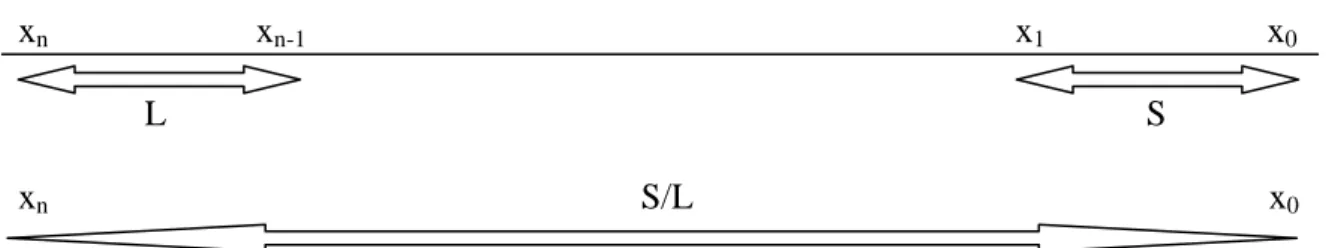
In the present study, the weighting function had to be built under each of the S, L and S/L
payoff conditions. In each case, the points (of the previously elicited standard sequence) xk and
xi had to be properly chosen so as to be eligible as the bounds of the payoff condition under
consideration. So, S was defined by k=1 and i=0, L by k=n and i=n–1, and S/L by k=n and i=0
(see Figure 1). Note that, even though k and i were the same for all the subjects, the values xk and
xi were specific to each subject (since they were elements of her endogenously elicited utility
function).
[INSERT FIGURE 1 ABOUT HERE]
The interest of the above-described procedure is that it makes it possible to roughly disentangle the ‘level’ effect from the ‘spacing’ effect7
. Indeed:
- w
-Land w-S/Lwere both obtained using the last point of the standard sequence xn. But in the L
situation, the alternative consequence was xn-1, instead of x0 in the S/L situation. The
comparison between w-L and w-S/L thus makes it possible to investigate how probability
weighting is to be affected by the ’spacing’ of consequences.
- w
-L and w-S were both constructed using homogeneous lotteries. Indeed, the distance (in
terms of utility) between xn and xn–1 is (by construction) subjectively equivalent to the
distance between x1 and x0. By neutralizing the ‘spacing’ effect, the comparison between the
functions w-Land w-Sthus makes it possible to investigate the sole impact of the absolute
level of consequences.
At this stage, an important point to make is that certainty equivalents CEjs are unlikely to
be elements of the previously elicited standard sequence. So the U(CEj)s and w-(pj)s could not be
7 Roughly, since it is actually impossible to completely control the way subjects perceive a loss situation that is
obtained without fitting U parametrically, from which the name of ‘semi-parametric’ procedure8.
Moreover, U needed be especially well fitted to allow reliable calculations using Eq. (3). This is
why each individual utility function was fitted using 3 different specifications, and for each
subject the best fitting specification was retained. The first two – standard – specifications are
the one-parameter POWer function, with UPOW(x) = –(–x)and >0 (Tversky and Kahneman,
1992) and the two-parameter EXpo-POWer function, with UEXPOW(x) = [1–exp(–(–x))]/(exp(– )–1), >0 and >0 (Abdellaoui, Barrios and Wakker, 2007; Saha, 1993)9.
The third specification is more unusual. Denoted GE (with reference to Goldstein and
Einhorn, who introduced it in their 1987 paper), it is given by UGE(x) = γ γ γ x) (1 x) δ( x) δ( , with
>0 and >0. Because it allows inverse-S shape, this specification has been extensively used in the literature to fit probability weighting functions. Since 25% of our individual utility functions
exhibited an inverse-S shape10, the GE specification was used for the pragmatic purpose of best
fitting.
2. Experimental design
30 subjects participated in the final experiment. All of them were undergraduate
wage-earning students at the Department of Economics and Management at ENS de Cachan (France).
They all had some background in probabilities, but none of them had followed any specific
8
Linear interpolation could not be used here, neither for replacing estimation as in Abdellaoui, Attema and Bleichrodt (2008), nor for checking estimation reliability as in Bleichrodt and Pinto (2000). Indeed, the rather big distance between two successive points of the standard sequence made it impossible to assume linearity between them (see Wakker and Deneffe, 1996).
9 Note that EXPOW reduces to POW when tends to 0.
course on decision theory. They were paid for participation (they received a flat-rate of 15 €,
around US$ 20) but no performance-based payment was used. The reason for this is twofold.
First, subjecting volunteers to the possibility of losing ‘for real’ is both ethically questionable
and practically impossible (Mason et al., 2005, p. 189 note 4), a fortiori when losses at stake are
large. Second, the most widely used alternative option, namely the ‘initial endowment’
strategy11, may give rise to several detrimental biases, among which the famous ‘house money effect’ (Boylan and Sprinkle, 2001; Keasy and Moon, 1996; Thaler and Johnson, 1990; Weber
and Zuchel, 2005). Fortunately, there is some suggestive evidence that the use of real monetary
incentives does not significantly affect the findings when the subject’s task consists in choosing
between simple lotteries (Beattie and Loomes, 1997; Bonner et al., 2000; Bonner and Sprinkle,
2002; Camerer and Hogarth, 1999; Etchart-Vincent and L’Haridon, 2008; Hertwig and Ortmann,
2001).
Now, the experiment consisted in two successive computerized sessions. Each subject
was individually interviewed in the presence of the experimenter. The utility (resp. probability
weighting) function was elicited in the first (resp. second) session. A break separated the
sessions. Each interview lasted between 45 and 75 minutes. All along the experiment, the subject
was only asked to make choices between lotteries, displayed as pie charts on a computer screen
(both consequences and probabilities were stated explicitly; see Etchart-Vincent, 2004,
Appendix A for a typical computer screen12). Indeed, choice-based procedures have proven to be
easier for the subjects and to produce more reliable data than direct matching (Bostic, Herrnstein
and Luce; 1990; Tversky, Sattah and Slovic, 1988). A 6-iterations bisection process was used to
obtain all the indifference points.
11 This strategy consists in providing the subjects with an initial endowment from which they can lose some money
during the experiment. The idea is to make them suffer real losses, but not from their own pockets.
In the first stage of the procedure, p = 0.33 was chosen to elicit the utility function at the
individual level, in accordance with Wakker and Deneffe (1996, p. 1144)’s suggestion. In former
studies, p was given either the value 0.5 (Bleichrodt and Pinto, 2000), 0.33 (Fennema and Van
Assen, 1999) or 0.67 (Abdellaoui, 2000). The pilot experiment was used to calibrate the starting
point of the standard sequence x0, the reference outcomes r and R (with x0, r and R being fixed
and common to all subjects), and the number of points n, so as to get for x1 (resp.xn) a mean
value around a month earnings (resp. around the price of a medium-sized car). n = 6 was finally
chosen, as well as x0 = –150 € (–US$ 200), r = 300 €(US$ 400) and R = 1500 € (US$ 2 000).
Finally, the calibration process was rather successful, since the mean values obtained for x1 and
x6 on our 30-subject sample were –1265 € (–US$ 1 750) and –12 850 € (–US$ 17 700)
respectively. Of course, huge heterogeneity prevailed at the individual level, resulting in lower
median values: median x1 was around – 800 € (–US$ 1 100, while median x6 was around –7 600
€ (–US$ 10 500).
In the second stage of the experiment, the three payoff conditions S, L and S/L were
defined by the intervals [x1; x0], [x6; x4]13 and [x6; x0] respectively (see Section 1 and Figure 1
supra)14. In each payoff condition, the same 6 probabilities pj = 0.01, 0.1, 0.25, 0.5, 0.75, and 0.9
were chosen for the probability weighting elicitation work. The order in which the S, L and S/L
loss situations were shown to the subjects, as well as the order in which probabilities were
displayed within each situation, were randomized to prevent any order effects. As usual, a
practice session was introduced prior to the experiment, as well as consistency checks after it.
Since loss situations have proven to be psychologically and cognitively hard to deal with, the
13 The pilot experiment showed that the theoretically appropriate interval [x
6; x5] was actually too small to allow the
subjects to reliably determine several certainty equivalents within its bounds.
14 Remember that the three values x
1, x4 and x6 were endogenously determined using the TO method, thus specific to
practice session and the break during the experiment also aimed to make the task more
comfortable for the subjects.
Now, as regards the subjects’ internal consistency, it was checked through the systematic
repetition of the ith (out of 6) iteration in each choice situation, with i = 4 for the elicitation of
both the utility function and the probability weighting function in the S and L situations, and i =
5 for the elicitation of the probability weighting function in the S/L situation (because of the
greater width of the interval of consequences in this case). The 6 points of the standard sequence
thus provided 6 individual internal consistency checks for utility. Similarly, the 6 certainty
equivalents obtained in S (resp. L, S/L) provided 6 individual consistency checks for probability
weighting in S (resp. L, S/L). The percentage of consistent choices among our subjects was then
computed to obtain four average consistency rates – 80% for S, 71% for S/L, 72% for both utility
and L – which appear to be in line with those obtained in similar previous studies (see for
instance Abdellaoui, 2000; Abdellaoui, Bleichrodt and L’Haridon, 2008; Camerer, 1992).
3. Results
3.1. Non-parametric and parametric tools
Probability weighting functions can be first investigated in terms of
underweighting/overweighting. Following the usual interpretation of probability weighting in
terms of optimism/pessimism, a decision maker is said to be optimistic (resp. pessimistic) if her
weighting function over losses exhibits under (resp. over)-weighting, i.e. if w-(p) < p (resp. w-(p)
> p) for all p (e.g. Cohen, 1994).
Weighting functions can also be described through their main two physical features,
probability weighting (Gonzalez and Wu, 1999; Starmer, 2000; Tversky and Kahneman, 1992;
Tversky and Wakker, 1995). On the one hand, elevation captures the ‘attractiveness’ of the
gamble for the subject under consideration: her weighting function w- will be all the higher (resp.
lower) since she considers the gamble as more repulsive (resp. attractive). Note that the concepts
of attractiveness/repulsiveness are close to those of optimism /pessimism.
On the other hand, curvature reflects ‘discriminability’ (between probabilities). The most
usual interpretation of discriminability is a cognitive one. It is meant to capture the decision
maker’s limited ability to discriminate between probabilities: the higher this ability, the more
linear the weighting function. Ability to discriminate is closely related to the ‘diminishing
sensitivity’ principle; it is all the lower since probability is remote from the natural bounds 0 and
1 (Tversky and Kahneman, 1992). It is also connected with the decision maker’s familiarity with
the risky situation under consideration. High familiarity/competence may counterbalance or even
prevent diminishing sensitivity. However, discriminability may also be viewed as strategic. In
this approach, the decision maker will deliberately give the same weight to different
probabilities, because she needs not differentiate between them in order to take a satisfactory
decision. The strategic approach thus assumes that the subject adapts her cognitive effort to her
needs at the end of a kind of implicit cost-benefit analysis. The comments made by our subjects
during the experiment suggest that the cognitive and strategic interpretations should be viewed as
complementary rather than exclusive. Still, in order to avoid ambiguity, only the descriptive term ‘discriminability’ will be retained here when reporting the results.
Some two-parameter specifications allow to capture both curvature and elevation, each
parameter governing (as independently as possible) one feature. The most popular specification,
denoted GE and such that wGE(p) = γ γ γ p) (1 δp δp
, was first suggested by Goldstein and Einhorn
(1987) and then used by Lattimore, Bakker and Witte (1992), Tversky and Fox (1995) and
the specification denoted PREL and such that wPREL(p) = exp(–(–log(p)), where parameters get
the same interpretation as in GE. In both GE and PREL, governs elevation. Under PT over losses, < 1 (resp. > 1) implies absolute attractiveness (resp. repulsiveness). governs curvature and gives some information about discriminability: the nearer to 1 is, the flatter the curve and the higher discriminability. Besides, < 1 generates the usual inverse-S shape. The comparison between two weighting functions w-1 and w-2 is thus reducible to the comparison
between parameters 1 and 2 on the one hand, and between 1 and 2 on the other hand.
Note that some single-parameter specifications have also been used in the literature. Tversky and Kahneman (1992)’s specification, denoted TK and such that wTK(p) =
1/
p [(p (1 p)]
, is the most popular one. However, unless discriminability and attractiveness covary so that they can be encapsulated in a single parameter – which unfortunately is unlikely
to happen (Gonzalez and Wu, 1999) – the descriptive power of such specifications appears to be
questionable, especially on individual data. In the following, parametric fitting of the median
probability weighting functions using TK will nevertheless be reported, for the purpose of
comparison with previous studies.
3.2. The ‘level’ and ‘spacing’ effects
Both two-tailed paired t29-tests and Wilcoxon tests were run to analyse the data. Since they
always give similar results, only the former will be presented here.
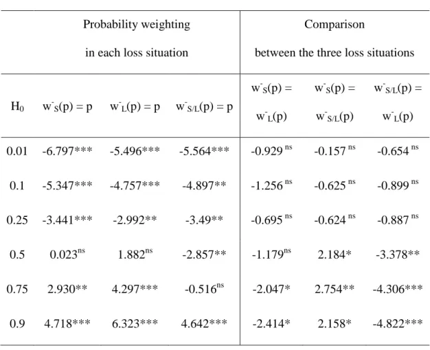
The left part of Table 1 reports the results of two-tailed paired t29-tests as regards basic
probability weighting (H0: w-(p) = p). Unsurprisingly, the usual inverse-S shape is replicated.
probability overweighting than in S and L: in S/L, the only underweighted probability is 0.9 and ‘low’ probabilities until 0.5 are significantly overweighted.
[INSERT TABLE 1 ABOUT HERE]
Now, as regards the comparison between w-S, w-L and w-S/L, only for high probabilities
does the difference between w-S and w-L reach significance, with large losses inducing more
underweighting than small ones (right part of Table 1). This suggests that, when the ‘spacing’
effect is controlled, only near certainty does the absolute level of consequences markedly affect
probability weighting.
The ‘spacing’ effect appears to be both stronger than and opposite to the ‘level’ one. First,
only for low probability of loss (p 0.25) does the distance (‘spacing’) between consequences seem not to affect probability weighting. Second, as probability grows, the fact that a large loss
be associated with a small one (S/L) rather than with another large one (L) leads to significant
probability overweighting, instead of significant underweighting.
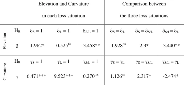
Now, what about parametric estimates? Two-tailed paired t29-tests suggest that the
elevation parameter is not significantly different from 1 in both S and L situations, while S/L
appears to be significantly superior to 1, confirming the repulsive status of heterogeneous
gambles (Table 2, left part).
[INSERT TABLE 2 ABOUT HERE]
As regards curvature, is dramatically inferior to 1 in both S and L, indicating very low discriminability between probabilities when only homogeneous losses are involved. By contrast,
S/L-type heterogeneous prospects appear to increase discriminability, with S/L being only
slightly inferior to 1. This finding is confirmed through direct comparison between the three loss
situations (Table 2, right part). First, neither curvature nor elevation appears to significantly depend on the ‘level’ of consequences. Second, the data suggest that a genuine ‘spacing’ effect is
at play: both elevation and curvature are significantly higher when the prospects are
heterogeneous rather than homogeneous.
Median results may help summarize those obtained at the individual level. The median
values of individual subjective weights, obtained for each probability and loss situation, were
used to build the three median weighting functions w-S, w-L and w-S/L. These three functions
appear to exhibit the expected shape, with significant overweighting of low probabilities and
underweighting of high probabilities (see Figure 2). Moreover, w-S/L (resp. w-L) globally appears
to exhibit the highest (resp. lowest) curve. But only for intermediate and high probabilities does
the difference between the curves look significant.
[INSERT FIGURE 2 ABOUT HERE]
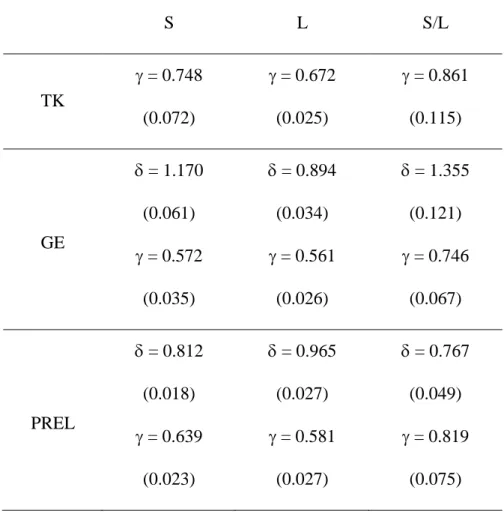
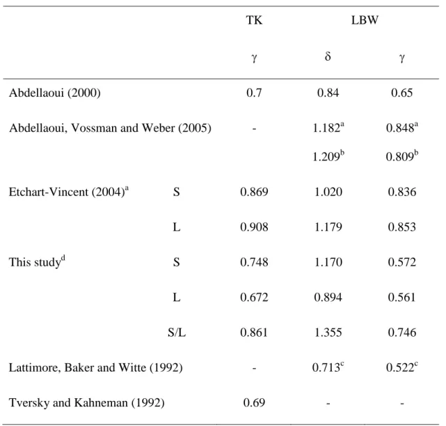
Parametric fitting of the three median weighting functions was achieved using TK, GE and
PREL specifications (see Table 3). For the sake of comparison with previous studies, Table 4
presents both the estimates obtained on our median weighting functions using the one-parameter
TK and two-parameter GE specifications and those obtained with the same specifications by
Abdellaoui (2000), Abdellaoui, Vossman and Weber (2005), Etchart-Vincent (2004) and
Lattimore, Baker and Witte (1992).
[INSERT TABLE 3 ABOUT HERE]
[INSERT TABLE 4 ABOUT HERE]
It is interesting to note that our TK estimates are very similar to Tversky and Kahneman
(1992)’s and Abdellaoui (2000)’s, except for S/L. This finding suggests that something specific
happens when the prospects are heterogeneous. It is also worth noticing that, as compared to
those obtained in Etchart-Vincent (2004), the present fitting results for w-S and w-L look more
standard. It retrospectively appears that the S and L payoff conditions introduced in our 2004
contradiction between both series of results, as well as the remarkable similarity between
previous fitting results for w-L and present fitting results for w-S/L.
Now, what about GE estimates? First, as regards elevation, S and S/L (resp. L) appear to
be considered by the median subject as absolutely repulsive (resp. attractive), and S/L as the
most repulsive situation (S/L > S > 1 > L). Besides, the degree of elevation is significantly
higher than in Abdellaoui (2000) and Lattimore, Bakker and Witte (1992), but it is rather similar
to that found by Abdellaoui, Vossman and Weber (2005) and Etchart-Vincent (2004).
Now, as regards discriminability, < 1 in all cases, which confirms the inverse-S shape of the three curves. Moreover, L < S << S/L < 1, which suggests that discriminability is much
higher in risky situations with widely spaced consequences (S/L) than in situations with
homogeneous consequences, especially when those are large (L). Still, the fact that parameter remains quite low in the three situations indicates that discriminability in the loss domain is
rather poor. Though lower than those found by Etchart-Vincent (2004), the values taken by
parameter in this study are rather close to Abdellaoui (2000)’s and Lattimore, Baker and Witte (1992)’s.
4. Discussion
4.1. Discussion of the method
The method used in this paper may suffer from two main drawbacks. The first potential
difficulty concerns the utility elicitation process. Indeed, the TO method requires that probability
weighting be constant all along the elicitation process, so that (1–w+(p))/w-(p) be constant.
Otherwise, it is no longer possible to get Eq. (2) from Eq. (1) and to use Eq. (2) to build the
outcomes r and R remain the same all along the process while the xis are getting more and more
negative implies that the distance between the consequences at stake increases during the
elicitation process. So, if probability weighting appears to be affected by a ‘spacing’ effect, then
the standard sequence obtained using Eq. (2) is likely to be biased.
To control this problem, a multifaceted strategy was adopted. A first precautionary
measure was to choose a relatively neutral probability for utility elicitation. 0.33 is usually
considered as such: on aggregate data at least, w(0.33) has empirically been shown to be very
close to 0.33 (see Prelec, 1998 for instance), and there is also some evidence that w-(0.33) is not
affected by the payoff structure of the prospects (Etchart-Vincent, 2004). Second, the pilot
experiment gave us some insight into the way the subjects were making their decisions during
the utility elicitation process: it seems that, since the probability p was held constant throughout
the process, the subjects integrated it at first and did not reconsider it later. Such an attitude is
consistent with the intuition that the trade-off method focuses attention on utility and makes
probability a rather secondary choice dimension (see Wakker and Deneffe, 1996, p. 1148).
Thirdly, some subjects took part in both this study and the 2004 one. The remarkable similarity
between the utility functions they produced on these occasions15 suggests that the present
procedure did not suffer from substantial biases16.
The second potential drawback of the method originates from the fact that each w-(pj)
was calculated from a unique certainty equivalent CEj – and more precisely from its utility
U(CEj). Thus, any error in the evaluation of U(CEj), be it due to the poor parametric fitting of the
utility function U or to some bias in the determination of CEj, would directly result in a biased w
15 Note that two years elapsed between the first and the second studies, so that no memory effect can be suspected to
have affected the second set of data.
16 The procedure used in the 2004 study was not concerned with the problem under discussion here. This is why it
(pj). I was highly aware of this potential difficulty and took special care to collect high-quality
data and make good parametric fitting (see Section 1, supra).
4.2. Discussion of the results
The findings suggest that, at least for moderate/high probability of loss, the ‘level’ and ‘spacing’ effects do reach significance, with the impact of ‘spacing’ being both opposite to and
stronger than the impact of ‘level’. In Etchart-Vincent (2004), large-loss gambles appeared to
increase pessimism as compared to small-loss ones, suggesting a pessimistically-oriented ‘level’
effect. So the ‘level’ effect found in the present study appears to be somewhat contradictory to
that obtained in our previous study. This may be due to the fact that, even though
Etchart-Vincent (2004) intended to investigate the sole impact of ‘level’, the gambles involved in that
study were probably not homogeneous enough to prevent any ‘spacing’ effect. So the observed ‘level’ effect was actually a mix of genuine ‘level’ and ‘spacing’ effects, which the present study
precisely shows to be both conflicting and of unequal intensity17.
Another noticeable result of the paper is the quite low degree of curvature
(discriminability) exhibited by individual weighting functions. It may be due to the fact that both
cognitive ability and strategic effort to discriminate be lower in the loss domain than in the gain
domain. First, the subjects are likely to be less familiar with losses than with gains, which may
lessen their ability to discriminate. In this respect, if we admit that probability processing is
facilitated when the gamble situation itself is cognitively easier to deal with (which is the case
when gambles are heterogeneous rather than homogeneous) the somewhat higher level of
17 In this respect, the fact that the value taken bythe elevation parameter
L in the 2004 study was intermediate
between the values taken by L and S/L in the present study suggests that the former L situation was actually a mix
discriminability observed in the S/L situation may receive a cognitive interpretation. Second, a
decision maker may be tempted to make lower mental effort when facing a loss situation: she
may content herself with a qualitative answer to two simple questions, namely: ‘can I get into
trouble, and if so, can I reasonably hope to avoid it?’. In that case, she will only consider three
basic ranges of probability, corresponding to the ideas of ‘no trouble’, ‘potential trouble’, and ‘trouble with certainty’ respectively. The data collected by Cohen, Jaffray and Saïd (1987) bring
some support to this view. In the gain domain indeed, intermediate probabilities 1/3 and 1/4 were
subjectively weighted differently. But in the loss domain, they were subjectively confounded.
This suggests that, for a decision maker facing a loss gamble, intermediate probabilities actually
belong to the same (‘potential trouble’) category. In the present study, the higher level of
discriminability observed in the S/L situation may receive a similar strategic interpretation: when
facing both the opportunity not to lose much and the risk of losing very much, the subject may
have a strong incentive to make some additional cognitive effort toward discriminability.
Emotions can have also played a role in our findings. For instance, Kunreuther, Novemsky
and Kahneman (2001) and Sunstein (2003) show that discriminability tends to decrease as the
emotional content of consequences grows. In our study, the L situation can be viewed as
emotionally richer than the S one, and discriminability actually appears to be lower in L than in
S. However, while the S/L situation can be considered as the most heavily charged with
emotions, it exhibits the highest level of discriminability. This may be due to the fact that the
connection between emotions and cognitive limitations/strategic motives is not trivial: emotions
may exacerbate cognitive limitations, but they may also enhance the decision maker’s mental
arousal.
Now, as curvature, elevation appears to be higher in the S/L situation than in both the S
and L situations. Indeed, a gamble that offers both the opportunity not to lose much and the risk
(2001), elevation is likely to increase with the affective and emotional content of consequences
at stake (see also Brandstätter, Kühberger and Schneider, 2002 for a similar approach). In the
present study, the fact that heterogeneous gambles be heavier with negative emotions than
homogeneous ones may have contributed to induce especially strong feelings of repulsiveness
and pessimism. Besides, S/L-type situations can be expected to induce strong regret (resp.
disappointment) feelings in case the decision maker takes the wrong decision (resp. in case the
bad state of nature obtains) (see for instance Weber and Chapman, 2005). This is why she may
have a strong ex ante motive to make the decision that is most likely to avoid such ex post
unpleasant feelings and pain (cf. the related literature on security needs and prevention vs.
promotion focus; see Higgins, 1997, 1998 and Kluger et al., 2004).
5. Conclusion
The present study aimed at investigating Tversky and Kahneman (1992)’s suggestion that “decision weights may be sensitive to […] the spacing and the level of outcomes”. Our data
suggest that i) only for moderate and high probability does the payoff structure of the gamble
actually affect probability weighting, ii) ‘spacing’ has more impact than ‘level’, and iii) their
effects are opposite: as compared to (homogeneous) small-loss gambles, heterogeneous loss
situations tend to enhance (probabilistic) pessimism, while (homogeneous) high-loss gambles are
shown to increase optimism. Even though the small size of our sample obviously calls for more
systematic investigation to ensure the robustness of our findings, it is worth mentioning the
potential theoretical and prescriptive implications of the present results.
First, from a theoretical point of view, the fact that probability weighting be not
systematically sensitive to consequences is rather good news for the RDU and PT models, which
incidental element (such as the payoff structure of the prospects or even the mood of the decision
maker). Nevertheless, further experimental research is required to systematically investigate
whether and to what extent such incidental ingredients may actually influence probability
weighting. Only if systematic dependency of probability weighting on incidental ingredients was
to be found, should some new descriptive models be developed (Currim and Sarin, 1989, p. 39) –
provided such new specifications remain parsimonious and tractable enough.
Second, from a prescriptive point of view, the present study can be considered as an
attempt to gather some information about how people behave, and how they deal with outcomes
and probabilities, depending on whether the loss situation involves either high or low stakes.
This may help understand individuals’ tendency to exhibit some unexpected as well as
undesirable behaviour. Let us come back to the insurance example given in the introduction:
once insured people are shown to take more risks than they should, the question remains whether
this risk taking behaviour is due to either probabilistic optimism (probability underweighting) or ‘moral hazard’. Discriminating between those two hypotheses is not only a rhetoric point; it is
likely to redirect the design of contracts and/or the communication and prevention effort.
Specifically insurance-oriented experiments may help identify which behavioural hypothesis
Acknowledgments
I am very grateful to the Editor as well as to an anonymous referee for their highly valuable
comments. The financial support of Ecole Normale Supérieure de Cachan is also gratefully
References
Abdellaoui, Mohammed. (2000). “Parameter-Free Elicitation of Utility and Probability Weighting Functions,” Management Science 46: 11, 1497-1512.
Abdellaoui, Mohammed, Arthur Attema, and Han Bleichrodt. (2008). “Intertemporal Tradeoffs
for Gains and Losses: An Experimental Measurement of Discounted Utility,” submitted.
Abdellaoui, Mohammed, Carolina Barrios, and Peter P. Wakker. (2007). “Reconciling
Introspective Utility With Revealed Preferences: Experimental Arguments Based on Prospect
Theory,” Journal of Econometrics 138, 356-378.
Abdellaoui, Mohammed, Han Bleichrodt, and Olivier L’Haridon. (2008). “A Tractable Method
to Measure Utility and Loss Aversion under Prospect Theory,” Journal of Risk and Uncertainty
36, 245-266.
Abdellaoui, Mohammed, Frank Vossmann, and Martin Weber. (2005). “Choice-Based
Elicitation and Decomposition of Decision Weights for Gains and Losses under Uncertainty,”
Management Science 51(9), 1384-1399.
Alarié, Yves, and Georges Dionne. (2001). “Lottery Decisions and Probability Weighting
Function,” Journal of Risk and Uncertainty 22, 21-33.
Allais, Maurice. (1988). “The General Theory of Random Choices in Relation to the Invariant
Cardinal Utility Function and the Specific Probability Function: The (U, ) Model, a General Overview,” In Bertrand Munier (ed.), Risk, Decision and Rationality. Dordrecht: D. Reidel
Publishing Company, 231-289.
Beattie, Jane, and Graham Loomes. (1997). “The Impact of Incentives upon Risky Choice
Experiments,” Journal of Risk and Uncertainty 14, 155-168.
Bleichrodt, Han, and Jose Luis Pinto. (2000). “A Parameter-Free Elicitation of the Probability
Bonner, Sarah E., Reid Hastie, Geoffrey B. Sprinkle, and S. Mark Young. (2000). “A review of
the Effects of Financial Incentives on Performance in Laboratory Tasks: Implications for
Management Accounting,” Journal of Management Accounting Research 13, 19-64.
Bonner, Sarah E., and Geoffrey B. Sprinkle. (2002). “The Effects of Monetary Incentives on
Effort and Task Performance: Theories, Evidence, and a Framework for Research,” Accounting,
Organizations and Society 27, 303-345.
Bostic, Raphael, Richard J. Herrnstein, and R. Duncan Luce. (1990). “The Effect on the
Preference Reversal Phenomenon of Using Choice Indifferences,” Journal of Economic
Behavior and Organization 13, 193-212.
Boylan, Scott J., and Geoffrey B. Sprinkle. (2001). “Experimental Evidence on the Relation
between Tax Rates and Compliance: The Effect of Earned vs. Endowed Income,” Journal of the
American Taxation Association 23, 75-90.
Brandstätter, Eduard, Anton Kühberger, and Friedrich Schneider. (2002). “A
Cognitive-Emotional Account of the Shape of the Probability Weighting Function,” Journal of Behavioral
Decision Making 15(2), 79-100.
Camerer, Colin F. (1992). “Recent Tests of Generalizations of Expected Utility Theory,” In
Ward Edwards (ed.), Utility Theories: Measurements and Applications. Boston: Kluwer
Academic Publishers, 207-251.
Camerer, Colin F., and Robin M. Hogarth. (1999). “The Effects of Financial Incentives in
Experiments: A Review and Capital-Labor-Production Framework,” Journal of Risk and
Uncertainty 19, 7-42.
Cohen, Michèle. (1994). “Risk Aversion Concepts in Expected- and Non-Expected Utility
Cohen, Michèle, Jean-Yves Jaffray, and Tanios Saïd. (1987). “Experimental Comparison of
Individual Behavior Under Risk and Under Uncertainty,” Organizational Behavior and Human
Decision Processes 39, 1-22.
Cummins, J. David, and Sharon Tennyson. (1996) “Moral hazard in Insurance Claiming: Evidence from Automobile Insurance,” Journal of Risk and Uncertainty 12, 29-50.
Currim, Imran S., and Rakesh K. Sarin. (1989). “Prospect versus Utility,” Management Science
35(1), 22-41.
Diecidue, Enrico, and Peter P. Wakker (2001). “On the Intuition of Rank-Dependent Utility,”
Journal of Risk and Uncertainty 23, 281-298.
Diecidue, Enrico, Ulrich Schmidt, and Horst Zank. (2007). “Parametric Weighting Functions,”
Economics Working Paper, n° 2007-01, Christian-Albrechts-Universität Kiel (Germany).
Etchart-Vincent, Nathalie. (2004). “Is Probability Weighting Sensitive to the Magnitude of
Consequences? An Experimental Investigation on Losses,” Journal of Risk and Uncertainty
28(3), 217-235.
Etchart-Vincent, Nathalie. (2008). “The Shape of the Utility Function under Risk in the Loss Domain and the ‘Ruin Point’: Some Experimental Results, ” submitted.
Etchart-Vincent, Nathalie, and Olivier L’Haridon. (2008). “Monetary Incentives in the Loss
Domain and Behaviour toward Risk: An Experimental Comparison of Three Rewarding
Schemes Including Real Losses, ” GREGHEC, HEC Paris (France).
Fehr, Helga, Thomas Epper, Adrian Bruhin, and Renate Schubert. (2007). “Risk and Rationality:
The Effect of Incidental Mood on Probability Weighting”, WP n° 0703, University of Zurich
(Switzerland).
Fehr-Duda, Helga, Manuele de Gennaro, and Renate Schubert. (2006). “Gender, Financial Risks,
Fennema, Hein, and Marcel A. L. M. Van Assen. (1999). “Measuring the Utility of Losses by
Means of the Tradeoff Method,” Journal of Risk and Uncertainty 17, 277-295.
Goldstein, William M., and Hillel J. Einhorn. (1987). “Expression Theory and the Preference
Reversal Phenomenon,” Psychological Review 94, 236-254.
Gonzalez, Richard, and George Wu. (1999). “On the Shape of the Probability Weighting
Function,” Cognitive Psychology 38, 129-166.
Green, Jerry R. and Bruno Jullien. (1988). “Ordinal Independence in Non-Linear Utility
Theory,” Journal of Risk and Uncertainty 14, 355–388.
Harbaugh, William T., Kate Krause, and Lise Vesterlund. (2002). “Risk Attitudes of Children
and Adults: Choices Over Small and Large Probability Gains and Losses,” Experimental
Economics 5, 53-84.
Harless, David W., and Colin F. Camerer. (1994). “The Predictive Utility of Generalized
Expected Utility Theories,” Econometrica 62(6), 1251-1289.
Hertwig, Ralph, and Andreas Ortmann. (2001). “Experimental Practices in Economics: A
Methodological Challenge for Psychologists?,” Behavioral and Brain Sciences 24, 383-451.
Higgins, E. Tory. (1997). “Beyond Pleasure and Pain,” American Psychologist 52(12),
1280-1300.
Higgins, E. Tory. (1998). “Promotion and Prevention: Regulatory Focus as a Motivational
Principle,” In Mark P. Zanna (ed.), Advances in Experimental Social Psychology 30, 1-46.
Higgins, E. Tory. (2000). “Making a Good Decision: Value from Fit,” American Psychologist
55(11), 1217-1230.
Humphrey, Steven J., and Arjan Verschoor. (2004) “The Probability Weighting Function:
Experimental Evidence from Uganda, India and Ethiopia,” Economics Letters 84, 419-425.
Irwin, Francis W. (1953). “Stated Expectations as Functions of Probability and Desirability of
Kahneman, Daniel, and Amos Tversky. (1979). “Prospect Theory: An Analysis of Decision
under Risk,” Econometrica 47, 263-291.
Kahneman, Daniel, and Amos Tversky. (1984). “Choices, Values, and Frames,” American
Psychologist 39, 341-350.
Keasy, Kevin, and Philip Moon. (1996). “Gambling with the House Money in Capital
Expenditure Decisions: An Experimental Analysis,” Economics Letters 50, 105-110.
Kluger, Avraham N., Elena Stephan, Yoav Ganzach, and Meirav Hershkovitz. (2004). “The
Effect of Regulatory Focus on the Shape of Probability-Weighting Function: Evidence from a
Cross-Modality Matching Method,” Organizational Behavior and Human Decision Processes
95, 20-39.
Kunreuther, Howard, Nathan Novemsky, and Daniel Kahneman. (2001). “Making Low
Probabilities Useful,” Journal of Risk and Uncertainty 23, 103-120.
Lattimore, Pamela K., Joanna R. Baker, and Ann D. Witte. (1992). “The Influence of Probability
on Risky Choice: a Parametric Examination,” Journal of Economic Behavior and Organization
17, 377-400.
McFadden, Daniel L. (1999). “Rationality for Economists?,” Journal of Risk and Uncertainty
19, 73-105.
Mason, Charles F., Jason F. Shogren, Chad Settle, and John A. List. (2005). “Investigating Risky Choices Over Losses using Experimental Data,” Journal of Risk and Uncertainty 31(2), 187-215.
Neilson, William S. (2003). “Probability Transformations in the Study of Behavior Toward
Risk,” Synthese 135, 171-192.
Prelec, Drazen. (1998). “The Probability Weighting Function,” Econometrica 66(3), 497-527.
Quiggin, John. (1982). “A Theory of Anticipated Utility,” Journal of Economic Behavior and
Quiggin, John. (1989). “Sure-Things-Dominance and Independence Rules for Choice Under
Uncertainty,” Annals of Operations Research 19, 335–357.
Quiggin, John. (1993) Generalized Expected Utility Theory: The Rank-Dependent Model,
Boston/Dordrecht/London: Kluwer Academic Publishers.
Rosett, Richard N. (1971). “Weak Experimental Verification of the Expected Utility
Hypothesis,” Review of Economic Studies 38, 481-492.
Rottenstreich, Yuval, and Christopher K. Hsee. (2001). “Money, Kisses, and Electric Shocks:
On the Affective Psychology of Risk,” Psychology Science 12(3), 185-190.
Saha, Atanu. (1993). “Expo-power Utility: A Flexible Form for Absolute and Relative
Aversion,” American Journal of Agricultural Economics 75, 905-913.
Segal, Uzi. (1989). “Anticipated Utility: A Measure Representation Approach,” Annals of
Operations Research 19, 359–373.
Segal, Uzi. (1993). “The Measure Representation: A Correction,” Journal of Risk and
Uncertainty 6, 99–107.
Slovic, Paul. (1966). “Value as a Determiner of Subjective Probability,” IEEE Transactions on
Human Factors in Electronics, HFE 7(1), 22-28.
Sonsino, Doron. (2008). “Disappointment Aversion in Internet Bidding-Decisions,” Theory and
Decision 64, 363-393.
Starmer, Chris. (2000). “Developments in Non-Expected Utility Theory: The Hunt for a
Descriptive Theory of Choice Under Risk,” Journal of Economic Literature 38, 332-382.
Sunstein, Cass R. (2003). “Terrorism and Probability Neglect,” Journal of Risk and Uncertainty
26(2/3), 121-136.
Thaler, Richard H., and Eric J. Johnson. (1990). “Gambling with the House Money and Trying
to Break Even: The Effects of Prior Outcomes on Risky Choices,” Management Science 36(6),
Tversky, Amos, and Craig R. Fox. (1995). “Weighing Risk and Uncertainty,” Psychological
Review 102, 269-283.
Tversky, Amos, and Daniel Kahneman. (1992). “Advances in Prospect Theory: Cumulative
Representation of Uncertainty,” Journal of Risk and Uncertainty 5, 297-323.
Tversky, Amos, Shmuel Sattah, and Paul Slovic. (1988). “Contingent Weighting in Judgment in
Choice,” Psychological Review 95(3), 371-384.
Tversky, Amos, and Peter P. Wakker. (1995). “Risk Attitudes and Decision Weights,”
Econometrica 63, 1255-1280.
Viscusi, W. Kip. (1989). “Prospective Reference Theory: Toward an Explanation of the
Paradoxes,” Journal of Risk and Uncertainty 2(3), 235–264.
Viscusi, W. Kip. (1995). “Government Action, Biases in Risk Perception, and Insurance
Decisions,” Geneva Papers on Risk and Insurance Theory 20, 93-110.
Wakker, Peter P. (1994). “Separating Marginal Utility and Probabilistic Risk Aversion,” Theory
and Decision 36, 1-44.
Wakker, Peter P. (2004). “On the Composition of Risk Preference and Belief,” Psychological
Review 111, 236-241.
Wakker, Peter P., and Daniel Deneffe. (1996). “Eliciting von Neumann-Morgenstern Utilities
when Probabilities are Distorted or Unknown,” Management Science 42(8), 1131-1150.
Weber, Bethany J., and Gretchen B. Chapman. (2005). “Playing for Peanuts: Why is Risk
Seeking More Common for Low-Stake Gambles?,” Organizational Behavior and Human
Decision Processes 97, 31-46.
Weber, Martin, and Heiko Zuchel. (2005). “How Do Prior Outcomes Affect Risk Attitude?
Comparing Escalation of Commitment and the House-Money Effect,” Decision Analysis 2(1),
Table 1. Probability Weighting on Individual Data (Two-Tailed Paired t29-Tests)
Probability weighting
in each loss situation
Comparison
between the three loss situations
H0 w-S(p) = p w-L(p) = p w-S/L(p) = p w-S(p) = w-L(p) w-S(p) = w-S/L(p) w-S/L(p) = w-L(p) 0.01 -6.797*** -5.496*** -5.564*** -0.929 ns -0.157 ns -0.654 ns 0.1 -5.347*** -4.757*** -4.897** -1.256 ns -0.625 ns -0.899 ns 0.25 -3.441*** -2.992** -3.49** -0.695 ns -0.624 ns -0.887 ns 0.5 0.023ns 1.882ns -2.857** -1.179ns 2.184* -3.378** 0.75 2.930** 4.297*** -0.516ns -2.047* 2.754** -4.306*** 0.9 4.718*** 6.323*** 4.642*** -2.414* 2.158* -4.822*** ns
Table 2. Elevation and Curvature on Individual Data (Two-tailed Paired t29-Tests)
Elevation and Curvature
in each loss situation
Comparison between
the three loss situations
E lev atio n H0 S = 1 L = 1 S/L = 1 S = L S = S/L S/L= L -1.962* 0.525ns -3.458** -1.928ns 2.3* -3.440** C ur vatu re H0 S = 1 L = 1 S/L = 1 S = L S = S/L S/L = L 6.471*** 9.523*** 0.270 ns 1.126ns 2.317* -2.474* ns : non significant; *: p < 0.05; **: p < 0.01; ***: p < 0.001
Table 3. Parametric Fitting of Median Weighting Functions S L S/L TK = 0.748 (0.072) = 0.672 (0.025) = 0.861 (0.115) GE = 1.170 (0.061) = 0.572 (0.035) = 0.894 (0.034) = 0.561 (0.026) = 1.355 (0.121) = 0.746 (0.067) PREL = 0.812 (0.018) = 0.639 (0.023) = 0.965 (0.027) = 0.581 (0.027) = 0.767 (0.049) = 0.819 (0.075)
Table 4. Parametric Fitting of Median Weighting Functions: A Comparison with the Literature
TK LBW
Abdellaoui (2000) 0.7 0.84 0.65
Abdellaoui, Vossman and Weber (2005) - 1.182a
1.209b 0.848a 0.809b Etchart-Vincent (2004)a S 0.869 1.020 0.836 L 0.908 1.179 0.853 This studyd S 0.748 1.170 0.572 L 0.672 0.894 0.561 S/L 0.861 1.355 0.746
Lattimore, Baker and Witte (1992) - 0.713c 0.522c
Tversky and Kahneman (1992) 0.69 - -
a: utility was estimated using the two-parameter EXPOW specification
b: utility was estimated using the one-parameter POW specification
c: this figure is actually the mean of four individual estimations (the only ones provided by the
authors). It thus has to be considered with cautiousness.
Figure 1. The Standard Sequence and its Three Sub-Intervals
xn xn-1 x1 x0
L S
Figure 2. Median Weighting Functions w-S, w-L and w-S/L 0,0 0,2 0,4 0,6 0,8 1,0 0 0,2 0,4 0,6 0,8 1 p w-(p) w-S w-L w-S/L