Dynamic simulation modeling and control of the Odyssey III Autonomous Underwater Vehicle

Dynamic Simulation Modeling and Control

of the Odyssey III Autonomous Underwater Vehicle

by

Mark E. Rentschler

B.S., Mechanical Engineering

University of Nebraska, Lincoln, NE (2001)

Submitted to the Department of Mechanical Engineering

in partial fulfillment of the requirements for the degree of

Master of Science in Mechanical Engineering

at the

MASSACHUSETTS INSTITUTE OF TECHNOLOGY

June 2003

0 2003 Mark E. Rentschler. All rights reserved.

The author hereby grants to MIT permission to reproduce and to distribute publicly paper and

electronic copies of this thesis document in whole or in part.

Author ...

Certified by...

1'

Certified by...

!

Department pf Mechanical Engineering

8 May 2003

y

Chr'yssostomos Chryssostomidis

Doherty Professor of Ocean Science and Engineering, MIT

Thesis Co-supervisor

...-...---..--.---Franz S. Hover

Principal Research Engineer, MIT

Thesis Co-supervisor

C ertified by ....

...-..-.--....---Nicholas M. Patrikalakis

Kawasaki Professor of Engineering

Professor of Ocean and Mechanical Engineering, MIT

Thesis Reader

Accepted by ...

---Ain A. Sonin

Professor of Mechanical Engineering, MIT

Chairperson, Committee on Graduate Students

MASSACHUSETTS INSTITUTE OF TECHNOLOGY

JUL

0 8 2003

Dynamic Simulation Modeling and Control

of the Odyssey III Autonomous Underwater Vehicle

by

Mark E. Rentschler

Submitted to the Department of Mechanical Engineering on May 8 2003, in Partial Fulfillment of the Requirements for the Degree of Master of Science in

Mechanical Engineering

Abstract

Dynamic modeling and control of the Bluefin Odyssey III class vehicle "Caribou," operated by the MIT Sea Grant AUV Laboratory is addressed. Focus is on demonstrating a simple forward design procedure for the flight control system, which can be carried out quickly and routinely to maximize vehicle effectiveness. In many situations, the control loops are tuned heuristically in the field; frequent retuning is necessitated by the inevitable changes in vehicle components, layout, and geometry. Our paradigm here is that 1) a prototype controller is developed, based on an initial model, 2) this controller is then used to perform a very compact set of runs designed to identify the vehicle dynamic response, and 3) a revised, precision controller based on this improved model is implemented for the real mission.

We first developed a hydrodynamic model of the vehicle from theory and benchtop laboratory tests; no data from prior field tests with this vehicle was used. Body added mass approximations were included as well as lift and hydrostatic forces and moments. Inertial properties were approximated by assuming the vehicle density was that of water. Caribou's tailcone assembly consists of a double-gimbaled thrust-vectoring duct, with significant positioning dynamics and a non-traditional hydrodynamics. We carefully tested this tailcone's response behavior through laboratory tests, and created a low-order model. Using the tailcone model and the vehicle's initial hydrodynamic model, we developed a conservative controller design from basic principles. The control system consisted of a heading controller, pitch controller, and depth controller; the pitch control loop was nested inside the depth control loop. This control system was successfully tested in the field: the vehicle was controllable within several degrees of heading and approximately one-half meter of depth, on the first-pass design.

System identification tests were then completed with the preliminary controller to gain a better understanding of the complete hydrodynamics of the vehicle, and in order to develop a precision controller based on the improved model. The resulting data provided a full-system linear model of the vehicle, and led to a successful controller redesign, with improved performance about five times that of the initial controller.

Thesis Co-supervisor: Chryssostomos Chryssostomidis

Title: Doherty Professor of Ocean Science and Engineering, MIT Thesis Co-supervisor: Franz S. Hover

Title: Principal Research Engineer, MIT Thesis Reader: Nicholas M. Patrikalakis

Biographical Note

The author completed his Bachelor of Science degree in Mechanical Engineering at the University of Nebraska in May, 2001. He graduated with Highest Distinction, and is also a graduate of the University of Nebraska Honors Program. His undergraduate thesis work included the design, construction and testing of several robotic highway safety markers. This research project has gathered momentum at the University of Nebraska since completion of his undergraduate thesis work. The author is a 2001 recipient of the Tau Beta Pi Centennial Graduate Fellowship, and a 2001-2003 recipient of a National Defense Science and Engineering Graduate Fellowship.

Acknowledgments

The completion of this work has been made possible by the direction, support, and guidance from many individuals for whom I owe much gratitude.

At MIT, I would like to first thank my advisor Professor Chryssostomos Chryssostomidis, for giving me the opportunity to work on such an interesting project. I would like to thank Dr. Franz Hover for helping me get started, encouraging me along the way, and allowing me to figure things out on my own. I would like to thank Professor Nicholas Patrikalakis for reading this thesis on top of an already busy schedule. I would also like to thank Professor Sanjay Sarma and Dr. Vivek Sujan for encouraging me to explore my options, and Professor John Leonard for introducing me to the MIT Sea Grant Program. And finally, I would like to thank all of the folks at Sea Grant for welcoming me, supporting me, and, at times, braving the weather with me, especially Rob, Sam, and Jim. Thank you.

I would like to thank the National Defense Science and Engineering Graduate Fellowship

program for providing me with the means to pursue graduate education. I would also like to thank the Office of Naval Research (N00014-98-1-0814, N00014-02-C-0202) and the National Science Foundation (OPP-9910290) ALTEX project, as well as the Sea Grant College Program (NA16RG2255) for their resources and assistance with this work.

At home, I would like to thank Dr. Shane Farritor for his encouragement and advice during the past few years. I want to thank my entire family for their confidence, support and love during all the days of my life. And finally, I would like to thank Lindsey for absolutely everything.

MARK E. RENTSCHLER

Contents

Chapter 1... ₁₅

Introduction... ₁₅

1.1 Background ... ₁₅

1.2 M otivation...16

1.3 Research Platform Caribou... ₁₆

1.4 Sim ulation M odel Developm ent... ₁₇

1.5 System Identification... ₁₈

1.6 Controller Developm ent... 18

1.7 Thesis Outline... ₁₈

Chapter 2... ₁₉

The Odyssey III Class AUV Caribou ... 19

2.1 Vehicle Profile... ₁₉

2.2 Caribou Specifications ... ₂₀

2.3 Ring Fin Propeller... ₂₁

2.4 Coordinate System s ... ₂₁

2.5 Vehicle W eight and Buoyancy ... 22

2.6 Centers of Buoyancy and Gravity ... ₂₂

2.7 Inertia Tensor... ₂₂

Chapter 3... ₂₃

Governing Equations of M otion... 23

3.1 Body-Fram e Coordinate System ... 23

3.2 Vehicle K inem atics... ₂₃

3.3 Vehicle Rigid-Body Dynam ics ... 25

3.4 Vehicle M echanics... ₂₆

3.5 The Double-Gim baled Duct Thruster ... 27

3.6 Duct Angle due to Vehicle Roll... 28

Chapter 4... ₃₃

Derivation of Nonlinear Coefficients... ₃₃

4.1 Hydrostatics... ₃₃

4.3 Added M ass ... 36

4.4 Body Lift and M om ent... 39

4.5 Duct Thruster System ... 40

Chapter 5... 49

Linearized M odel... 49

5.1 Linearizing the Vehicle Equations of M otion... 49

5.2 Vehicle Linearized Kinem atics... 49

5.3 Vehicle Linearized Rigid-Body Dynam ics ... 51

5.4 Vehicle Linearized M echanics... 51

5.5 Yaw Plane Linearized Coefficients ... 52

5.6 Tabulated Linear Yaw Plane Coefficients ... 61

5.7 Pitch Plane Linearization ... 67

5.8 Depth M odel ... 71

Chapter 6... 79

Vehicle Sim ulation... 79

6.1 Complete Nonlinear Equations of M otion... 79

6.2 Nonlinear Simulation States and M atrices... 81

6.3 Linear Sim ulation States and M atrices ... 82

6.4 Computer Simulation... 84

Chapter 7... 87

Tailcone Testing and M odeling... 87

7.1 Experim ental Setup... 87

7.2 Experim ental Results ... 88

7.3 Tailcone Actuator M odel... 90

Chapter 8... 97

Initial Controller D esign... 97

8.1 Heading Controller... 97

8.2 Pitch Controller... 100

8.3 Depth Controller ... 102

Chapter 9... 105

System Identification... 105

9.1 System Identification Process... 105

9.2 Results from the Field... 106

9.3 M odel Adjustm ents... 107

9.4 Stability and Verification of the Improved M odel... 114

9.5 M odel Comparisons... 116

Controller R edesign ... 119

10.1 Root Locus of M odels and Controllers ... 119

10.2 Controller Gains at Different Thrust Levels ... 125

Chapter 11... 127

Closed-Loop Controller Com parisons... 127

11.1 Tailcone Problem s ... 127

11.2 Controller Com parisons... 129

11.3 Large Coupled H eading and Depth Changes under Control... 133

11.4 Shallow Im D epth M ission... 134

Chapter 12... 135

Conclusions and Future W ork... 135

Bibliography... 137

Appendix A ... 139

Param eter D efinitions ... 139

Appendix B ... 141

R oot Locus Plots for V arious M odels and Controllers ... 141

B. 1 Initial M odel A and Initial Controller A l ... 141

B.2 Im proved M odel B and Initial Controller A l ... 143

B.3 Im proved M odel B and Im proved Controller B... 146

B.4 Im proved M odel Cl_5 and Initial Controller A l ... 149

B.5 Improved Model C1_5 and Heuristically Tuned Controller A2... 152

B.6 Im proved M odel Cl_5 and Improved Controller B... 154

List of Figures and Diagrams

Figure 1.1: The Caribou autonomous underwater vehicle in short configuration ... 16

Figure 1.2: System Identification modeling and control procedure ... 17

Figure 2.1: Profile of Caribou's prescribed shape ... 20

Figure 2.2: Ring fin duct thruster arrangement on Caribou... 21

Figure 2.3: Inertial and body frame coordinate systems... 21

Figure 3.1: Body frame, elevator frame and rudder frame ... 27

Figure 3.2: Vehicle roll with respect to the body frame ... 29

Figure 3.3: Desired rudder position in the inertial frame ... 30

Figure 3.4: D esired elevator position... ₃₁

Figure 4.1: Caribou's duct fin elevator and rudder system... 41

Figure 4.2: D uct coordinate fram e... 43

Figure 4.3: Caribou's propulsion system ... 44

Figure 5.1: Ring coordinate frame in yaw plane ... 55

Figure 5.2: Duct coordinate frame in pitch plane ... 69

Figure 7.1: C losed loop system ... 87

Figure 7.2: E xperim ental setup ... 88

Figure 7.3: Experiment results for rudder with a Is' order model... ₈₉

Figure 7.4: Experiment results for elevator with a 1st order model... 90

Figure 7.5: Experiment results for rudder with the 2nd order model... ₉₁

Figure 7.6: Experiment results for rudder with the ₂nd order model and time delay ... 92

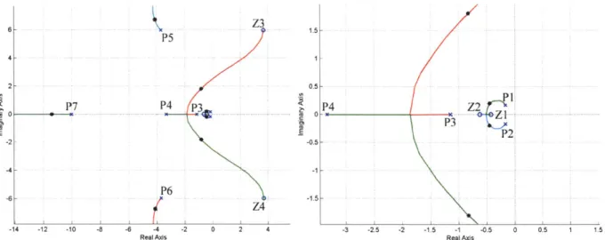
Figure 7.7: Pole-Zero plot for the rudder dynamic model... ₉₃

Figure 7.8: Experiment results for elevator with the ₂nd order model ... ₉₄

Figure 7.9: Experiment results for elevator with the ₂nd order model and time delay... 95

Figure 7.10: Pole-Zero plot for the elevator dynamic model ... ₉₅

Figure 8.1: H eading control diagram ... ₉₇

Figure 8.2: Root Locus for heading system without tailcone dynamics... 98

Figure 8.3: Root Locus plot for the heading system with tailcone dynamics... 99

Figure 8.4: Pitch control diagram ... ₁₀₀

Figure 8.5: Root Locus for pitch system without tailcone dynamics ... 101

Figure 8.6: Root Locus plot for the pitch system with tailcone dynamics ... 102

Figure 8.7: D epth and pitch control diagram ... 102

Figure 8.8: Root Locus plot for the depth-pitch system with tailcone dynamics ... 103

Figure 9.1: Rudder step response mission for commanded angles of -10, 10, -15, and 15 degrees ... 106

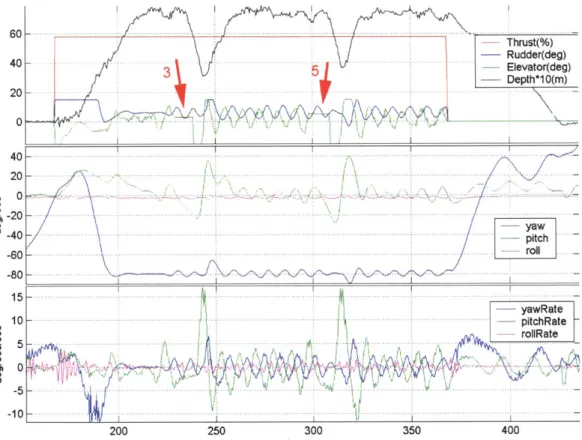
Figure 9.2: Elevator step response mission for commanded angles of 3, and 5 degrees... 107

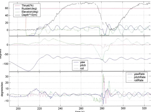
Figure 9.3: Typical usable rudder step response mission ... 108

Figure 9.4: Model adjustment simulation process... ₁₀₈

Figure 9.6: Closed-loop straight run with heuristically tuned controller... 116

Figure 9.7: Yaw model improvements, 10' rudder angle... 117

Figure 9.8: Yaw model improvements, 150 rudder angle... 117

Figure 9.9: Pitch model improvements, 50 elevator angle... 118

Figure 9.10: Pitch model improvements, 15' elevator angle... 118

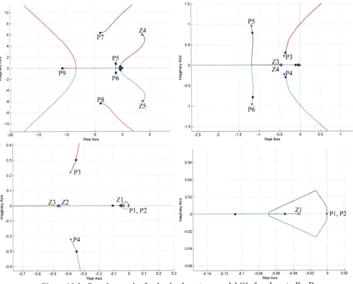
Figure 10.1: Root Locus plot for the heading system, model Cl_5 and controller B ... 122

Figure 10.2: Root Locus plot for the pitch system, model Cl_5 and controller B... 123

Figure 10.3: Root Locus plot for the depth system, model Cl_5 and controller B... 124

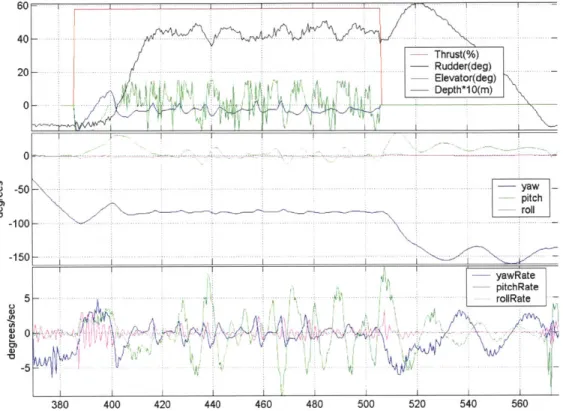
Figure 10.4: Field test at 40%, 60% and 80% thrust with controller B... 125

Figure 11.1: Desired rudder and actual rudder simulation responses... 128

Figure 11.2: Simulation straight run with rudder correction problem... 129

Figure 11.3: Controlled straight run at 4m depth and -80' heading, controller Al... 130

Figure 11.4: Controlled straight run at 3m depth and -80' heading, controller B... 130

Figure 11.5: Controlled heading change from -80' to -60' to -80' at 4m depth, controller Al... 131

Figure 11.6: Controlled heading change from -80' to -60' to -80' at 4m depth, controller B... 131

Figure 11.7: Controlled depth change from 4m to 5m to 4m at -80' heading, controller Al... 132

Figure 11.8: Controlled depth change from 4m to 5m to 4m at -80' heading, controller B... 132

Figure 11.9: Controlled coupled heading and depth change, controller B ... 133

Figure 11.10: Controlled shallow run at im depth and -80' heading, controller B... 134

Figure B. 1: Root Locus plot for the heading system, model A and controller Al ... 141

Figure B.2: Root Locus plot for the heading system, model A and controller Al ... 142

Figure B.3: Root Locus plot for the heading system, model A and controller Al ... 142

Figure B.4: Root Locus plot for the heading system, model B and controller Al ... 143

Figure B.5: Root Locus plot for the pitch system, model B and controller Al ... 144

Figure B.6: Root Locus plot for the depth system, model B and controller Al ... 145

Figure B.7: Root Locus plot for the heading system, model B and controller B... 146

Figure B.8: Root Locus plot for the pitch system, model B and controller B ... 147

Figure B.9: Root Locus plot for the depth system, model B and controller B ... 148

Figure B. 10: Root Locus plot for the heading system, model C1_5 and controller A1 ... 149

Figure B. 11: Root Locus plot for the pitch system, model Cl_5 and controller Al ... 150

Figure B. 12: Root Locus plot for the depth system, model Cl_5 and controller Al ... 151

Figure B. 13: Root Locus plot for the pitch system, model C1_5 and controller A2... 152

Figure B. 14: Root Locus plot for the depth system, model Cl 5 and controller A2 ... 153

Figure B.15: Root Locus plot for the heading system, model Cl_5 and controller B... 154

Figure B.16: Root Locus plot for the pitch system, model Cl_5 and controller B ... 155

Figure B. 17: Root Locus plot for the depth system, model C1 5 and controller B ... 156

Figure B. 18: Root Locus plot for the heading system, model C2_0 and controller B... 157

Figure B. 19: Root Locus plot for the pitch system, model C2_0 and controller B ... 158

List of Tables

Table 2.1: Odyssey III class specifications (Bluefin Robotics Corp.)... 20

Table 2.2: Center of mass and volume with respect to body-frame origin... 22

Table 2.3: Inertial properties with respect to body-frame origin ... 22

Table 3.1: Variables used in duct thruster angle analysis... 27

Table 4.1: Axial added mass parameter cx [18]... 37

Table 4.2: Short Caribou configuration non-linear force coefficients... 45

Table 4.3: Short Caribou configuration non-linear moment coefficients ... 46

Table 4.4: Extended (1.05m) Caribou configuration non-linear force coefficients... 47

Table 4.5: Extended (1.05m) Caribou configuration non-linear moment coefficients... 48

Table 5.1: Short Caribou configuration linear force coefficients, U=1.5m/s ... 61

Table 5.2: Short Caribou configuration linear moment coefficients, U=1.5m/s ... 62

Table 5.3: Extended (1.05m) Caribou configuration linear force coefficients, U=1.5m/s ... 63

Table 5.4: Extended (1.05m) Caribou configuration linear moment coefficients, U=1.5m/s ... 64

Table 5.5: Extended (1.05m) Caribou configuration linear force coefficients, U=1.3m/s ... 65

Table 5.6: Extended (1.05m) Caribou configuration linear moment coefficients, U=1.3m/s ... 66

Table 5.7: Short Caribou configuration linear force coefficients, U=1.5m/s ... 72

Table 5.8: Short Caribou configuration linear moment coefficients, U=1.5m/s ... 73

Table 5.9: Extended (1.05m) Caribou configuration linear force coefficients, U=1.5m/s ... 74

Table 5.10: Extended (1.05m) Caribou configuration linear moment coefficients, U=1.5m/s ... 75

Table 5.11: Extended (1.05m) Caribou configuration linear force coefficients, U=1.3m/s ... 76

Table 5.12: Extended (1.05m) Caribou configuration linear moment coefficients, U=1.3m/s ... 77

Table 8.1: Initial controller gains based on the initial model ... 104

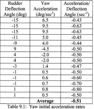
Table 9.1: Y aw initial acceleration rates ... 110

Table 9.2: Pitch initial acceleration rates... 110

Table 9.3: Original and adjusted models A, B, and C ... 111

Table 9.4: Yaw plane model information... 112

Table 9.5: Pitch plane model information ... 112

Table 9.6: Rate error squared sensitivity to parameter changes ... 113

T able 9.7: Stability indicators... 114

T able 9.8: T urning rates and radii... 115

Table 9.9: Pitch plane transfer functions ... 115

T able 9.10: M odel im provem ents... 116

Table 10.1: Controller gains used in the field... 119

Table 10.2: Closed loop poles for model A, model B and model C ... 120

Chapter 1

Introduction

1.1

Background

Developments made in autonomous underwater vehicle (AUV) related technologies have enabled AUVs to move out of the research laboratory and into commercial, military, and scientific areas.

The commercial use of AUVs centers on the gas and oil industry. The Hugin AUV, developed by Kongsberg Simrad, is used by C & C Technologies as its workhorse for high-resolution seabed mapping and imaging for commercial mapping and oil pipeline surveying. The Racal Survey Group Ltd plans to use Bluefin AUVs for shallow and deep water surveys for the oil and gas industry, as well as cable inspection, dredging, and alluvial mining.

Military use of AUVs focuses on surveillance, minesweeping and mine countermeasure work. Lockheed Martin Corp. has developed a Remote Minehunting System (RMS) for surveillance, minesweeping and reconnaissance. The CETUSTM AUV, whose prototype was developed by the MIT

Sea Grant AUV lab, has also been used by Lockheed Martin for mine countermeasures. The Naval Postgraduate School in Monteray, CA, works with a focus on clandestine mine countermeasures, using the ARIES AUV. The Naval Oceanographic Office AUV Program, which started with a large AUV developed and tested at Draper Labs, has focused efforts on multiplying the effectiveness of oceanographic survey ships, by allowing survey of larger areas in less time than with the ship alone.

The scientific community continues to make advancements in AUV usage. MBARI uses AUVs and ROVs for high-resolution mapping of the deep ocean floor, as well as mapping salinity, temperature, oxygen, fluorescence, backscatter and pH over a full annual cycle. MBARI has also teamed with MIT and several other partners to develop an AUV for Arctic research. This Atlantic Layer Tracking Experiment (ALTEX) plans to reach unprecedented endurance and the ability to relay data through ice to satellite receivers. Quantitative survey of hydrothermal plumes and other near-bottom surveys in rugged seafloor terrain have been completed by the Woods Hole Oceanographic Institution, using the ABE vehicle. The Alfred Wegener Institute for Polar and Marine Research has planned a 4-D mapping of a methane plume above a cold seep at the Norwegian continental margin. The REMUS vehicle, operated at Woods Hole, as well as Ocean Explorer, operated at Florida Atlantic University, have both demonstrated the capability to dock autonomously with a base station. These scientific and research pursuits demonstrate that the usage and capabilities of AUVs are continuing to grow.

1.2

Motivation

Continual improvement in all areas of the performance of autonomous underwater vehicles (AUVs) is needed to enhance the developments made in long-range oceanographic surveys, shallow-water mine reconnaissance and countermeasures, and procedures in autonomous docking as well as other tasks [1]. One aspect of this performance improvement is maneuvering, which can be achieved by improving the vehicle's control system. In order to develop a precise control system, a good controls platform is needed for testing and research purposes. In this case, that platform is a finely tuned dynamic model of the vehicle. Previous work in dynamic modeling of AUVs includes simulation model verification done through field tests [2] as well as theoretical and empirical methods in addition to tow tank results [3]. Recent work done on AUV control has included gains obtained using partial model matching methods [4], as well as sliding mode control based on estimated coefficients [5], in addition to fuzzy sliding mode control systems [6].

The Odyssey III AUV used for this work is highly maneuverable and has a variable configuration in length and payload. It can operate at a range of speeds, and it has a novel propulsor and control surface that consists of a double-gimbaled ring finned duct thruster, which allows for vectored thrusting. These attributes make the modeling and control of substantial interest and challenge. Odyssey III is also a leading design in current AUVs, so this analysis is extremely relevant. The dynamic simulation modeling and control of the Odyssey III AUV through system identification tests is addressed in this work. Previous work in system identification of AUNV systems has been done using neural network identifiers

[7] and neurofuzzy identification techniques [8]. The work presented here focuses on development of

dynamic models and control systems from first principles. The system identification tests and simulation process form a forward design process.

1.3

Research Platform Caribou

The autonomous underwater vehicle (AUNV) platform for this research was an Odyssey III class vehicle, Caribou. This AUV was built by Bluefin Robotics Corporation, and is one of several AUVs at MIT Sea Grant. Caribou represents the culmination of significant development efforts. Featuring a modular hull design and the latest evolution of AUV navigation, propulsion and power systems, Caribou provides significant new autonomous underwater surveying capabilities and flexibility for various scientific needs. The operating system, which Caribou uses to operate, is called MOOS (Mission Oriented Operating Suite). This operating system is composed of C++ classes and it uses a publish-and-subscribe protocol.

[9]

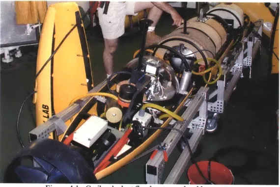
Figure 1.1: The Caribou autonomous underwater vehicle in short configuration

Caribou's modular payload section approach allows a single vehicle to support widely different missions. The short configuration was designed to accommodate the Edgetech(R) FS-AU side-scan sonar and sub-bottom profiler, while additional payload sections can accommodate numerous other scientific packages, as well as additional battery power. Caribou is equipped with state-of-the-art sensors, which allow it to

collect high-quality data. Caribou will be used in the near future by the AUV Lab at MIT Sea Grant for archaeological remote sensing [10], multi-static acoustic modeling [11], fisheries resource studies and development of concurrent mapping and localization techniques [12]. Figure 1.2, shows the process used to develop an accurate model and control system for the AUV, as described in this thesis.

Initial

Model Adjustment

Dynamic

Procedure to fit Model

Model

Responses to the

lILI

AUV Test Responses

Initial

Conservative

Revised

Model

Figure 1.2: System Identification modeling and control procedure

1.4

Simulation Model Development

Described in this thesis is the development and verification of a simulation package for the motion of an autonomous underwater vehicle in six degrees of freedom, or less. This simulation model is used to adjust the model coefficients so that the simulation results closely match the results found from field tests, as shown in Figure 1.2. The external forces and moments resulting from the vehicle hydrostatics, hydrodynamic lift and drag, added mass, and the control input of the vehicle's ducted thruster are all defined in terms of specific coefficients for this model [28]. This thesis describes the derivation of these coefficients in detail. Substantial work was performed in adjusting and verifying these coefficients in order to validate the vehicle's model results with the results from field experiments with the vehicle.

Nonlinear equations were used to determine the vehicle's coefficients, and rigid-body dynamics.

A linearized model was also derived and the simulation has the capability of using either model. While

the vehicle is inherently nonlinear, the nonlinear simulations provide more realistic simulations, but for control purposes, the linear model provides a sufficient platform, while maintaining less complexity. The simulation package operates on the numeric integration of the equations of motion, using Matlab integration software. The simulation output was checked with various data collected from field experiments. The simulator was shown to not only accurately model the vehicle motion in six degrees of freedom, but also in the independent three degrees of freedom yaw plane and pitch plane, due to the decoupled nature of the system.

In order to simplify the challenge of completely modeling an autonomous underwater vehicle, it was necessary to make several key assumptions on which to base the simulation model development. The following assumptions about the vehicle and the environment were made:

* The vehicle is a rigid body of constant mass, i.e. the vehicle mass and mass-distribution does not change during operation.

" _{The vehicle is deeply submerged in a homogenous, unbounded fluid, that is, the vehicle is} located far from the free surface (no surface effects, i.e. no sea waves or vehicle wave-making loads), walls, and bottom.

* _{The vehicle does not experience memory effects, i.e. the simulator neglects the effects of the} vehicle passing through its own wake.

* The vehicle does not experience underwater turbulence

1.5

System Identification

System identification tests were performed in the field to help fit the model response to the responses seen in the field, by adjusting model coefficients and parameters, as shown in Figure 1.2. This allows a more precise controller to be designed as the dynamic model is adjusted to more closely model the AUV. The system identification tests used were simple step response tests. The AUV was roughly controlled to a desired depth and heading angle using a controller that was designed from the original dynamic model. At this controlled state, the heading controller was turned off, and the rudder was commanded to a desired deflection angle for a short response time. Likewise, the pitch plane system was examined by turning the depth and pitch controllers off and setting the elevator to a prescribed angle for a short response time. During the rudder step tests, the pitch and depth controllers were left on, and during the elevator step tests, the heading controller was left on. These simple step response test results were then used to adjust the dynamic model coefficients and parameters. This approach proved to worked well and resulted in a much more accurate dynamic model, and a much improved control system.

1.6

Controller Development

The controller development described in this thesis is based heavily on experimentally obtained data that was used to drive system identification, as outlined in Figure 1.2. Based on an initial linear model of the

AUV, a conservative initial controller was developed using Root Locus methods. This controller was

then used to perform a very compact set of system identification tests designed to identify the vehicle dynamic response. Using the data from these tests, the dynamic model was improved, and a revised, precision controller was developed based on this updated model. This precision controller showed significant improvements when used during closed-loop maneuvers, as compared to the same tests done with the initial controller as shown in Chapter 11. This work shows that the simple, forward design from basic principles allowed us to design an accurate control system without spending more than a few hours in the water.

1.7

Thesis Outline

The discussion of this work begins with a closer looks at the AUV, Caribou, and then moves on to the equations of motion, the nonlinear coefficients as well as the linearized models and the vehicle simulation. The testing and modeling of the tailcone system is presented next, followed by the initial controller design. Then the system identification process is addressed as well as the redesign of the control system. Finally, the results of field tests using the initial controller and the redesigned controller are explained as well as the conclusions and future work to be addressed.

Chapter 2

The Odyssey III Class AUV Caribou

Prior to calculating the hydrodynamic and hydrostatic coefficients of the vehicle, several characteristics of the vehicle needed to be determined: vehicle hull profile, mass distribution, and buoyancy properties.

2.1

Vehicle Profile

The hull shape of the Odyssey III vehicle is based on a Series 58, Model 4154 Gertler polynomial [13] defined below, with a length of 84in (2.13m) and a maximum diameter of 21in (0.53m). The origin of this polynomial is at the nose of the vehicle, with the x-axis along the horizontal plane of the vehicle. The y-axis is in the vertical plane, and describes the radial magnitude at the corresponding position on the x-axis as shown in Figure 2.1.

y2 = alx+ a2x2 + a₃x3 + a4x4 + a5x5 + a6x6 (2.1) where a, =+ 1.000000 a2 =+ 2.1496653 a₃ = - 17.773496 a4 =+36.716580 a5 = - 33.511285 a6 =+11.418548 and x = (2.2) L

Therefore, x is a non-dimensional ratio of position X with respect to L, where L is the total length of the streamlined vehicle (i.e. 2.13m) and X is the longitudinal position from the nose of the vehicle.

to

x

Y

Figure 2.1: Profile of Caribou's prescribed shape

2.2

Caribou Specifications

The Odyssey III Class AUV was designed with a modular approach in mind. This means that additional payload sections could be added to the mid-section of the vehicle for various mission tasks. As prescribed by the hull profile in section 2.1, the maximum radius of 0.267m occurs at a point, x=0.40 from the vehicle nose using the Gertler equation. For the nominal hull length of 2.13m (84in), this point is at 0.884m from the nose. Caribou's short configuration (i.e. without additional payloads), includes a standard mid-body extension of 0.377m, for an overall streamlined body length of 2.51 lm. With the addition of the ring fin, the standard body length is 2.58m. Additional cylindrical payload sections can be added. A typical payload is approximately lm in length and 0.58m in diameter.

These additional payloads, of course, alter not only the physical specifications of the vehicle, but also the vehicle coefficients, inertial terms and control capabilities. Table 2.1 below lists parameters for the short configuration, i.e. no additional payloads.

Vehicle Configuration Length:

Maximum Diameter: Mass in air:

Mass in water:

Short Base Vehicle

2.58 m (102 inches)

-250 kg (550 lbs)

-400 kg (880 lbs)

Extended Vehicle for Tests

3.63 m (144 inches) 0.533 m (21 inches) -350 kg (770 lbs) -650 kg (1400 lbs) Buoyancy: Maximum Depth: Operation Depth: Survey Speed: Survey Endurance: Batteries: Line Keeping: Altitude Keeping: Payload: -+2.2 kg (+51bs.) 4500 m 3000 m 3-4 knots (1.5-2 m/s) 20 hours (at 3 knots)

Lithium Polymer 2 meters

1 meter

Designed to accommodate various sonar, oceanographic systems in modular sections.

Table 2.1: Odyssey III class specifications (Bluefin Robotics Corp.) camera, and

2.3

Ring Fin Propeller

The Caribou vehicle is equipped with a double-gimbaled vector duct thruster. The duct thruster's angle is limited at ±15degrees in both the yaw and pitch plane, known typically as the rudder and elevator angle. The propeller is confined to the duct for protection, as well as enhanced flow capabilities. The duct also acts as a control surface. Thus, the Odyssey III class AUV does not need control fins to control the vehicle motion because the duct and vector thrusting capability is sufficient to impose directional control. Figure 2.2 shows the duct thruster arrangement.

Figure 2.2: Ring fin duct thruster arrangement on Caribou

2.4

Coordinate Systems

For this work, the body referenced coordinate frame is located along the symmetric axis of rotation at the midpoint of the AUV. In this body coordinate system the x-axis is along the symmetric line proceeding towards the nose of the vehicle. The y-axis extends towards the port side of the AUV, while the z-axis is directed upwards (Figure 2.3). Body referenced velocity in the x direction, surge, is denoted by u. Velocity in the body frame y and z directions is v, sway, and w, heave, respectively. Rotational velocity about the x-axis, roll velocity, is denoted as p. Rotational velocity about the y-axis and z-axis is q, pitch rate, and r, yaw rate, respectively. External body forces in the x, y and z direction are denoted as X, Y and Z respectively, while external body moments in the x, y and z direction are K, M and N respectively. The vehicle's angular orientation is described in the inertial frame of reference with Euler angles, W, 0, and >, as described in Section 3.2.

Inertial-frame

coordinate system _{SURGE: u, X}

QLD

Body coordina HEAVE: w, Z YAW: r, N

-+5*

2.5

Vehicle Weight and Buoyancy

The buoyancy force of Caribou depends strictly on the hull's geometry and is simply the weight of the vehicle's displaced volume of water. For each separate hull configuration, this value stays fixed, because there are no major changes in the vehicle's hull. However, the mass of the Caribou vehicle can change between missions, depending on the type of batteries used in the vehicle, the electronics devices used, and the amount of ballast added. The Caribou vehicle is typically ballasted with -2.2 kg (-5 lbs) of positive buoyancy, so that in the event of power or computer failure, the AUV would eventually float to the surface. Integration over the volume of the vehicle, and multiplication by the density of water and acceleration of gravity determined the vehicle's buoyancy force, FB. The vehicle mass was then assumed to be -2.2 kg (-22 N) less than the acting mass of the buoyancy. This value changes slightly during each mission as the vehicle components change, however, the AUV is usually ballasted around +5 lbs buoyant.

2.6

Centers of Buoyancy and Gravity

For each separate hull configuration, the center of buoyancy stays fixed, however, the vehicle center of mass can vary, as between missions it can be necessary to change the vehicle battery packs and re-ballast the vehicle, in addition to changing payloads.

For this work, the origin of the body-coordinate frame is the symmetric middle of the vehicle. The typical parameters for application points of the buoyancy force (center of volume, CV) and vehicle weight (center of mass, CM) are shown in Table 2.2 for the short vehicle configuration, with respect to the body-frame origin. The position of the center of volume and center of mass along the x-axis are usually about the same and the center of volume and mass along the y-axis is generally zero as the AUV is generally ballasted to achieve zero static pitch and roll. Like the buoyancy force, these parameters can vary from mission to mission because the vehicle configuration changes.

Parameter Value Units

XCM 8.2 Cm YCM 0.0 cm ZCM -2.1 cm XCV 8.2 cm Ycv 0.0 cm ZCV

0.0

Table 2.2: Center of mass and volume with respect to body-frame origin

2.7

Inertia Tensor

The vehicle inertia tensor is defined with respect to the body-frame origin at the vehicle's symmetric mid-section. As the products of inertia Iy, Ixz, and IYZ are small compared to the moments of inertia Ixx, Iyy, and Izz, and assuming that the vehicle has two axial planes of symmetry, we will assume that they are zero.

The inertial values were estimated based on the integration of a homogenous vehicle hull with an average density of that of water. The estimated values are given in Table 2.3 for the short vehicle configuration.

Parameter Value Units

IXX 12 kg-m2

Iyy 133 kg-m2

Izz 133 kg-m2

Chapter 3

Governing Equations of Motion

In Chapter 3 the kinematics, dynamics, and mechanics of the Odyssey III vehicle and simulation model are defined and explained. These derivations contribute to the initial dynamic model, which is the first

step in the controller design process as outlined in Figure 1.2.

3.1

Body-Frame Coordinate System

All future calculations in this text will regard the body-frame coordinate system origin to exist at the

vehicle's symmetric midpoint as explained in Section 2.4 and illustrated in Figure 2.3.

3.2

Vehicle Kinematics

The vector transformation from an inertial frame of reference to the body frame is as shown below. The transformation is developed by using Euler angles (y,O,4), which describe the roll, pitch and yaw position of the vehicle in inertial space. Roll, pitch and yaw are the rotations of the body about the x, y, and z-axes, respectively. The transformation R(y,O,4) was calculated by cascading the 3 separate angular transformation matrices. The order of the rotations from the inertial frame of reference was: rotation about the z-axis with the yaw angle

4,

cOCO c Os 0 -so]

XB

-Cqk0sV~S0cq0

c

Vgcq5+sy/s Osb

0

sy/cO

XI

=R(y',O,q0)Xj

(3.1)

sXB s#+[Cqs0C# -syc+cVysOs# c yco]

The transformation matrix R(y, 0,

4)

The motion of the body-referenced frame is described relative to an inertial frame of reference. The general motion of the vehicle in six degrees of freedom is described by the following twelve states.

x S=y

Lz]

position of the body origin in inertial space _(3.3)

Euler angles with respect to inertial space _(3.4)

the body-referenced translation velocities _(3.5)

the body-referenced rotational velocities (3.6)

A vector can be used

inertial space.

to represent the Euler angles that determine the roll, pitch and yaw position in

S=0

FV0-

For the case of infinitesimal Euler angles, the time rate of change of these Euler angles is equal to the body-referenced rotation rate, @3, however, for larger Euler angles the physically determined rotation rate, & , needs to be related to the time rate of change of the Euler angles as follows [14].

1 0

-so

W = 0 c sqic

Z=F-'(Z)Z=

0 -sV cVcO r.

(3.8)

The derivatives of the body velocity, i;, and rotation rate, >, come from the equations in Section 3.3 for the external forces and moments [X,Y,Z] and [K,M,N]. The derivatives for . and £ come from the following relationships.

. = R (x, ,#)_ (3.9)

The vector & is the vector containing roll, pitch, and yaw rates: p, q, and r respectively. The inverse of the transformation matrix F' (F) provides the following relationship [14].

E=

_0 sVC c V yIc_c

Equations 3.9 and 3.10 provide a relationship between measurable quantities that are readily available, and the variables that need defining. Note that F(E) is not defined for pitch angles at 0= ±900. This is not a problem, as the vehicle motion does not ordinarily approach that singularity. If this situation were to occur, then it would become necessary to model the vehicle motion through extreme pitch angles, and the analysis could then resort to an alternate kinematics representation such as quatermions.

3.3

Vehicle Rigid-Body Dynamics

The locations of the vehicle centers of mass and volume (buoyancy) are defined in terms of the body-fixed coordinate system as follows. The values for the center of mass and volume are shown in Table 2.2.

XCM CV

XB= C VJ _(3.11)

SB

O

ZCM

ZCV

The vessel inertial dynamics were derived from the physics of the system and are written as follows in the body-referenced frame. With xcM, _{ycM, and ZCM defining the location of the vessel's center of mass with}

respect to the body-referenced coordinate frame origin. X, Y and Z are the external body forces applied in the body-referenced directions of x, y and z respectively, as shown in equation 3.12-3.14 [14].

X =mz +qw-rv+4zCM -- yCM C CM p -(q2 +r2)XCM

Y =m[,>+ru - pw+xCM- zCM (rzCM CM 2 CM

Z =m [+ pv -quy+

_PyCM-x

+q2 )zCM

The angular dynamics were derived in a similar way. The body-referenced angular equations of motion also include translation and rotational accelerations as well as velocities.

K = I _{+ I,4 + Ix + (Iz -I,,)rq+I,(q}2 _-r

2)+J pq -Ipr (3.15)

+ m[ycM

(*

M = I, + I,,4+ IJ + (I -

Izz)pr

_ p 2)+ - Iqp (3.16)

+ m[zCM (zi + qw - rv) - XGM (v + pv -

qu)]

N =IJp + Iz,4+Iz + (I,, -Ix)pq +I,, (p2

_

q

) + Ipr - Ixqr (3.17)

+ m[xCM (i + ru - pw) - YCM (zi + qw - rv)]

The equations (3.12-3.17) describe how the AUV will respond to external forces and moments acting in each degree of freedom. These are nonlinear, coupled equations of motion.

3.4

Vehicle Mechanics

Given the body-referenced coordinate system, and assuming a symmetric homogeneous body, the angular inertial properties can be described by a diagonal inertia tensor.

IXX 0 0

I= 0 I,, 0 (3.18)

-0 0 IZZ

Caribou's volume due to the short configuration's prescribed hull shape is 0.394m3. This corresponds to the mass of 394kg in fresh water. The wetted surface area, A,, is 3.378m2_{. The frontal area, Af, is}

1. 14m2. The moments of inertia were computed as follows, treating the vehicle as a homogeneous body

with the density of water. For the short configuration with parameters listed, the standard inertial integration about the center of the body, /2, provided the following with the cross-terms nearly equal to zero for the nearly symmetric vehicle.

Ixx =12 kg-m 2

(3.19)

IY, = IZZ =133 kg -m2

For the extended hull AUV, the moments of inertia and added mass change. Adding the cylindrical term increases the moment of inertia in the x-axis. Adding not only the cylindrical term, but also a term corresponding to the parallel axis theorem for the extended original configuration increases the moment of inertia in the y-axis and z-axis.

=

J-2pcrdx

2

I=

p7r

(3r

+h2

2 LI

The result of the combined external forces and moments is described as follows:

X'

Y [ B,bodylift +B,bodydrag ±FB,tailcone + FB,thrust +FB,hydrostatics + B,crossterms] (3.22)

Z

K

M = f B,bodylift +MB,bodydrag +MB,tailcone + B,thrust B,hydrostatics B,crossterms] (3.23)

TNd

3.5

_{The Double-Gimbaled Duct Thruster}

The tailcone of the Caribou AUV is a double-gimbaled duct thruster. The deflection angle of this duct is a combination of the yaw rotation, known as the rudder angle, and the pitch rotation, known as the elevator angle, due to the double-gimbaled arrangement. Rotational transformations were developed to relate the position of the duct to the body frame coordinate system. Table 3.1 notes the nomenclature used in this development.

T_ _Thrust

dE=8e _{Commanded elevator angle in the body frame}

dR=8r Commanded rudder angle in the body frame dEdesired=6edesired _{Desired elevator angle in the inertial frame} dRdesired=8rdesired _{Desired rudder angle in the inertial frame}

W Roll angle in the body frame

Table 3.1: Variables used in duct thruster angle analysis

The tailcone is double gimbaled; therefore there are several transformations that need to be addressed

(Figure 3.1). Z2 dR ZB z' dE X( dE Xi _dR X2 YB dE f y2

Figure 3.1: Body frame, elevator frame and rudder frame

The commanded elevator actuation is done relative to the hull, while the commanded rudder actuation is performed relative to the elevator position. Hence, the first rotation is made about the y-axis in body coordinates. This rotation is the commanded elevator angle of rotation. This new coordinate system (1) can be related to the body coordinate system (B) as follows:

x

I

_-snie

yI =YB (3-24

The second rotation is made about the z-axis in the (1) frame of reference. This rotation is the commanded rudder angle of rotation. This new coordinate system (2) can be related to the coordinate system in frame (1) as follows:

x2 = cos(, )x, _{+ sin(3, )y}

Y2 = cos(0, )yj - sin(5, )xl (3.25)

Z₂ =Z

The thrust from the propeller is always in the negative x direction of the (2) frame and therefore may be written as follows.

Frrust

-- Tx

Combining the results of equations 3.24 and 3.25 with equation 3.26, the following relationship is established in body coordinates.

FTrust =-TPx2

- -Tp cos(3r )xI - Tp sin(5r )y(

- -Tp COS(Sr )[cos(5e )XB - sin(de )ZB

Tp

= -T, [cos(5r) cos(5,)XB + sinQ5r )YB cos(5r

)

cos(,r

)

Frust =-T, sin(S) = (3.28)

-cos(,.

₎

Equation 3.28 shows that the magnitude of the thrust force in the body frame directions depends upon both the commanded elevator and rudder angle. From this equation, the imposed rudder deflection in the body frame is tan-1(-Fy/-Fx) and the imposed elevator deflection in the body frame is tan-1_(Fz/-Fx). Therefore from equation 3.28, the imposed rudder deflection in the body frame is tan-'[tan(6r)cos(6e)], while the imposed elevator deflection in the body frame is 6e. Thus, the imposed elevator angle is decoupled from the commanded rudder angle, but the imposed rudder angle in the body frame is dependent upon both the commanded rudder and commanded elevator angles. This is because the commanded rudder deflection is made relative to the elevator frame in the double-gimbaled duct thruster arrangement.

However, if the commanded elevator angle is small, which it is set to be less than 15 degrees, then the imposed rudder deflection and imposed elevator deflection are approximately the commanded angles 6r and 6, respectively. The vehicle is modeled using this assumption, and the heading and pitch/depth control are assumed to be done in a frame that is not affected by vehicle roll. This assumption is made because the roll of the vehicle is generally small due to the large righting moment. This is how Caribou's control system operated in the field for this work.

3.6

Duct Angle due to Vehicle Roll

The development in Section 3.5 does not take into account the roll of the vehicle. Generally this roll angle is small; however, a more accurate control system may take this roll angle into account. When the

AUV rolls, a body referenced rudder deflection is not the same as an inertial referenced rudder deflection.

The same is true for the elevator angle. Therefore, in order to achieve a desired rudder or elevator deflection in the inertial frame, a transformation that relates the desired inertial deflection with the commanded deflection is needed. For this derivation we assume that the thrust, Tp, is constant and acts

along the x2-axis. The vehicle rolls about the x-axis in body coordinates, shown in Figure 3.2. Again, a

transformation can be found that relates this rolling body position to the fixed inertial frame (I).

XB = _I YB Icos(y)Y + sin(y)Z, _(3.29) ZB =cos()Z, _{- sin(V)Y} ZB Zi XB X1 I Y1

Figure 3.2: Vehicle roll with respect to the body frame

Combining the results of 3.27 and 3.29, the following relationship is established that relates the roll angle as well as the commanded rudder and elevator positions to the thrust vector in inertial space (I).

FT,.ust = -T,

[cos(r

cos(6,r

=-T,

{cos(Sr,

)

)[cos(y)Y

)[cos(

or)Z,

]}

-(cos(r)cos(Se))

Fx

FI,,rust =T, -(sin(3r)cos(y))-(cos(3r)sin(S,)sin(y)) _{= Fr (3.30)}

-(sin()5r)sin(ig))+(cos(5r)sin(,)cos(t))j

_LFz

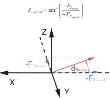
Equation 3.30 shows that the thrust vector, in inertial space is determined by the commanded rudder, commanded elevator and roll angles, as well as the thrust magnitude, Tp. From this equation, the imposed rudder deflection in the inertial frame is tan-'(-Fy/-Fx) and the imposed elevator deflection in the inertial frame is tan-'(Fz/-Fx). Therefore, in order to create a desired rudder deflection in the inertial frame, a desired force along the inertial X and Y axes is needed as shown in Figure 3.3.

(3.31)

(rdesired

tan-'

I

-. F dsre

\Y

d

X

Figure 3.3: Desired rudder position in the inertial frame

Now using the results from 3.30 in equation 3.31 the following relationship is attained, which reduces to equation 3.33. Notice that the thrust, Tp drops out from the equations, and thus has no bearing on the results.

tan(r desired) = FYdered

sin(S,) cos(V)

- F

cos(r)

)

( )tan(Sr )cos(ig)

tan(gr desired - r

COS()

COS(5e)

(3.32)

(3.33)

Likewise, in order to create a desired elevator deflection in the inertial frame, a desired force along the inertial X and Z axes is needed as shown in Figure 3.4. Here equation 3.30 and 3.34 are combined to form equation 3.35 which leads to equation 3.36.

\

desiredF=

tan

tan(Se

_

de

dered

-

sin(5r)sin(V/)

+

cos(3,)sin(e)cos(V)

cos(r

)

cos(Se)

(

)

- tan(S3

)

tan()s

a e desired !

cos(e

(3.35)

z

d

X

-FxJ,.

-Y

Figure 3.4: Desired elevator position

Now the results of equation 3.33 and 3.36 are combined in matrix form to show the following relationship. The desired rudder and elevator angle are the deflection angles of the duct thruster that are desired in the inertial frame. These desired angles are achieved by setting the commanded rudder and elevator angles according to the relationship shown in equation 3.37, which depends also on the roll angle.

tan(Fedesired -cos a -sin

tan(e)

(337)

tan(6,sied, ) _sin]

V

cos

tan(r)/cos(8,)

Equation 3.37 is now arranged so that the commanded rudder and elevator angles are a function of the roll angle and the desired rudder and elevator inertial frame deflection angles.

tan(Se) ~cos Vf - sin V tan(e desired

tan(Sr)/cos(,)j = sin cos y tan(gr desired (3.38)

Equation 3.38 leads to equation 3.39 by inverting the roll transformation matrix.

tan( _{cos y sin V ~tan(e desired)}

Ltan(5,I/cos(e

Finally, reduction from matrix form to equation form provides these results for the commanded deflection angles based on the desired deflection angles in the inertial frame and the roll angle of the AUV. Equation 3.40 represents the algorithm that could be used by the AUV's control system, where the desired rudder and elevator angles in the inertial frame are determined by the controller gains. Then based on these desired inertial angles and the vehicle's roll angle, the commanded elevator and rudder angles are determined. This would provide a more precise approach to the control of the AUV. However, the roll angle and the deflection angles are generally small, which show that under this assumption, equation 3.40 becomes 3.41.

45e = tan [cos tan(edesired

)+

4, = tan- {cos te

-

The one subtlety shown in equation 3.40 is that the desired rudder angle is related to the commanded elevator angle. As was noted earlier, the elevator moves relative to the hull, while the rudder moves relative to the elevator. The cosine term has been carried through the algebra and shows up precisely as

expected in the commanded rudder equation. If the roll angle is assumed to be small, then equation 3.40 becomes 3.41, where the commanded elevator angle is same as the desired elevator angle in the inertial frame and the commanded rudder angle depends on the commanded elevator angle and the desired rudder angle in the inertial frame. This is the same as the derivation made in Section 3.5.

e e desired

r= tan [tan(r desired )cos 5e (3.41)

As was mentioned in Section 3.5, if the commanded elevator angle is small, as it is, then the commanded elevator and rudder angle will be the same as the desired elevator and rudder angles in the inertial frame, again assuming that the roll angle of the vehicle is small.

Chapter 4

Derivation of Nonlinear Coefficients

In this chapter, the coefficients defining the external forces and moments on the vehicle are defined. The vehicle and fluid parameters necessary for calculating each coefficient are included in the section describing the coefficient. This nonlinear model leads to the linearized initial model that is the first step in the controller design process as shown in Figure 1.2.

4.1

Hydrostatics

The vehicle experiences hydrostatic forces and moments as a result of the combined effects of the vehicle weight and buoyancy. The mass and weight of the vehicle is m and W, respectively, where W = mg .The vehicle buoyancy is expressed as B = pVg, where p is the density of the surrounding fluid and V the total volume of water displaced by the vehicle. The buoyancy force acts at the center of volume and the weight act at the center of mass. These positions are expressed in terms of body-frame coordinates.

XCM _CV

fkCM

X

_C

VI

_(4.1)

B$ __ CM B YCV

ZCM _CV

Since the volumetric center and mass center do not coincide in the vehicle, there will be a righting moment that is induced whenever the vehicle is rotated from its stable position. The position vector for the vehicle's center of mass is X7c defined relative to the body frame origin. The position vector for the vehicle's volumetric center is X7v, again in body frame coordinates described from the body origin. Using the previously defined rotational transformation matrix, R(, 0, ) from equation 3.1, the weight and buoyancy forces can be transformed from the inertial frame to the body frame.

.i0 = 0

FB,,eight = R(yf,0,#) 0 FBbyny = R(Vf, 0,#0) 0 (4.2)