Dynamic Reconstruction
The MIT Faculty has made this article openly available.
Please share
how this access benefits you. Your story matters.
Citation
Horn, Berthold K. P. et al. “Dynamic Reconstruction.” IEEE
Transactions on Nuclear Science 57.1 (2010): 193–205. © Copyright
2010 IEEE
As Published
http://dx.doi.org/10.1109/tns.2009.2032544
Publisher
Institute of Electrical and Electronics Engineers (IEEE)
Version
Final published version
Citable link
http://hdl.handle.net/1721.1/73043
Terms of Use
Article is made available in accordance with the publisher's
policy and may be subject to US copyright law. Please refer to the
publisher's site for terms of use.
Dynamic Reconstruction
Berthold K. P. Horn, Richard C. Lanza, Jayna T. Bell, and Gordon E. Kohse
Abstract—Dynamic reconstruction is a method for generating
images or image sequences from data obtained using moving ra-diation detection systems. While coded apertures are used as ex-amples of the underlying information collection modality, the dy-namic reconstruction method itself is more widely applicable. Dy-namic reconstruction provides for recovery of depth, and has sen-sitivity that drops off with the inverse of distance rather than the inverse square of distance. Examples of dynamic reconstructions of moving isotopic area sources are shown, as well as dynamic recon-structions of moving objects imaged using backscattered X-rays.
Index Terms—Back projection, coded apertures, computational
imaging, dynamic reconstruction, moving detector systems, tomo-graphic reconstruction, X-ray backscatter.
I. BACKGROUND
D
YNAMIC reconstruction forms images computationally from data obtained by moving radiation detector systems. It is related to coded aperture imaging and computerized tomog-raphy and borrows ideas from both.A. Coded Aperture Imaging
Static coded apertures have been used for imaging with radia-tion that cannot be refracted or reflected – such as (hard) X-rays, gamma rays and neutrons [1]–[7]. Lenses and mirrors are ruled out for image formation when refraction and reflection are not possible or not practical. While pinholes and collimators can be used in these circumstances, these have a poor tradeoff between sensitivity and resolution [8], [9].
Coded aperture imaging masks are made of materials that are (more or less) opaque to the radiation of interest, with holes in carefully selected positions. If the mask is parallel to the de-tector plane, then the shadow cast on the dede-tector resulting from a point source is an enlarged and shifted version of the mask pat-tern itself. The mask patpat-terns chosen typically have the bilevel autocorrelation property, that is, the (cyclical) autocorrelation of the pattern can take on only two values, one for zero shift and a unique second value for all other shifts [10]–[12]. Equiv-alently, the power spectrum (magnitude of Fourier transform) is two valued, with one value for zero frequency (DC) and another unique value for all other frequencies [9], [13].
Manuscript received January 13, 2009; revised June 18, 2009. Current version published February 10, 2010.
B. K. P. Horn is with the Department of Electrical Engineering and Computer Science, Massachusetts Institute of Technology, Cambridge, MA 02139 USA (e-mail: [email protected]).
R. C. Lanza and J. T. Bell are with the Department of Nuclear Science and En-gineering, Massachusetts Institute of Technology, Cambridge, MA 02139 USA. G. E. Kohse is with the Nuclear Reactor Laboratory, Massachusetts Institute of Technology, Cambridge, MA 02139 USA.
Color versions of one or more of the figures in this paper are available online at http://ieeexplore.ieee.org.
Digital Object Identifier 10.1109/TNS.2009.2032544
The standard image reconstruction technique for static coded apertures is correlation of the detector output pattern with the (magnified) mask pattern itself (or a pattern obtained by simple transformation of the mask pattern). Correlation may be imple-mented directly or by multiplication in the Fourier transform domain. The main application of coded aperture imaging so far has been in X-ray astronomy [2], [5], [6], [14] and imaging of explosive events, although coded aperture techniques have been applied to other problem areas such biomedical imaging [15].
In X-ray astronomy, the enormous distance to sources pre-cludes any significant effect of translational motion of the de-tector and mask on the image. Further, rotation only induces changes in the way the detector array samples the image. Tradi-tional coded aperture reconstruction techniques in effect assume a fixed geometric relationship between detector, mask and target and so do not apply directly to moving radiation detecting sys-tems where the image changes due to changes in perspective. B. Tomographic Reconstruction
Another relevant technique is tomographic reconstruction [16]. In tomography, relative motion between target and de-tector system is purposefully introduced in order to scan a target area or volume. Each detector receives information about radiation that followed a single line from source to detector. The most popular reconstruction technique for tomographic problems is “filtered backprojection.” Typically, the projection data is first processed using a (one-d) filter, usually a form of “ramp” filter [16]–[18] whose response is proportional to the spatial frequency (up to some limit). This may be implemented directly, using convolution, or in the Fourier transform domain. An alternate, equivalent, approach is to first back-project the projection data (i.e., without prior filtering). The result is the desired image convolved with a point spread function (PSF) proportional to the inverse of radial distance ( ). The image “blur” introduced can be undone by convolving with a (two-d) filter whose transform has magnitude directly proportional to spatial frequency ( ).
Tomographic techniques are widely used in CT, nondestruc-tive testing, microscopic imaging, and MRI [16]. Tomographic reconstruction methods are not restricted to applications of the oft-cited “Fourier-Slice” theorem, which does not apply directly to scanning schemes other than the rarely applicable parallel beam organization [17], [18].
Traditional tomographic reconstruction techniques do not apply to moving coded apertures, because at any given time, the coded aperture mask allows radiation from several different target points to reach a particular point on the detector. So the measured signal is not the integral of some quantity (such as density or activitiy) along a single ray as required for tomo-graphic reconstruction.
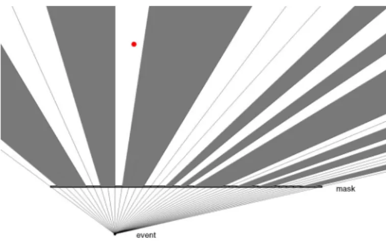
Fig. 1. Projection: radiation from a point in the target volume can reach some areas of the detector through open areas of the mask. Other areas of the detector are shadowed.
C. Scanning Coded Aperture Systems
Thus there is a need for a method that can reconstruct 2-D or 3-D images from data produced by moving radiation detection systems such as coded aperture detector systems. The increased flux available from coded apertures as compared to pinholes or collimators is often needed or desired. Further, relative motion between the detector system and the target may be either un-avoidable, or purposefully introduced in order to scan an area.
II. DYNAMICRECONSTRUCTION
One way to think of the dynamic reconstruction technique is essentially as geometrically guided, weighted “back projec-tion.” The detector data is backprojected onto a target area or target volume based on the current geometric relationship of the detector system and the target.
Algorithm
Back projection may be repeated for every “event” (e.g., photon reaching the detector at a known position). Alterna-tively, radiation flux can be integrated over a short period of time at each detector element of a discrete array and the accumulated “frame” back projected. The algorithm may be motivated by reference to Fig. 1 showing projection onto the detector system and Fig. 2 showing back projection onto an accumulator array representing the target area.
In particular implementations, the target area or volume may be represented using a 2-D or 3-D array of accumulator cells (pixels or voxels), each corresponding to a defined position in space (or a small area or volume). Each event is “backprojected” by constructing rays from the point on the detector to points in the target area or volume. The accumulator array is updated based on whether a ray passes through a hole in the mask or not. In the simplest case, a target accumulator cell (pixel or voxel) is incremented when the connecting ray passes through a hole, and is not changed (or alternatively, decremented) when the con-necting ray is blocked by the mask. In each case, the current po-sition and orientation of the detector and the mask are used to properly determine the geometry of the rays used in back pro-jection.
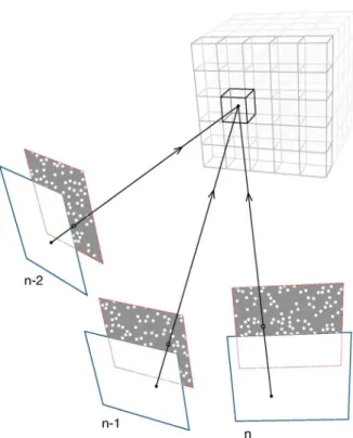
Fig. 2. Back projection: For a particular event, the accumulated totals at the target positions visible from the position of the event on the detector are in-creased. This includes the position of the actual source (dot in upper left region) — as well as some others.
One can think of this as accumulating “votes” for particular pixels or voxels. Alternatively, one can think of it as manipu-lating a quantity related to the probability that there is a source at a given location, or of estimating the strength of a radiation source at that location.
The basic algorithm can be described in pseudocode as: Reset accumulator array to zero;
For each detected event do { For each accumulator cell do {
if cell-to-detector ray intersects open mask cell do { increase total in accumulator cell;
} else do {
decrease total in accumulator cell; }
} }
Typically the main effort in the calculation is working out the geometry of the ray connecting the position of the event on the detector with the target cell, given the current geometric rela-tionship between the detector, the mask and the target volume. This part of the computation can be done efficiently using pre-computed lookup tables.
The “vote” added to an accumulator cell is not restricted to being a fixed amount — more generally, a “weight” can be added that may depend on geometric factors, such as, for ex-ample, exactly where the ray passes through the mask (whether it passes close to the edge of a hole or not). The weight can also be made to depend on the distance of the target cell from the point on the detector where the event was detected, as well as the direction of the ray. The choice of weighting function de-pends on the desired overall system point spread function (PSF)
Fig. 3. Radiation from a point in the target volume reaches the detector through open areas of the mask at three different times. The position and orientation of the detector system relative to the target volume is different in each of the three cases.
and considerations of noise and artifact suppression. There are the usual tradeoffs between resolution and noise [19].
Shown in Fig. 3 are positions and orientations of a detector system at three different times. Particular rays are shown passing through holes in the mask leading to points on the detectors where events are reported at those times.
Information about the position of each of these events on the detector, along with the known position and orientation of the detector and the mask relative to the target volume are used in back projection as shown in Fig. 4. In practice, of course, there would be thousands of events, not just three, but the same prin-ciple holds.
A. Overall Point Spread Function
The reconstructed image has spatial resolution limited by the size of detector elements, size of the mask holes, geometry of the apparatus and properties of the back projection algorithm. The “resolution” can best be described by a point spread func-tion (PSF). Typically, the term point spread funcfunc-tion is used to describe the spatial resolution of a linear shift-invariant system. The term as used here is a natural extension to a general linear system that is in fact not shift-invariant. The PSF may be deter-mined analytically, numerically or experimentally.
The PSF of the system including weighted back projection is typically anisotropic and spatially varying, becoming broader with distance from the detector system trajectory, and may have a characteristic “bow tie” shape. Deconvolutional “filtering” [20]–[22] tuned to the known PSF may be used after back projection to further improve the resolution. This is analogous
Fig. 4. Back projection of the three events through open areas of the mask, using the appropriate position and orientation for the detector system, adds to the accumulated total at the correct position in the target array. Accumulated totals at positions not “visible” from the event on the detector may be reduced.
to the post backprojection filtering described above in the discussion of tomography.
Since the PSF may be spatially varying, more sophisticated techniques than ordinary deconvolution may be required. Some improvement in the PSF or other properties of the reconstruc-tion may also be attained by “filtering” before the detector data is back projected. As in tomographic reconstruction, a judicious combination of pre- and postprojection filtering may be benefi-cial [17], [18].
With a spatially varying PSF, a question arises as to the proper scaling of reconstructed responses. There are two ob-vious choices: (i) make the peak response to a point source independent of position; or (ii) make the response to a uniform area source independent of position. In systems with constant PSF, the two criteria lead to the same result. The two schemes lead to different results, however, when the width of the PSF varies with position, since the latter makes the local integral of the response to point sources independent of position, rather than the peak of the response. The first approach tends to be more useful for imaging isolated point sources, while the latter makes more sense for extended sources.
B. Comparison With Existing Methods
Dynamic reconstruction is useful for imaging where a masked detector system is in relative motion with respect to a target area.
Traditional coded aperture systems, used in “staring” mode, require the geometric relationship between target, mask and de-tector to remain fixed. Relative motion between dede-tector system
and target may be unavoidable in some situations, or may ac-tually be introduced purposefully to extend the range or sensi-tivity of a detection system, or to provide the ability to image in three dimensions using only a two-dimensional detector system — or in two dimensions using only a one-dimensional detector system, as we demonstrate in the experimental section.
Sensitivity may be further enhanced due to the fact that infor-mation about objects in the environment is collected over some time while the detector system moves. If, for example, the de-tector moves in a line (perhaps mounted on a vehicle), then it collects information from a distant point over a time period that is directly proportional to the cross-track distance to that point. Normally, of course, the signal from a source falls off as one over distance squared, but since that source is now being ob-served over a time proportional to that distance, the accumulated detector signal used by the dynamic reconstruction method falls off only as one over distance, not distance squared. This reduc-tion in the exponent of signal drop off with distance from two to one is similar to that observed in synthetic aperture radar, and provides a powerful advantage when imaging remote, relatively weak sources [23], [24].
III. ADDITIONALREFINEMENTS ANDNOTES
There are different ways of organizing the dynamic recon-struction computation. It is possible, for example, to back project every event individually by stepping through each cell of the mask and projecting out onto the target accumulator array. Alternatively one can step through each pixel or voxel in the target accumulator array and determine whether the place where the event occured is visible through the mask from that location in the target area or volume — as shown in the pseudocode example above.
A precomputed mask array can be used to speed up the com-putation when stepping through the target array. The mask array need not be binary, but instead can have “weights” varying over some range. These may be based on how much of a detector cell is visible through a particular mask element. As an illustra-tion, an initially binary mask array may be convolved with the (suitably demagnified) detector PSF in order to take into account that each detector element responds over a finite area rather than being an infinitesimal point sensor. This accounts for the fact that a bundle of rays from a source area to a detector area passes through the mask rather than just a single ray.
A. Use of Nonideal Masks
In practice, nonideal mask/detector configurations may be de-sirable in order to limit cost, weight or size. Traditional coded aperture systems require four copies of a basic pattern that has the ideal bilevel autocorrelation property (or, less commonly, a single copy of the pattern and a detector array four times as large as the shadow of the mask). This may be prohibitively expensive or awkward to implement. Further, as the distance to the area of interest varies, so does the magnification of the mask shadow. This means that the part of the mask shadow sampled by the detector array is typically not one repetition of the basic mask pattern. Hence there has been interest in imaging with systems that do not have the ideal geometry for mask and detector or use
masks that do not have the ideal bilevel autocorrelation prop-erty.
In the case of an ideal mask and detector configuration, each point in the target illuminates the same total detector area through the mask, and in back projection, each target accumu-lator array element receives the same total contributions from detector elements. In the case of a nonideal mask configuration, however, different parts of the target may be “seen” by different numbers of detector elements through different number of holes in the mask. This causes reconstruction artifacts, manifesting themselves as “streaky” or “plaid” background textures. Such systematic artifacts can easily overwhelm the weak contrast between the signal at a target location and the large background pedestal accumulated in areas around it.
A normalization can remove, or at least suppress these arti-facts. Essentially, the idea is to back project a simulated, uniform detector frame to produce a reference target image, which is then used to correct future reconstructions. The reference image may be created, for example, by back projecting a detector frame in which every element has the same “count” or integrated flux. Later, back projected images from real data can be “normalized” by, for example, dividing by the stored reference image. Conve-niently, the reference image can be precomputed and stored for use after back projection of actual detector data.
B. Contrast-To-Noise Ratio (CNR)
A useful quantity in evaluation of the quality of reconstructed images is the CNR [15], which is the difference of the peak re-sponse to a “source” and the “background” or “pedestal” around the image of the source, divided by the standard deviation of the “background” or “pedestal.” One advantage of this quality mea-sure is that it is insensitive to manipulations of the reconstruc-tion process that merely scale all values or subtract an offset. The CNR depends on the image content (e.g., how much of the image area is occupied by “sources”), the parameters of the imaging system, as well as details of the reconstruction algo-rithm [15], [25]. The CNR is very high for a single point source, dropping as more sources are added. Generally the CNR is low when there are many sources, extended sources, or bright “back-ground” regions.
One use of experimentally estimated CNR values is in detector system calibration. Some parameters of the detector system — such as the distance and angular orientation of the mask relative to the detector array — may be hard to measure directly, but can be obtained by maximizing the CNR of images of a reference target such as a point source.
C. Computational Cost
The computational cost of the back-projection method is the order of additions or subtractions per event, where is the number of pixels or voxels in the resulting image — and hence the number of elements in the accumulator array. If there are a total of events, then the overall computational cost is . The inner loop computation depends on finding the intersection of rays with the mask, which can be done efficiently using lookup tables.
If events are “batched” by taking short exposure detector “frames” instead of back-projecting each event separately, then
the computation cost is multiplications and addi-tions, where is the average number of active detector ele-ments in a frame — which for high flux will be equal to , the number of detector elements.
For comparison, the computational cost of the traditional cor-relation decoding method, used with a stationary detector and mask, is multiplications and additions, where is the number of elements in the basic repeat pattern of the mask, since each of the pixel in the resulting image requires a cor-relation touching each of the pixels in the shadow of the mask. This is for the particular magnification where the mask shadow has exactly one repetition of the basic pattern on the de-tector array. As noted elsewhere, typically is about . D. Recovering Depth Information
A static coded aperture system can obtain some three-dimen-sional information by using the fact that the magnification of the mask shadow on the detector depends on the distance [15]. But the result is somewhat analogous to a “through focus stack” in optical microscopy, where points currently not in focus are still imaged, just smeared out. So what is seen in any one layer is the sum of what is in that layer and blurred versions of what is in other layers.
A moving detector platform, on the other hand, “views” a target from different directions which potentially enables proper recovery of three-dimensional information (just as CT can properly recover three-dimensional information, while laminography can not).
E. Resolution and Number of Pixels
The number of pixels or voxels used for reconstruction in the target accumulator is not limited by the sizes of mask ele-ments, detector elements or the overall geometry of the imaging system. However, it is not really useful to use pixels or voxels that are much smaller than the size of the PSF. A small amount of oversampling can be beneficial in that it avoids aliasing, but beyond a certain point one obtains only “empty magnification.” In static coded aperture imaging, the number of independent measurements possible is equal to the number of elements in the basic repeat pattern of the mask. This is also the number of independent pixel or voxels that can be recovered, since only that many different offsets can be used in correlation without repetition.
F. Dealing With the Finite Size of the Mask
There is an issue in back projection of what to do with rays that connect target elements to detector elements that miss the actual mask. This is a particularly important issue with non-ideal masks, with masks where the area around the mask is not shielded, and in the case of variable magnification of the mask shadow. It is possible to treat rays missing the mask as passing through completely closed or completely open areas of an ex-tended mask, depending on whether these areas are shielded or not. However, the resulting reconstructions have serious system-atic biases because the “pedestal” is no longer constant. Some-what suprisingly, it is better to pretend that the mask is in fact
an infinite doubly periodic pattern or to pretend that the area outside the actual mask has uniform transmission equal to the average transmission of the mask (i.e., equal to the fill factor). These heuristic methods tend to produce much less disturbing artifacts than methods that at first sight appear to more correctly model the physical reality.
G. Desirability of Masks With Low Fill Factors
The fill factor affects both the signal and the contrast. First, it should be pointed out that the term “fill factor” is variously used to refer to two different quantities: (i) the fraction of the mask area that is open; or (ii) the fraction of mask tiles that have an opening; Here mask tile is taken to be the elemental repeated shape that forms a tesselation of the plane. The two definitions give the same result if the opening in a mask tile is the whole tile. But when, for example, holes are drilled with centers on a square or hexagonal pattern, then such holes will not cover the full square or hexagonal mask tile and the first “fill factor” will be smaller than the second. Here it should be apparent from context which of the two meanings is intended.
In the original applications of coded aperture methods to X-ray astronomy, isolated point sources where typical and rela-tively high fill factors may have been appropriate. However, for nonpoint source targets and extended sources, lower fill factor masks, while giving up some signal, produce better CNRs [8], [9], [15], [19], [26].
The signal (peak minus pedestal) for each source location re-mains the same when more sources are added, while the back-ground (pedestal) grows linearly with the number of sources . The ratio of signal to background is correspondingly reduced as more sources are added.
A simlified analysis shows that the situation is improved when the fill factor is reduced since the signal is proportional to the fill factor while the pedestal is proportional to the square of the fill-factor. The contrast, i.e., peak minus pedestal, divided by pedestal, is
(1) for sources of equal strength. And, in this simple situation, the CNR is given by
(2) where is the strength of the sources, and the standard devia-tion of the noise in the pedestal is assumed propordevia-tional to the square root of the amplitude of the pedestal — as is appropriate for photon noise.
Many known ideal mask patterns have approximately 50% fill factor. Some ideal mask patterns are known that have approx-imately 25% fill factor. A mask with 25% fill factor has three times the contrast of a mask with 50% fill factor. The amplitude of artifacts tends to be lower with lower fill factors. A few pat-terns are known with smaller fill factors, but in general it is hard to find mask pattern designs with low fill factor that have the ideal bilevel autocorrelation property. This is one reason why being able to deal with nonideal patterns may be an advantage.
H. Nonplanar Masks and Nonplanar Detectors
Masks and detectors need not be constrained to lie in a plane. The method can be generalized to arbitrary arrangements of de-tectors in space and arbitrary arrangements of blocking (mask) elements. Since detectors block radiation, some or all of the de-tectors themselves can act as “mask elements” for radiation ap-proaching other detectors from certain directions. In this case there may be no need for separate “passive” blocking elements, or a separate “mask.” A simple example is a set of detectors disposed over the surface of a sphere with open areas between them. This can be used for simultaneously imaging in all direc-tions ( steradians) with detectors on one side of the sphere acting as “mask” for detectors on the other side of the sphere (see, e.g., the “coded sphere telescope” in [27]). Other arrange-ments may be envisaged of detectors and blocking elearrange-ments dis-posed in three-dimensional space.
IV. THEORETICALDERIVATION OFPOINTSPREADFUNCTION
Backprojection is a technique for reconstructing distributions from line (or plane) integrals. Examples are line integrals of emission (e.g., SPECT), line integrals of absorption (e.g., CT), and line integrals of nuclear resonance response (e.g., MRI). The value recorded by a detector for a particular line is “back projected” along that line (or plane). The accumulated total at a particular point is the integral over all lines passing through that point.
In the two-dimensional case, lines can be parameterized using the angle between the line and the axis, and the perpendic-ular distance from the origin to the line. The perpendicular distance of a point from the line is
(3) Thus the line is just the locus of points for which . Corre-spondingly
(4) is zero everywhere except on the line — and has unit integral along a perpendicular to the line. If the weighted signal for this line is , then the overall result of backprojection is the integral over all lines
(5) Now most lines do not pass through the point and thus will not contribute to the back-projected result at that point. We need only consider a subset of lines in the integral. Let us suppose that at time during a scan, the line is the one that passes through the point . Then we can rewrite the expression for
as
(6) (We could also use a parameter other than time here.)
It is often convenient to group the lines in such a way that lines passing through a common point are treated together. In the case of fan-beam CT, for example, such a point could be the
X-ray source. The fan of rays emitted from the X-ray source at a particular position in its circular trajectory around the object being scanned can be treated as a group. Similarly, in the case of pinhole imaging, the fan of rays passing through the pinhole at a particular position in its trajectory can be treated as a group. In each case, only one ray in the group passes through the point and needs to be considered.
The trajectory of the point common to the subsets of lines is of importance in determining the properties of the backprojected result. In the case of CT, this is the trajectory of the X-ray source, while in the case of a pinhole camera the trajectory of interest is that of the pinhole.
Backprojection does not produce the distribution of emitting or absorbing material directly. The output of backprojection is the result of a general linear operation on the desired underlying distribution. This linear operation can be thought of in terms of a (possibly spatially varying) point spread function (PSF) that depends on the trajectory. If it happens to be spatially invariant, then it is a convolution, in which case it can be compensated for using deconvolutional filtering of the back-projected result.
Weighting the detected signal before backprojection alters the PSF and can be used to make it more amenable to further pro-cessing. It may, for example, be used to make the PSF rotation-ally symmetric or even spatirotation-ally invariant. Finrotation-ally, projection data of subsets of lines may be filtered and weighted before back projection to affect the PSF. In favorable cases such prefiltering can be equivalent to postbackprojection deconvolution. A. Simplified Model
To study the features of the PSF of back projection algo-rithms, we’ll first consider a single pinhole and assume a single point source at the origin. Rays from the source through the pin-hole strike the detector array in a place that depends on the posi-tion and orientaposi-tion of the detector system as it moves along its trajectory. The detected value is then backprojected along the same ray and contributes to the accumulated totals — with the highest contribution at the position of the source.
The value back-projected is proportional to the flux at the de-tector system, which will depend on the inverse of the square of the distance from the source to the pinhole, but may also depend on foreshortening of areas because of the angle between the ray and the normal to the detector or mask surface. Further, we’ll see that it can be advantageous to weight the backprojected values according to the current position and orientation of the detector system in a fashion that depends on the chosen trajectory.
Of course, coded aperture masks have multiple holes, not just a single one. But in some commonly used configurations each hole contributes to the reconstruction of the point source in the same fashion. Thus in the case of a single point source, the PSF for the multihole case is simply a multiple of the result for a single hole.
Masks have holes of finite size, not pinholes. This introduces some “blurring.” In practice, the overall point spread function can be treated as the convolution of the point spread function for an ideal pinhole with a “blur” function corresponding to the shadow of a mask hole cast on the target from a point on the detector — or, cast by points distributed over all of a detector element.
Fig. 5. General trajectory with respect to point source.
Also, one is typically not dealing with a single point source, but many point sources, or extended sources. If the mask has the ideal bilevel autocorrelation property, the contributions at a point, from all but the radiation from that particular point, will produce a background “pedestal” that is spatially invariant and so can be subtracted without affecting the PSF. Overall, the simple model of a pinhole and a point source allows one to get at the core of the point-spread function issue.
B. Model of Projection and Back Projection
To study the dependence of the PSF on the trajectory and on the backprojection weighting scheme, consider the dynamic reconstruction of a point source at the origin of a coordinate system when the detector system moves along a trajectory in the - plane as shown in Fig. 5.
Suppose the point moves along a curve . A line connecting the origin to the point has length and makes an angle with the -axis. The perpendicular distance of a point from this line is given by
(7) Consequently the contribution made to the accumulated total at the point in back-projection at a particular time is proportional to
(8) Integrating over time we find the PSF
(9) where is the value used when backprojecting from the po-sition of the detector system .
We can change variables if varies monotonically (10)
where now expresses the value to be backprojected as a function of angle rather than time, while and
. Now
(11) if is the only value of for which . Here
(12) (13) Now , , with , so (14) and so finally (15) where is the PSF now expressed in polar coordinates. So the PSF is always proportional to , but may also have some dependence on . This dependence on can be removed, if de-sired, simply by weighting the backprojected values with . If, for example, the motion along the trajectory has a fixed ve-locity, then is proportional to the cosine of the angle be-tween the normal to the trajectory and the vector , and inversely proportional to the distance from the origin. C. Example: Circular Scan Tomography
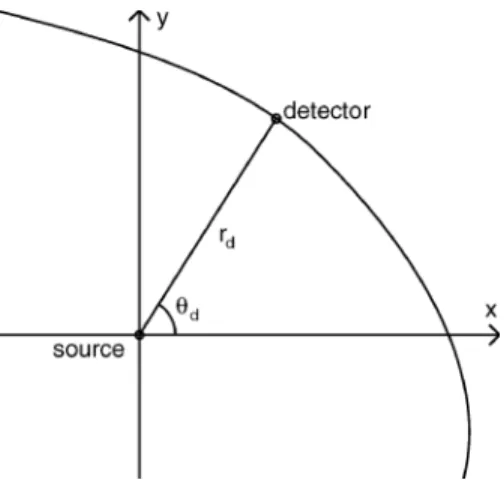
As a specific illustration, consider a tomographic system with a circular, constant angular velocity source trajectory and as-sume for now that there is an attenuating object at the origin as shown on the left in Fig. 6.
Here the detector signal is constant, say, as is the angular rate , so
(16) yielding the response of unfiltered backprojection.
Taking the Fourier transform produces the system response, which is proportional to , where is the magnitude of the spatial frequency. This “low frequency emphasis – high fre-quency deemphasis” can be compensated for after backprojec-tion by using a two-dimensional “ramp” filter whose response is proportional to the magnitude of the spatial frequency (up to some limiting frequency). For parallel beam projections it can equivalently be compensated for by using a one-dimensional “ramp” filter before back-projection on each collection of par-allel lines [16].
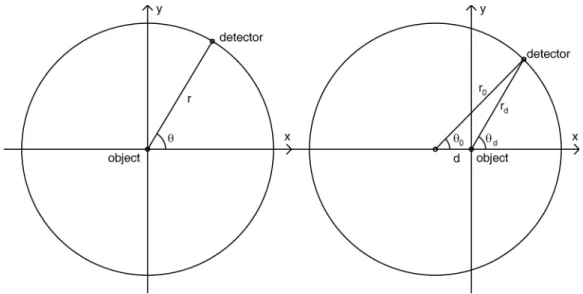
The situation is a bit more complicated if the attenuating ob-ject is off-center relative to the circular traob-jectory, as shown on the right in Fig. 6. In this case, the angular rate varies, so that, simple back-projection would produce an anistropic PSF. The departure from circular symmetry grows with the distance
Fig. 6. Circular trajectory with respect to attenuating object. On the left, the object is at the center of the circular trajectory. On the right, the object is off center.
of the attenuating object from the center of the trajectory. How-ever, the angular rate does change in a predictable fashion, so that we can simply weight the values to be backprojected by multiplying by , where
(17) and , so . We can multiply by
(18) to once again obtain a rotationally symmetric PSF. This cor-responds to the weighting required before back-projection in fan-beam reconstruction algorithms [18].
One can view parallel beam CT as fan beam CT in the limit as the radius of the trajectory tends to infinity. In this case, the variation in the point spread function with position can be ig-nored and the result of backprojection is simply the underlying density distribution convolved with a PSF proportional to . D. Example: Linear Scanning Trajectory
Now consider instead a detector system moving at constant velocity along a straight line with the detectors oriented to look out “across track.” Let the trajectory be parallel to the axis with the distance of closest approach of the detector system to the source at the origin as shown in Fig. 7. So and , where is the linear velocity along the track.
Here . So and
(19) (for ). We again see the dependence, but also an apparent increase in response as approaches . This is because the angular rate slows as the angle increases, al-lowing the accumulated totals to grow more for larger angles. However, the radiation flux per unit area from the source also drops, since it is proportional to the inverse square of the dis-tance of the detector from the source, where .
Thus the inverse square law reduction in flux actually cancels out the dependence of on and we obtain
(20) So, if we were to ignore other factors, we would obtain the same rotationally symmetric PSF as in the case of parallel beam to-mography discussed above.
Now, if the array of detectors lies along the track, oriented to respond maximally to a signal from across track, then there will be foreshortening of the apparent area exposed to radiation from the source unless . The apparent or foreshortened area is proportional to . Overall, then the measured signal actually drops off according to the well known “cosine cubed law” (see, e.g., [28, eq. 6, p. 247]). So we actually end up with
(21) To get an idea of what this PSF looks like, consider the contours of constant response, which, in polar coordinates, have the form for constant . That is , or ,
or . Hence
(22) These are circles of radius , with centers at — all tangent to the axis at the origin. This yields a “bow tie” shape, with “wings” oriented vertically (i.e., across track) as shown in Fig. 8.
We can, of course, elect to compensate for the depen-dence by weighting the signal from the detector before backpro-jection by multiplying by . This again leads to a circularly symmetric PSF proportional to , as above. There is some price to pay for this, since the weaker signals obtained when far from the source (i.e., for large ) would be amplified along with the noise in those signals. Thus the improvement in the PSF would be accompanied by some increase in the noise of recon-struction.
Fig. 7. Linear trajectory with detector system oriented to look “across track.”.
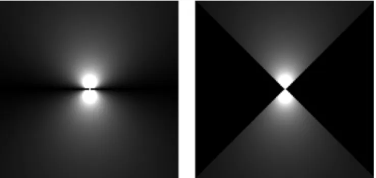
Fig. 8. Two representations of the PSF for the linear trajectory detector system. On the left, response proportional to density of lines (ignoring the Moiré inter-ference effects). On the right, contours of constant response.
Fig. 9. “Bow tie” PSF for unlimited detector system FOV on the left — and for limited FOV on the right.
Now in practice, the mask and detector arrangement has a finite field of view, determined by the ratio of the separation of the mask from the detector and the size of the detector or the mask. This means that the above integral is not over the full range to , but say from to . The result is that the point spread function is truncated, multiplied by where
for
otherwise (23)
The PSF shown on the left in Fig. 9 is for unlimited FOV, while that one on the right is for the case when the FOV is lim-ited to . The truncation makes the PSF look even more like a “bow tie” and corresponds to the limited-angle case in CT.
Fig. 10. One-dimensional mask pattern used in moving gamma ray detector array, based on quadratic residues forp = 19.
V. EXPERIMENTS
A. Moving Large Area Detector Simulation
A moving large area detector array was constructed by Ziock et al. for detecting radioactive material at a distance [23], [24]. It uses a one-dimensional detector array with a coded aperture mask based on two repetitions of the quadratic residue pattern for (Fig. 10). Each of the 19 vertical detector strips is made up of a stack of three 100 mm 100 mm 100 mm NaI scintillators coupled to photomultipliers. The coded aper-ture mask is 1 m from the detector array and made of 40 mm thick Linotype metal slats with 108 mm pitch designed to match the spacing of the detector elements.
Simulation data were generated using the known geometry of the mask and detector array, with small radiation sources across track. The detector system was assumed to move in a straight line at a constant velocity of 8.94 m/s (20 mph) in a direction parallel to the long axis of the detector array. Three sources off to the side of the array (“cross track”) were simulated. In order of appearance: 74 MBq (2 mCi) at 100 m, 18 MBq (0.5 mCi) at 25 m, and 37 MBq (1 mCi) at 50 m. The background rate was 500 counts per second per square meter.
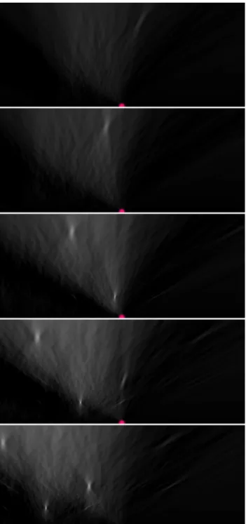
Dynamic reconstruction was performed in a vehicle-centric coordinate system. In Fig. 11, the large area imaging detector array is located where the bright dot is in the middle of the bottom edge of each of the rectangular images. The image areas shown in each case is 120 m 570 m. The image is “developed” as the vehicle moves from left to right. The image is slid off to the left at the same rate as the vehicle moves, so that the detector system is stationary in the image coordinate system. The three sources are detected in turn as the detector system passes them. For this sequence, the overall number of events detected was about 18 000 — including about 10 000 background events.
In addition to spots at the appropriate source locations, some streaky artifacts are also visible. These occur mostly at angles that correspond to places where a source first enters the field of view and where it exits the field of view of the mask and detector system. The anisotropic nature of the PSF is visible, with characteistic “bow-tie” shape.
The increase in size of the PSF with distance is also apparent. Generalized deconvolution (for the spatially varying case) could be used to make the PSF closer to ideal (impulse like). However, for purposes of detecting sources of radioactivity, this form of presentation is adequate (it is clear that there are three sources,
Fig. 11. Frames 80, 120, 160, and 200 of a sequence produced by dynamic reconstruction of simulated data for a moving large area imaging array. The bright dot in the middle of the lower edge indicates the position of the detector system.
that they are at distances of 25, 50, and 100 m, and so on). Also, deconvolution would increase noise and accentuate arti-facts. Note that each “blob” corresponding to a particular source develops as the vehicle moves past the source, being noticeable when the source is across track, but being fully formed only sometime after the vehicle has passed.
B. Gamma Camera and Coded Aperture Mask
An ISOCAM gamma camera from Park Medical System, was equipped with a coded aperture as shown in Fig. 12. The gamma
Fig. 12. Moving coded aperture imaging system using gamma camera and hexagonal mask array.
camera uses 86 photomultipliers to determine the location of an event in a 12.7 mm thick NaI crystal scintillator plate with an effective sensitive area of 420 mm 536 mm and 2.7 mm FWHM resolution (5.1 mm FWTM). Positional readout is quan-tized to multiples of 0.672 mm. A hexagonal mask with 3.1 mm diameter holes spaced 3.5 mm apart based on quadratic residues (50% fill factor) for [13] was drilled in a 3.2 mm thick 600 mm 600 mm lead alloy sheet. The mask was mounted on a lead-shielded box with a truncated-pyramid shape at a distance of 682 mm from the gamma camera. Readout of the gamma camera during relative motion between the de-tector system and the target was used to provide input for the dynamic reconstruction algorithm.
The exact distance of the mask and the angular orientation of the mask relative to the gamma camera was determined using small sources of and . Reconstructed images of very high contrast and resolution of these small sources are obtained when the correct parameters are used in reconstruction. C. Area Source
In the first experiment, the target was a uniform isotopic area source (Featherlite rectangular flood source 185 MBq (5 mCi) 640 mm 455 mm), parts of which where occluded by lead cutouts placed in front of it as shown on the left in Fig. 13. The energy window in the gamma camera was set to 110–134 keV. One frame of the dynamic reconstruction sequence is shown on the right in Fig. 13. The CNR is not very good. As discussed above, 50% fill factor mask patterns commonly used for imaging point sources are not ideal for imaging area sources or extended sources.
D. Lower Fill Factor — Biquadratic Residue Pattern
Consequently a second mask, with 3.5 mm diameter holes spaced 3.9 mm apart, based on biquadratic residues (25% fill factor) for [13] was drilled.
Shown in Fig. 14 are two frames out of a sequence of re-constructions made as the distance between the detector system and the target was steadily reduced. The second reconstruction
Fig. 13. Isotopic area source partially occluded by some lead bricks and lead plate cutouts, and one frame of dynamic reconstruction sequence using 50% fill factor mask.
Fig. 14. Two frames from a dynamic reconstruction sequence of an isotopic area source partially occluded by some lead cutouts using the 25% fill factor mask.
has better CNR because more information has been accumu-lated about the target. (Only one depth plane of reconstruction is shown.)
Note the small vertically oriented rectangular response in the right-hand reconstructed image below the left edge of the cir-cular region. This corresponds to a small gap between the lead plate cutours that is not visible in the left-hand reconstruction. E. Backscattered X-Rays
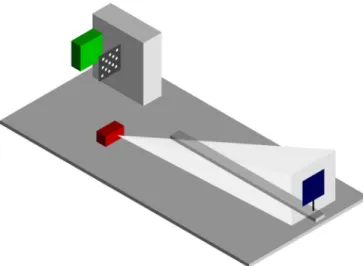
The detector system described above can also be used to image back-scattered X-rays. A 225 keV, 13.5 mA X-ray source provided by American Science and Engineering (ASE), positioned on the floor to the right of the detector system was used to illuminate an area of about 0.75 m diameter about 5 m from the detector system, as shown in Fig. 15. The actual area illuminated by X-rays is outlined by small pieces of tape stuck on the wall as seen in Fig. 16.
Targets were then introduced between the detector system and the wall. The targets where mounted on a carriage that could be moved between 5 m from the detector system to 2 m during data acquisition. The mean backscatter energy was measured to be 113 keV, so the energy window in the gamma camera was set to 104–125 keV.
Acquired gamma camera output data were then used as input to the dynamic reconstruction algorithm. The trajectory in this experiment is more or less along the line connecting the target to the detector, unlike the large area imaging system described earlier where the target area lay “across track.” This means that the PSF here is elongated in the direction along track (“depth”)
Fig. 15. Geometry of backscatter X-ray system used in dynamic reconstruction experiments. The box at the top is the gamma camera equipped with a mask. X-rays from the source on the floor near the camera illuminate a target mounted on a carriage that can be driven to vary the distance between the gamma camera and the target during data acquisition.
Fig. 16. Polyethelene arrow and polyethelene annulus used in X-ray backscatter experiment. Tape strips outline the area on the wall illuminated by X-rays.
and so the above noted anisotropy of the PSF is not apparent in slices taken more or less perpendicular to the track.
1) Polyethylene Arrow: One target was an upward pointing arrow cut out of a thick polyethelene sheet as shown on the left in Fig. 16 (arrowhead width 355 mm, shaft width 155 mm, overall height 584 mm, and thickness 102 mm). Plastic was chosen as the material because of the low atomic number of its con-stituents (hydrogen 1, carbon 6). Materials containing atoms of low atomic number scatter X-rays back more strongly than those of high atomic number. This makes organic materials, plastics and many explosives appear brighter in this mode of imaging than, for example, most metals.
Dynamic reconstruction recovered the arrow but also shows significant backscatter from the wall behind the target as shown in Fig. 17. This is not surprising, since concrete contains var-ious oxides and hydrates which contain atoms of low atomic number (hydrogen 1, oxygen 8). In an attempt to reduce this ef-fect, a steel plate was added in front of the concrete, but even steel produces quite a bit of backscatter. This limits the contrast attainable in this particular experimental configuration — and also dictates use of low fill-factor masks.
2) Polyethylene Annulus: Another target imaged with the 25% fill factor mask was the polyethelene annulus shown on the
Fig. 17. Two frames from a dynamic reconstruction sequence of X-ray backscatter from a polyethelene arrow using the 25% fill factor mask. Note also the backscatter from the wall behind the target.
Fig. 18. Two frames from a dynamic reconstruction sequence of X-ray backscatter from a polyethelene annulus using the 25% fill factor mask. Note the shadow cast on the wall behind the target.
right in Fig. 16 (outer diameter 350 mm, inner diameter 80 mm, and thickness 102 mm). Again, two frames from a sequence pro-duced by dynamic reconstruction are shown in Fig. 18. The one on the right has considerably better CNR than the one on the left because more information about the target had been collected at that point ( versus detected photons overall).
3) Water Bottle: Water, of course, is also a good backscat-terer of X-rays. A five gallon water bottle shown in Fig. 19 (di-ameter 305 mm and overall height 560 mm) was used for an-other experiment. A frame from a dynamic reconstruction se-quence is shown in Fig. 19. In the reconstruction note the some-what darker area on the right corresponding to the cutout for the carrying handle. There is also a narrow X-ray shadow cast on the background to the left and above the bright area of the image of the water bottle itself. A shadow is cast there because the source of X-rays is to the right and below the detector system. It is no-ticeable in the image because the background material also scat-ters back a significant number of X-rays and is “lit up” except where it is shadowed by the target. The neck of the bottle does not show up bright in the reconstruction because the water level did not reach up into the neck.
F. Lower Fill Factor — Octic Residue Pattern
Since low fill factors are more suited to imaging extended sources, a third hexagonal mask with 1.45 mm holes spaced 1.625 mm apart based on octic residues (12.5% fill factor) for
[13] was drilled in 3.2 mm thick lead alloy. The overall image quality and the CNR obtained with this configuration was lower than for the 25% fill factior mask. The
Fig. 19. Five gallon water bottle used in X-ray backscatter experiment and a frame from the dynamic reconstruction sequence using the 25% fill factor mask.
reason for the low quality is that the hole size (1.45 mm) and spacing (1.625 mm) of this mask are below the resolution (2.7 mm FWHM) of the gamma camera.
The reason this fine mask can be used for imaging at all is that the mask pattern does contain lower spatial frequencies as well, which can be imaged by the gamma camera. However, the available spectral energy in the mask is spread over a wider frequency spectrum so that less is available in the low frequency area accessible for imaging by this particular gamma camera. The small hole size and spacing was forced by the choice of an octic residue pattern. There are very few octic residue patterns having the ideal bilevel autocorrelation property (
) [13].
VI. APPLICATIONS
Some applications of dynamic reconstruction arise naturally where coded apertures or tomography are presently used. Ad-ditional applications are enabled by the possibility of imaging while there is relative motion between target and detector system. The following are some examples:
A large area can be searched for radioactive material, such as “Special Nuclear Materials” (SNM) or “Radiological Disper-sive Devices” (RDD) using a mobile system that accumulates information as the detector system moves through an area [23], [24]. While such systems have been built, reconstruction has been based on traditional coded aperture methods, such as cor-relation, applied to data collected over intervals of time short enough that motion was relatively small. The results of these individual “quasi static” reconstruction were then aligned and added together to lead to a “quasi dynamic” reconstruction.
Another application is that of search for objects composed mostly of low atomic number materials (such as explosives or drugs) using back-scattered X-rays. Backscattered X-rays are already being used in search for contraband, but some such sys-tems depend on using a pencil beam along with large area de-tectors that have no spatial resolution. Such systems tend to be inefficient in their use of radiation since the pencil beams are generated by discarding almost all of the radiation from a tradi-tional X-ray source.
A system using dynamic reconstruction can instead “flood-illuminate” an area of interest and image the returned radiation using a moving coded aperture system. This has the potential of increasing the speed of image acquisition and the image quality — although coded aperture imaging systems do lose the fraction of the backscattered radiation that does not make it through the mask — a particular concern with masks of low fill factor.
VII. SUMMARY ANDCONCLUSION
Dynamic reconstruction enables use of moving masked de-tector systems when imaging with radiation that cannot be re-fracted or reflected. The method can be viewed as geometri-cally guided, weighted back projection and provides the poten-tial for recovering depth. In some configurations, the sensitivity drops off as the inverse of distance from the target rather than the square of the inverse of the distance. The point spread func-tion can be tuned by weighting the backprojected contribufunc-tions based on ray directions and distances. Dynamic reconstruction can be used with coded aperture masks and gamma cameras, or with other combinations of absorbers and detectors and with various trajectories for the detection system relative to the area or volume being imaged.
ACKNOWLEDGMENT
American Science and Engineering kindly provided a 225–keV 13.5–mA X-ray source for the experiments.
REFERENCES
[1] E. E. Fenimore and T. M. Cannon, “Coded aperture imaging with uni-formly redundant arrays,” Appl. Opt., vol. 17, no. 3, pp. 337–347, Feb. 1978.
[2] W. R. Cook, M. Finger, T. A. Prince, and E. C. Stone, “Gamma-ray imaging with a rotating hexagonal uniformly redundant array,” IEEE
Trans. Nucl. Sci., vol. 31, pp. 771–775, Feb. 1984.
[3] M. H. Finger and T. Prince, F. C. Jones, Ed., “Hexagonal uniformly redundant arrays for coded-aperture imaging,” in Proc. NASA
God-dard Space Flight Center 19th Int. Cosmic Ray Conf., 1985, vol. 3,
pp. 295–298.
[4] S. R. Gottesman and E. E. Fenimore, “New family of binary arrays for coded aperture imaging,” Appl. Opt., vol. 28, no. 20, pp. 4344–4352, Oct. 1989.
[5] J. J. M. in ’t Zand, Coded Aperture Imaging in High-Energy As-tronomy 1996 [Online]. Available: http://astrophysics.gsfc.nasa.gov/ cai/coded_intr.html
[6] I. D. Jupp, A. R. Green, and A. J. Dean, Optimised Sampling for
Hexag-onal Array Coded Mask Telescopes. Boston, MA: Kluwer Academic, 1995, p. 203.
[7] A. Busboom and H. D. Lueke, “Hexagonal binary arrays with perfect correlation,” Appl. Opt., vol. 40, no. 23, pp. 3894–3900, 2001. [8] E. E. Fenimore, “Coded aperture imaging — predicted performance
of uniformly redundant arrays (T),” Appl. Opt., vol. 17, no. 22, pp. 3562–3570, Nov. 1978.
[9] E. E. Fenimore, “Coded aperture imaging — the modulation transfer function for uniformly redundant arrays,” Appl. Opt., vol. 19, no. 14, p. 2465, 1980.
[10] D. Calabro and J. K. Wolf, “On the synthesis of two-dimensional array with desirable correlation properties,” IEEE Inf. Control, vol. 11, p. 530, 1968.
[11] C. Brown, “Multiplex imaging with multiple-pinhole cameras,” J.
Appl. Phys., vol. 45, no. 4, pp. 1806–1811, Apr. 1974.
[12] S. W. Golomb and G. Gong, Signal Design for Good Correlation. Cambridge , U.K.: Cambridge Univ. Press, 2005.
[13] B. K. P. Horn, “Sequence with bilevel auto-correlation property equals its own DFT,” IEEE Trans. Image Process., 2010, submitted for publi-cation.
[14] E. Caroli, J. B. Stephen, G. di Cocco, L. Natalucci, and A. Spizzichino, “Coded aperture imaging in X- and gamma-ray astronomy,” Space Sci.
Rev., vol. 45, no. 3-4, pp. 349–403, Jan. 1987.
[15] R. Accorsi, “Design of near-field coded aperture cameras for high-res-olution medical and industrial gamma-ray imaging,” Ph.D., MIT, Cam-bridge, 2001.
[16] A. C. Kak and M. Slaney, Principles of Computerized Tomographic
Imagaing. New York: IEEE , 1988.
[17] B. K. P. Horn, “Density reconstruction using arbitrary ray sampling schemes,” Proc. IEEE, vol. 66, pp. 551–562, May 1978.
[18] B. K. P. Horn, “Fan-beam reconstruction methods,” Proc. IEEE, vol. 67, pp. 1616–1623, Dec. 1979.
[19] G. K. Skinner, “Sensitivity of coded mask telescopes,” Appl. Opt., vol. 47, no. 15, p. 2739, May 2008.
[20] W. H. Richardson, “Bayesian-based iterative method of image restora-tion,” J. Opt. Soc. Amer., vol. 62, no. 1, pp. 55–59, 1972.
[21] L. B. Lucy, “An iterative technique for the rectification of observed distributions,” Astronom. J., vol. 79, no. 6, pp. 745–754, 1974. [22] P. C. Hansen, J. G. Nagy, and D. P. O’Leary, Deblurring Images —
Matrices, Spectra and Filtering. Philadelphia, PA: SIAM, 2006. [23] K. P. Ziock, W. W. Craig, L. Fabris, R. C. Lanza, S. Gallagher, B. K. P.
Horn, and N. W. Madden, “Large area imaging detector for long-range, passive detection of fissile material,” IEEE Trans. Nucl. Sci., vol. 51, pp. 2238–2244, Oct. 2004.
[24] K. P. Ziock, J. W. Collins, W. W. Craig, L. Fabris, R. C. Lanza, S. Gal-lagher, B. K. P. Horn, N. W. Madden, E. Smith, and M. L. Woodring, “Source-search sensitivity of a large-area, coded-aperture, gamma-ray imager,” IEEE Trans. Nucl. Sci., vol. 53, pp. 1614–1621, Jun. 2006. [25] R. Accorsi, F. Gasparini, and R. C. Lanza, “Optimal coded aperture
pat-terns for improved SNR in nuclear medicine imaging,” Nucl. Instrum.
Methods in Phys. Res. A, vol. 474, no. 3, pp. 273–284, Dec. 2001.
[26] J. J. M. in ’t Zand, J. Heise, and R. Jaeger, “The optimum open fraction of coded apertures with an application to the wide-field X-ray camera of SAX,” Astron. Astrophys., vol. 288, pp. 665–674, 1994.
[27] A. J. Bird and M. R. Merrifield, “X-ray all-sky monitoring and transient detection using a coded sphere telescope,” Astron. Astrophys. Suppl.
Ser., vol. 17, pp. 131–136, May 1996.
[28] C. G. E. Orton, Radiation Dosimetry: Physical and Biological