HAL Id: hal-00296766
https://hal.archives-ouvertes.fr/hal-00296766
Submitted on 23 Jun 2003
HAL is a multi-disciplinary open access
archive for the deposit and dissemination of
sci-entific research documents, whether they are
pub-lished or not. The documents may come from
teaching and research institutions in France or
abroad, or from public or private research centers.
L’archive ouverte pluridisciplinaire HAL, est
destinée au dépôt et à la diffusion de documents
scientifiques de niveau recherche, publiés ou non,
émanant des établissements d’enseignement et de
recherche français ou étrangers, des laboratoires
publics ou privés.
Noise variance estimation and optimal weight
determination for GOCE gravity recovery
J. Kusche
To cite this version:
J. Kusche. Noise variance estimation and optimal weight determination for GOCE gravity recovery.
Advances in Geosciences, European Geosciences Union, 2003, 1, pp.81-85. �hal-00296766�
c
European Geosciences Union 2003
Advances in
Geosciences
Noise variance estimation and optimal weight determination for
GOCE gravity recovery
J. Kusche
Department of Geodesy, Delft University of Technology, Thijsseweg 11, 2629, JA Delft, The Netherlands
Abstract. In the course of level 2 data processing for the
GOCE (Gravity Field and Steady–State Ocean Circulation Explorer) satellite mission different streams of level 1b data will be merged in a single solution providing the Earth’s gravity field, but also state-vector parameters and other quan-tities. A proper weighting of orbit tracking data, gravity gra-diometry data and certain a priori information, usually con-sidered as ‘solution constraints’, can be expected as crucial for the solution quality. But the a priori stochastic models, based on pre–mission assessment of the expected instrument behaviour, may be over–optimistic or even too pessimistic since they refer to an unprecedented mission with scientific payload never tested in space. One way to derive an opti-mal weighting scheme on a statistically sound basis while simultaneously validating the stochastic noise levels of the data is by including variance component estimation as a part of the level 1b to level 2 data analysis process. The idea is that by applying Monte-Carlo techniques this method can be extended to a large-scale problem like GOCE data analysis, using software modules that already exist or are currently under development. The proposed method has been tested using simulated GOCE orbit trajectories as well as gravity gradiometry data corrupted by colored random noise.
Key words. GOCE, gravity field modelling, combination
solutions, weight estimation, variance component estimation
1 Introduction
As its main product, ESA’s Gravity and Steady-State Ocean Circulation Explorer Mission (GOCE) will provide a global model of the Earth’s static gravity field (ESA 99). The com-putation of this model will rely on different level 1b data sets that should be processed ideally in a joint parameter esti-mation scheme. This includes at least satellite gravity gra-diometry data derived from different accelerometer combi-nations, and satellite-to-satellite tracking data from the GPS
Correspondence to: J. Kusche ([email protected])
system. Depending on the solution strategy and objectives, airborne data collected over the Earth’s polar areas, gravity data or models provided by the current missions CHAMP or GRACE, or adopted a priori constraints on high-degree sig-nal power may be used in the asig-nalysis.
Needless to say that the choice of the relative weights for these data sets or models is of vital importance for obtaining the most reliable estimates of the spherical harmonic coef-ficients, the level 2 product. But also the reliability of the estimated covariance matrix of the gravity field solution will depend on the assumptions about the observation weights. We propose therefore, that a weight optimization process on a stochastic basis should be included in the level 1b to level 2 (hereafter abbreviated as L2) data processing. Although a lot of effort is currently put into the pre-mission investiga-tion of error models for the gradiometer instrument and the precise orbit determination (POD) process, and into in-flight calibration and error assessment strategies that apply before arriving at the level 1b (Koop et al., 2002), optimization with respect to the weights given by these models within the L2 processing may still improve the final product. At the same time it would serve as a validation of the a priori stochastic models, when real data becomes available. However, also the functional models implemented in the processing will suffer from imperfections, e.g. an aliasing effect might occur due to truncation of the spherical harmonic expansion, and the sen-sor models will simplify the measurement process. On the one hand, adjusting the stochastic models in a joint estima-tion process will to a certain extend compensate for this func-tional mismodelling, on the other hand these effects must be taken into account when interpretating the estimated stochas-tic parameters.
The method investigated in this paper relies on a statisti-cal basis, i.e. the (almost) unbiased estimation of variance components (VCE), see e.g. Grafarend et al. (1980) or Koch (1990). Looking at the present GOCE data analysis concepts, the main limitation of VCE techniques so far seems the costly and repeated computation of the redundancy contributions of the observation groups, which equal to the trace of the
so-82 J. Kusche: Noise variance estimation called observation group influence matrices. The latter is
the projection matrix which relates a particular observation group to the corresponding least-squares adjustment residu-als; it involves the normal matrix contribution of the particu-lar data set as well as the inverse of the weighted combined normal matrix. For large systems, like those encountered when solving for a high-resolution gravity field model within GOCE L2 processing, this appears prohibitive. Therefore we propose a variant described by Koch and Kusche (2002), which makes use of a stochastic trace estimation technique invented by Girard (1989) and Hutchinson (1990). It has been recently (Kusche, 2003) re-structured and developed further in a Monte-Carlo sense (and called MCVCE), that is, on input for an arbitrary least-square inversion software we use cyclically randomized versions of the original data set where for each observation group in question an artificial noise sequence has to be passed through the inversion. On output, from a comparison of the residuals obtained with the original data and the randomized data the variances are esti-mated and new weights are chosen in an iterative sense. The main advantage is, that basically an existing software pack-age for solving the L2 inversion problem can be used without modifications.
The material is organized as follows: First, we briefly re-view the particular iterative VCE algorithm we intend to use. We will explain how this algorithm can be ‘mimicked’ by embedding a given L2 inversion program in a Monte Carlo framework, that is, by passing artificially generated random data through the inversion. Finally, two simulations un-der rather simplified condition show how a priori stochas-tic models for GOCE data can be validated and improved by MCVCE: We consider (1) low-degree gravity field recov-ery from the GPS orbit determination, where the noise level varies between different (1 day–) orbital arcs, and 2) a si-multaneous assessment of the total gradiometer noise power (variance) and the total power of an a priori signal degree variance model. A discussion closes this contribution.
2 Methodology
The linear observation model, which shall be adopted here for the joint inversion of p independant observation groups collected from GOCE, reads
Xiβ = yi+ei i ∈ {1, . . . , p} . (1)
The ni ×umatrices Xi are the design matrices, the u × 1
vector β represents the unknown spherical harmonic coeffi-cients plus additional unknowns such as state–vector param-eters, the ni×1 vectors yi contain the observations, and the ni ×1 vectors ei the stochastic observation errors. The
ob-servation vectors may be internally correlated (the noise may be coloured) but are assumed to be uncorrelated with respect to each other. Moreover, we assume that the covariance ma-trices of these observation groups are known a priori only up
to some scaling factors, the p noise levels or variance com-ponents σi2:
E(eie0j) =0 E(eie0i) = σi2P −1
i . (2)
This means, that the total number of unknowns in our prob-lem is u + p. The actual number p of these subdivisions of the overall GOCE data set, corresponding to the number of degrees of freedom in the stochastic model, will be a part of the solution strategy and as such subject to individual consid-erations and growing experience in the course of the L2 pro-cessing phase. If only the weighting between GPS-derived precise orbit (POD) data and gradiometry data as a whole is considered, p equals to 2. If, in addition, we allow for adjust-ing the weight of a priori information (contrainadjust-ing the very high degrees), p equals to 3. If one breaks off the stochas-tic model by allowing for varying noise levels in time, e.g. after orbit manoeuvres, internal re–calibrations, or between orbital arcs, and in space, e.g. between the different gra-diometer components, p might become reasonably large.
The estimation of variance components σi2(Grafarend et al., 1980; Koch 1990) leads generally to a coupled iterative process, since both the calculation of the so–called group re-dundancies ri (see below, step 4) as well as of the residuals ˆ
ei involve knowledge of all variance levels σj2, j = 1 . . . p.
The strategy is then:
1. Select p start values for the noise levels σi2(0)
2. Compute a solution ˆβ(k) from the combined normals (we assume an operation Piui may be replaced by a
filtering procedure) p X i=1 1 σi2(k) X0iPiXi ! ˆ β(k)= p X i=1 1 σi2(k) X0iPiyi
3. Compute the p residual vectors ˆe(k)i =Xiβˆ (k)
−yi 4. Compute the p group redundancy numbers, ri(k), from
ri(k)= ni− 1 σi2(k) trace p X i=1 1 σi2(k) X0iPiXi !−1 Xi0PiXi
5. Determine p new variance components, and continue with step 2 until convergence
σi2(k+1)=eˆ 0
i(k)Pieˆ(k)i ri(k)
How many iterations are required generally depends on how good the functional and the stochastic models fit the ob-servations, and is therefore difficult to predict in advance.
The group redundancy numbers are key quantities in the as-sessment of combination solutions and their information con-tent: By their definition, ri(k)=trace(∂ ˆe(k)i /∂yi), they quan-tify the overall contribution of a certain observation group to the final solution. But step 4 obviously poses a problem for GOCE L2 processing: The computation of the related matrix requires repeated solutions of the normal system with the columns of the i-th individual normal matrix as right– hand side. This would probably require major modifications in the inversion software, and it is doubtful that this opera-tion can be performed in reasonable time even with super-computers. Therefore, in the following we aim at obtaining a computational cheap Monte Carlo estimate of the redun-dancy numbers.
3 Monte Carlo implementation
A Monte Carlo implementation of the computation of the group redundancy numbers, based on trace estimation tech-niques, has been originally proposed by Koch and Kusche (2002), and elaborated further in Kusche (2003). We skip the details here. One way is to replace the p contribution measures ri(k) in step 4 by the estimates ˆri(k), which follow from ˆ ri(k)=ni− 1 σi4(k) w0iPiXipˆ(k)i .
Here wiis an artificially generated ni×1 random vector with
zero expectation and variance-covariance matrix D(wi) = σi2(k)
σi2(0)σ 2 i
(0)
P−i 1, thus possessing the same stochastic first and second moments as expected for the (true but unknown) er-ror vector ei. The vector ˆp(k)i is nothing else but the
parame-ter vector ˆβ obtained when replacing yi by the artificial
ran-dom vector wi and all other observation groups yj, j 6= i,
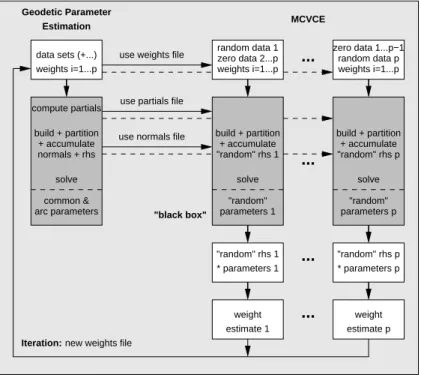
simply by zeroes. The Fig. 1 points out the principle: Af-ter step 2 (the inversion software solves from all available data sets for the gravity unknowns, given an initial weighting scheme), one has to run again the inversion for each of the pdata sets with the same normal or design matrix but with different right-hand sides X0iPiwi. Since each of these
right-hand sides consists of zeroes for p − 1 data sets, the overall numerics to be added (within one iteration of the process) is one re-computation of a full right-hand side vector, and p so-lutions of the normal equations for varying right-hand sides. Using these solutions, p data synthesis operations have to be added to obtain the p variance estimates and a new weighting scheme.
4 Numerical studies
4.1 Noise variance estimation within long-wavelength gravity field recovery from the GPS–POD
The GPS receiver aboard GOCE plays a multiple role; it en-ables a high-precision orbit determination allowing the
gra-diometer data to be processed without estimation of orbit er-rors, and it serves for recovery of the long-to-medium part of the gravity field. The POD is expected to be at the cm-accuracy level (Visser and van den IJssel, 2000).
In this study a simulated 10 days GOCE orbit solution has been used as pseudo observation set, i.e. cartesian x, y, and z coordinates in an Earth-centered quasi-inertial ref-erence frame, split up into p = 10 data sets (orbital arcs) of 1 day each. In an adjustment for gravity parameters β = (δc02, δc12, δs12, . . .)T (that is, the difference of the harmonic coefficients between the ‘true’ model OSU91a and the adopted initial model JGM-3) as well as for 10 sets of state-vector epoch parameters βi = (x, y, z, vx, vy, vz)T, i = 1 . . . 10, the partial derivatives of the satellite positions with respect to the unknowns have been obtained by numer-ical integration of the variational equations. The OSU91a model has been used complete up to degree 50 for the orbit generation. One has to note that the parameter estimation process actually has to be iterated due to linearization errors; however these errors are systematic but small for degree 50 and no re-computation of the partials was applied. Also no regularization was imposed on the estimation process. Of course, these considerations should be revised when higher resolutions will be taken into account. Simulated noise-free data and partials files, computed from the GEODYN II orbit determination software (McCarthy et al., 1993) have been kindly provided by P. Visser. A detailed description is given in (Visser et al., 2001), where this data set has been used in a comparative study on the quality of different recovery methods. At the time of writing, it is indeed expected that the variational approach will be followed in the derivation of the official ESA level–2 gravity field product from the GPS POD. We added a generated colored noise sequence to these data, whose power spectral density (PSD) model shows peaks of (2cm/1.5cm/0.8cm) at the 1cpr frequency in along/cross/radial orbit direction, and remains flat elsewhere. For the inversion, these pseudo-observed coordinates x, y, and z were assumed as uncorrelated in time as well as with respect to each other (thus both assumptions causing stochas-tic model errors), and an unknown variance component σi2 has been assigned to each orbital arc. For all experiments we assumed equal start values σi2 =(1cm)2for the first it-eration. Results are given for the estimated common gravity parameters ˆβ, expressed in terms of geoid height errors, and for the estimated variance components.
In a first simulation run, we scaled the generated noise se-quences for each arc individually by a random factor with ex-pectation one and sigma 0.5, thus simulating fluctuations of the noise level. Geoid errors and the range of the estimated variance levels are shown in Table 1. Clearly, such moder-ate noise level fluctuations have only minor influence on the gravity field solution. But nevertheless, a few iterations of MCVCE could improve the solution somewhat in terms of maximum geoid errors (being located at the polar areas due to the lack of measurements). The estimated range of vari-ances give a good validation of the simulated fluctuation.
84 J. Kusche: Noise variance estimation
use partials file
use normals file
"black box" + accumulate build + partition solve weight "random" parameters p "random" rhs p estimate p
...
...
...
MCVCE Geodetic Parameter + accumulate compute partials build + partition solve Estimation normals + rhs weights i=1...p arc parameters common &data sets (+...) use weights file
new weights file
Iteration: + accumulate build + partition solve weight "random" "random" rhs 1 parameters 1 estimate 1 weights i=1...p weights i=1...p random data 1 zero data 2...p zero data 1...p−1 random data p "random" rhs 1 * parameters 1 "random" rhs p * parameters p
...
Fig. 1. Modular use of inversion software within MCVCE software.
Table 1. Results for the first case. Noise levels vary between the
arcs with 0.5cm standard deviation Geoid errors [cm]
case max rms average estimated ˆσi[cm]
equal weights 105.3 11.0 16.2 1
1st iteration 104.3 11.1 16.4 0.8. . . 1.4
5th iteration 100.9 11.0 16.3 0.7. . . 1.7
convergence 100.3 10.9 16.2 0.6. . . 1.8
Afterwards, we repeated the same experiment but for two arcs the simulated noise level was now doubled with re-spect to the original (2cm/1.5cm/0.8cm) noise sequence, see table 2. The two ‘bad’ arcs (20% of the data!) in fact cause strongly increased geoid errors, when no downweight-ing takes place at all. After downweightdownweight-ing in the course of the MCVCE iteration, these errors are damped reasonably. 4.2 Assessing total power of noise and of signal-variance
constraints in a gradiometry-only solution
The performance of MCVCE has been investigated, in a sec-ond study, for its ability of validating the gradiometer total noise power in a full-scale simulation, complete until degree and order 300. One has to note that for this high resolution some kind of regularization is indispensible. In the present study this is achieved by introducing different Kaula-type
Table 2. Results for the first case. For two arcs the noise level has
been doubled
Geoid errors [cm]
case max rms average estimated ˆσi[cm]
equal weights 158.4 16.6 24.1 1
1st iteration 132.6 13.6 20.1 1.4 . . . 2.2
5th iteration 114.0 12.7 18.3 0.9 . . . 2.8
convergence 107.7 12.4 17.8 0.8 . . . 2.8
‘weak’ constraints for the signal power of the potential or of derivatives; ‘weak’ means that the total variance of these a priori models leaves to be determined from the analysis of the data. With other words, a variance factor for the a priori model has to estimated.
A circular orbit, almost repeat with 961 orbit revolutions during 59.8 nodal days, has been generated. The differ-ence between OSU91a and GRS80 defines the ‘true’ dis-turbing potential to be recovered. Along the orbit second radial derivatives of the disturbing potential were generated at known positions with a sampling rate of 5 seconds, which gives about one million observations. These were corrupted by a coloured noise, generated from a power spectral density function with a flat spectrum of 9 mE2/Hz between 0.005 Hz and 0.1 Hz and a 1/f2behaviour between 3.7 · 10−4Hz and 0.005 Hz. The time-wise approach was followed in the
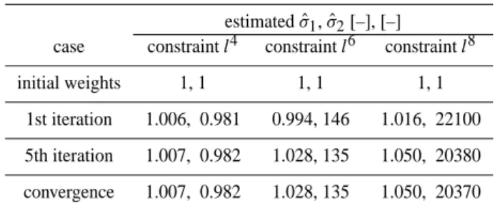
com-Table 3. Results for the second case
estimated ˆσ1, ˆσ2[–], [–]
case constraint l4 constraint l6 constraint l8
initial weights 1, 1 1, 1 1, 1
1st iteration 1.006, 0.981 0.994, 146 1.016, 22100
5th iteration 1.007, 0.982 1.028, 135 1.050, 20380
convergence 1.007, 0.982 1.028, 135 1.050, 20370
putation of the normal equations, yielding a strictly block-diagonal normal matrix. Coloured noise has been taken into account in MCVCE by replacing operations v = P u by an ARMA-filter, vn =un−Ppk=1ap,kvn−k+Pql=1bq,iun−i.
In the variance-component estimation, this filter implemen-tation can be of low order; we found p = q = 2 sufficient.
For regularization, we added Kaula–type matrices K to the normal equations; this means, with entries of order ∼ l4, l6(first order derivative regularization), or l8(second order derivative regularization). The total variance σ12of the gra-diometer observations, as well as a variance factor σ22for the signal constraint matrix, has been left open within the analy-sis for determination by MCVCE. That is, the normal equa-tions in step 2 of the algorithm of section 2 read explicitly
1 σ12(k) X0P X + 1 σ22(k) K ! ˆ β(k)= 1 σ12(k) X0P y
The geoid rms errors are of the order 16 cm for all cases, when excluding the polar areas. This reflects the observation that the quality of the gravity field solution is not very sen-sitive with respect to the choice of the regularization matrix. But looking at Table 3 we conclude that if the aim is to vali-date the gradiometer noise level, the constraint implemented in the regularization matrix should not deviate too much from the power (degree variances) of the Earth’s true gravity field. This could be expected since in the stochastic interpretation σ22K takes the role of the a priori variance–covariance ma-trix of the spherical harmonic coefficients. Ideally, ˆσ1would be estimated to 1, meaning that the a priori stochastic model that has been used both for simulation and for data analy-sis, is perfectly validated. Small deviations may be related to imperfections in the filter design.
5 Discussion
A method has been proposed for validating the variance lev-els for the different GOCE observation types, and based on this, for the determination of an optimal weighting scheme. The method treats all observations as input within a joint pa-rameter estimation, thus without leaving certain data out for independent validation. It relies basically on the well-known and powerful method of variance-component estimation, re-cast in a Monte Carlo framework. As a consequence, it can
be used without re-coding existing L2 inversion software. However, numerical studies so far concern only very specific test cases, and experience has still to be gained. A point of concern might be that (multiplicative) variance components can only account for the total power of a particular stochas-tic model, relying on the a priori structure of the variance-covariance matrix for this type of observations. In the present form it is therefore not possible to relate an estimated vari-ance level to a specific bandwidth in a given power spectral density (PSD) model; that is to improve the PSD model it-self apart from a simple re-scaling. To this end, the joint estimation scheme would have to be further extended for co-variance components, each of which facilitating an additional degree of freedom in the (time-wise) correlation structure of an observation type. However, whereas the theory and appli-cation of variance-covariance-component estimation is well-investigated, efficient Monte Carlo type algorithms still have to be developed.
Acknowledgements. We thank Pieter Visser from DEOS for
pro-viding us with simulated GOCE orbit data and partials files. J.-P. Barriot and an anonymous reviewer gave helpful remarks that im-proved the quality of the manuscript.
References
ESA: Gravity Field and Steady-State Ocean Circulation Mission. Reports for Mission Selection, ESA SP-1233(1), ESTEC, No-ordwijk, 1999.
Grafarend, E. W., Kleusberg, A., and Schaffrin, B.: An introduc-tion to the variance-covariance component estimaintroduc-tion of Helmert type, Zeitschrift f¨ur Vermessungswesen, 105, 161–180, 1980.
Koch, K.-R.: Bayesian Inference with Geodetic Applications,
Springer, Berlin, 1990.
Koch, K.-R. and Kusche, J.: Regularization of geopotential deter-mination from satellite data by variance components, J. Geodesy, 76, 259–268, 2002.
Koop, R., Bouman, J., Schrama, E. J. O., and Visser, P.: Calibration and error assessment of GOCE data, in: Vistas for Geodesy in the New Millenium, (Eds) Adam, J. and Schwarz, K.-P., Springer, 2002.
Kusche, J.: A Monte Carlo Technique for Weight Estimation in Satellite Geodesy, J. Geodesy, 76, 641–652, 2003.
McCarthy, J. J., Rowton, S., Moore, D., Pavlis, D. E., Luthcke, S. B., and Tsaoussi, L. S.: GEODYN II Systems Descrip-tion, NASA Goddard Space Flight Center, Greenbelt, Maryland, 1993.
Visser, P. and van den IJssel, J.: GPS–based precise orbit determi-nation of the very low Earth-orbiting gravity mission GOCE, J. Geodesy, 74, 590–602, 2000.
Visser, P., van den IJssel, J., Koop, R., and Klees, R.: Exploring gravity field determination from orbit perturbations of the euro-pean gravity mission GOCE, J. Geodesy, 75, 89–98, 2001.