Some aspects of the geomagnetic response to solar wind pressure variations: a case study at low and middle latitudes

HAL Id: hal-00317423

https://hal.archives-ouvertes.fr/hal-00317423

Submitted on 14 Jun 2004

HAL is a multi-disciplinary open access

archive for the deposit and dissemination of

sci-entific research documents, whether they are

pub-lished or not. The documents may come from

teaching and research institutions in France or

abroad, or from public or private research centers.

L’archive ouverte pluridisciplinaire HAL, est

destinée au dépôt et à la diffusion de documents

scientifiques de niveau recherche, publiés ou non,

émanant des établissements d’enseignement et de

recherche français ou étrangers, des laboratoires

publics ou privés.

pressure variations: a case study at low and middle

latitudes

U. Villante, P. Di Giuseppe

To cite this version:

U. Villante, P. Di Giuseppe. Some aspects of the geomagnetic response to solar wind pressure

varia-tions: a case study at low and middle latitudes. Annales Geophysicae, European Geosciences Union,

2004, 22 (6), pp.2053-2066. �hal-00317423�

Annales Geophysicae (2004) 22: 2053–2066 SRef-ID: 1432-0576/ag/2004-22-2053 © European Geosciences Union 2004

Annales

Geophysicae

Some aspects of the geomagnetic response to solar wind pressure

variations: a case study at low and middle latitudes

U. Villante and P. Di Giuseppe

Dipartimento di Fisica, Universit`a and Area di Ricerca in Astrogeofisica, L’Aquila, Italy

Received: 16 April 2003 – Revised: 25 February 2004 – Accepted: 1 March 2004 – Published: 14 June 2004

Abstract. We examined geomagnetic field observations at low and middle latitudes in the Northern Hemisphere during a 50-min interval (12 May 1999), characterized by a com-plex behaviour of the solar wind dynamic pressure. For the entire interval, the aspects of the geomagnetic response can be organized into four groups of events which show common characteristics for the H and D components, respectively. The correspondence between the magnetospheric field and the ground components reveals different aspects of the ge-omagnetic response in different magnetic local time (MLT) sectors. For the H component, the correspondence is highly significant in the dusk and night sectors; in the dawn and prenoon sectors it shows a dramatic change across a separa-tion line that extends approximately between (6 MLT, 35◦₎ and (13 MLT, 60◦_{). For the D component, the} correspon-dence has significant values in the dawn and prenoon re-gions. We propose a new approach to the experimental data analysis which reveals that, at each station, the magneto-spheric field has a close correspondence with the geomag-netic field projection along an axis (M1) that progressively rotates from north/south (night events) to east/west orienta-tion (dawn events). When projected along M1, the geomag-netic signals can be interpreted in terms of a one-dimensional pattern that mostly reflects the field behaviour observed at geostationary orbit. Several features appear more evident in this perspective, and the global geomagnetic response to the SW pressure variations appears much clearer than in other representations. In particular, the MLT dependence of the ge-omagnetic response is much smaller than that one estimated by previous investigations. A clear latitudinal dependence emerges in the dusk sector. The occurrence of low frequency waves at ∼2.8 mHz can be interpreted in terms of global magnetospheric modes driven by the SW pulse. This event occurred in the recovery phase after the day the SW almost disappeared (11 May 1999): in this sense our results suggest a rapid recovery of almost typical magnetospheric conditions

Correspondence to: U. Villante

(umberto.villante@aquila.infn.it)

soon after a huge expansion. Overshoot amplitudes, greater than in other cases, are consistent with a significant reduction of the ring current.

Key words. Magnetospheric physics (Solar wind-magnetosphere interaction; Current systems; Magneto-spheric configuration and dynamics)

1 Introduction

An interesting aspect of the relationships occurring between the solar wind (SW) and the Earth’s magnetosphere is rep-resented by the geomagnetic response to variations of the SW parameters. In particular, the Earth’s arrival of SW structures, characterized by sudden variations of the dynamic pressure (1Psw) is known to be related to impulsive vari-ations of the geomagnetic field (SIs). SIs mainly consist of sharp variations of the north/south component (H ); their amplitude (1H ) is roughly proportional to 1(P1/2sw), with a coefficient that typically ranges from 13 to 34 nT/(nPa)1/2 (Siscoe et al., 1968; Su and Konradi, 1975; Nishida, 1978). Similarly, the expansion of the magnetosphere, during in-tervals of reduced SW pressure produces, at low latitudes, an H decrease that mostly reflects the magnetospheric field waveform (Araki and Nagano, 1988). Specific attention has been addressed in the scientific literature to the local time dependence of the geomagnetic response. Statistical anal-ysis revealed that the asymptotic response of the H com-ponent shows at low latitudes (15◦_–30◦_{) a weak MLT} de-pendence (MLT being the magnetic local time), with maxi-mum values around local noon, minimaxi-mum values around mid-night, and an average value of ∼16.5 nT/(nPa)1/2(Russell et al., 1992, 1994a). At subauroral latitudes (∼54◦–58◦), the asymptotic response shows a different pattern, with strongly depressed (and even negative) values in the morning, and enhanced values in the afternoon (∼30 nT/(nPa)1/2; Russell and Ginskey, 1995). Previous analysis of the latitudinal de-pendence of the asymptotic variation (H component) showed

Table 1. List of geomagnetic observatories with geographic and

corrected geomagnetic coordinates.

Geographic Corr. Geomagnetic

Station Lat. Long. Lat. Long.

ABG 28.62 72.87 22.81 145.32 AQU 42.38 13.32 36.28 87.51 BDV 49.08 14.02 44.44 89.62 BEL 51.84 20.80 47.55 96.23 BFE 55.63 11.67 52.07 89.69 BMT 40.30 116.20 34.46 188.68 BOU 40.14 254.76 49.07 319.52 BSL 30.40 270.60 41.43 340.62 CLF 48.02 2.27 43.50 79.50 DLR 29.49 259.08 38.90 326.22 ESK 55.30 356.80 52.71 77.52 FRD 38.21 282.63 49.22 357.64 FRN 37.09 240.28 43.04 303.51 FUR 48.17 11.28 43.39 87.05 HAD 51.00 355.50 47.69 74.93 HLP 54.61 18.82 50.67 95.34 HRB 47.86 18.19 42.99 92.93 IRT 52.17 104.45 47.19 177.20 KAK 36.23 140.18 29.20 211.65 LER 60.10 358.80 57.99 81.27 LNP 35.00 121.20 28.72 193.42 LOV 59.34 17.82 55.88 96.25 MMB 43.91 144.19 37.02 215.31 NCK 47.78 16.43 42.90 91.38 NEW 48.26 242.88 54.96 303.22 NGK 52.07 12.68 47.96 89.33 NUR 60.51 24.66 56.87 102.46 OTT 45.40 284.45 56.05 0.89 SJG 20.00 293.88 30.00 10.51 SPT 39.55 4.35 32.38 79.30 STJ 47.60 307.32 53.80 31.19 SUA 45.32 26.25 40.22 99.67 THY 43.25 17.89 37.38 91.70 TUC 32.25 249.17 39.88 314.37 VIC 48.52 236.58 53.85 296.01 WNG 53.74 9.07 50.03 86.87

a negative gradient between ∼5◦_–50◦_{, both in diurnal and} nocturnal sectors (Le et al., 1993; Russell et al., 1994a, b); more recently, however, Francia and Lepidi (2002) found a positive gradient between ∼36◦–65◦, in the afternoon sec-tor. On the other hand, since early investigations (Matsushita, 1962; Nishida and Jacobs, 1962) different waveforms of the

Hcomponent were detected at different stations. Nowadays, the current understanding suggests a complex scenario that relates the H waveform to the combined effects of the mag-netopause and ionospheric current systems; the D variation (D being the east/west component) is basically related to ionospheric contributions (Araki, 1994; Tsunomura, 1998).

In the present paper we discuss several aspects of the geo-magnetic field variations (observed at a number of stations between low and middle latitudes in the Northern Hemi-sphere, Table 1) during a 50-min interval. This period is characterized by a complex behaviour of the SW dynamic pressure (i.e. a rarefaction region, with imbedded minor am-plitude variations, followed by a sharp increase). This event occurred on 12 May 1999, 15:30–16:20 UT, i.e. in the re-covery phase after the day the SW almost disappeared (Far-rugia et al., 2000; Fairfield et al., 2001; Le et al., 2000; Papitashvili et al., 2000; Rostoker, 2000; Terasawa et al., 2000). After a prolonged interval of extremely low values (below 1 cm−3), the density started to recover after 11 May at ∼22:00 UT, reaching ∼20 cm−312 on May at ∼18:00 UT; in the period of interest, the number density was ∼7.5 cm−3, and the bulk velocity ∼420 km/s. We examined the rela-tions between the SW/magnetospheric structures and ground measurements. We focused specific attention on the corre-spondence between the magnetospheric field (B) observed at geostationary orbit in the noon quadrant and geomagnetic field measurements at different sites. Following previous in-vestigations (Russell et al., 1992, 1994a, b; Le et al., 1993; Russell and Ginskey, 1995; Francia et al., 1999, 2001), we carefully examined the aspects of the MLT and latitudinal dependence of the asymptotic response.

Separate analysis of the H and D component provided interesting results. Indeed, the correspondence between B and H is highly significant in the dusk and night sectors. In the dawn and prenoon regions it shows a dramatic vari-ation across an oblique separvari-ation line that extends approx-imately between (06:00 MLT, 35◦) and (13:00 MLT, 60◦). Conversely, the correspondence between B and D has sig-nificant values in the dawn and prenoon sectors. Obviously, these features simply reflect the different role of the current systems at different sites. They suggest, however, that the usual analysis of the H component alone might provide am-biguous estimates of the amplitude and modulation of the geomagnetic response. We then propose a new approach to the experimental data analysis in which the aspects of the geomagnetic response at each station are investigated after determining the direction of maximum correlation between

B and the ground field. This new approach reveals that the major characteristics of the low-and middle-latitude sig-nals can be interpreted in terms of a one-dimensional pattern that mostly reflects the field observed at geostationary orbit.

U. Villante and P. Di Giuseppe: Some aspects of the geomagnetic response to solar wind pressure variations 2055 Several features appear more evident in this perspective, and

the global geomagnetic response to the SW pressure vari-ations appear much clearer than in other representvari-ations. In particular, the MLT dependence of the geomagnetic response is much smaller than that one estimated by previous analysis, and its latitudinal dependence emerges only in the dusk and night sectors.

2 The correspondence between interplanetary and magnetospheric observations

The interplanetary (Wind), magnetospheric (Goes 8, MLT=UT–5.05) and geomagnetic observations (L’Aquila (AQ), Italy, corrected latitude ∼36.2◦, MLT=UT+1.37) are compared in Fig. 1a for the time interval 09:00–24:00 UT on 12 May. At that time Wind was located at a radial geocentric distance of ∼44 Re. After ∼12:00 UT, the SW flow is charac-terized by explicit variations of the dynamic pressure which find correspondence in the magnetospheric (magnitude B, and Bz component) and ground field (H component). A preliminary comparison between 1Psw measurements from ACE (∼225 Re) and Wind showed a close correspondence for an average delay time of ∼48±3 min. It implies a radial propagation speed of ∼400±25 km/s, which is consistent with the average SW velocity (418±10 km/s). On the other hand, the best correspondence between Wind (1(P1/2sw))and Goes 8 (1B) (ρ=0.90, 10:00–14:00 MLT, ρ being the corre-lation coefficient) is obtained for a delay time of ∼12±3 min, i.e. somewhat longer than expected (∼10 min) for a constant, 400 km/s transit speed (Fig. 1b). This result suggests an av-erage speed of travelling disturbances within magnetosheath appreciably lower than in the interplanetary medium; never-theless, the uncertain dimensions of the extended magneto-sphere (Fairfield et al., 2001) do not allow any quantitative evaluation of the propagation speed. The results of Fig. 1b also show a much smaller correspondence in the morning and afternoon quadrant (ρ=0.52, 6–10 MLT; ρ=0.15, 14:00– 18:00 MLT).

A major pressure variation was observed by Wind between

∼15:17–16:07 UT. This structure is more carefully compared with the magnetospheric field observations in Fig. 1c. The step-like variation (1(P1/2sw) ∼0.87 (nPa)1/2) is preceded by a longer term (∼15 min) rarefaction region with some smaller pressure variations. Both the declining and the as-cending structures find clear correspondence in the magne-tospheric field observations. These observations also con-firm that the magnetospheric response in the noon quad-rant is much more explicit than in the dawn and dusk sec-tors (Kokubun, 1983; Kuwashima and Fukunishi, 1985; Sastri et al., 2001): indeed, a sharp peak-to-peak varia-tion of ∼19.2 nT was observed by Goes 8 (∼11:00 MLT, with a global rising time 1T of ∼10 min), while the same variation was remarkably smaller (∼13.8 nT) and smoother (1T ∼16 min) at Goes 10 position (∼07:00 MLT). When related to 1(P1/2sw), Goes 8 observations suggest a nor-malized magnetospheric response of ∼22.4 nT/(nPa)1/2 in

5 10 B (nT) (a) 12 15 18 21 2 4 P_SW (nPa) UT 100 150 Bz_G8 (nT) 6 9 12 15 18 100 150 B_G8 (nT) MLT 12 15 18 21 24 −20 0 20 H_AQ (nT) MLT 6 8 10 12 14 16 18 −12 −6 0 6 ∆ BG8 (nT) Goes 8 MLT 12 14 16 18 20 22 −0.8 −0.4 0 0.4 ∆ (P SW ) 1/2 (nPa) 1/2 UT (b) 0.4 0.6 0.8 1 1.2 1.4 1.6 1.8 (PSW ) 1/2 (nPa 1/2 ) 1530 1540 1550 1600 1610 UT −15 −10 −5 0 5 10 ∆ B (nT) (c) Goes 8 MLT = UT−5.05 Goes 10 MLT = UT−9.05 WIND

Fig. 1. (a) A comparison between Wind, Goes 8 and ground

obser-vations at L’Aquila for 12 May 1999 (09:00–24:00 UT). From the top: B is the IMF intensity, PSW the SW dynamic pressure, BzG8 the north-south component of the magnetospheric field in GSM co-ordinates, BG8the total magnetospheric field, and HAQthe north-south component of the geomagnetic field. Magnetospheric and ground observations are organized in Magnetic Local Time (MLT).

(b) The correspondence between the 3-min averages of the square

root of the SW pressure (solid line) and the magnetospheric field (dashed line) (11:00–23:00 UT). SW observations have been de-layed by 12 minutes. In both cases the long-term variations have been removed. On the top scale the MLT at Goes 8. (c) A com-parison between the square root of the SW pressure (solid line) and the magnetospheric field from Goes 8 (dashed line), and Goes 10 (dotted line).

0 4 8 12 16 20 MLT 20° 30° 40° 50° 60° Λ H 20 nT

1

1

2

3a

3b

1

1

2

3a

3b

Fig. 2. Geomagnetic field observations (1-min averages) at stations located at different MLT and latitude 3 in the Northern Hemisphere

for the time interval 15:35–16:05 UT. H component is in the upper panel and D component in the lower panel. Ground observations are organized in four groups, 1, 2, 3a, and 3b, according to the similar behavior observed in the geomagnetic field components. The MLT of GOES satellites (G8 and G10) is marked with arrows at the bottom of both panel.

U. Villante and P. Di Giuseppe: Some aspects of the geomagnetic response to solar wind pressure variations 2057 1530 1550 1610 UT (2348, 28.7°) A C E F (2330, 34.5°) Goes 8 10 nT H

(a)

(b)

Fig. 3. (a) The magnetic field observations (H component) for two different MLT sectors in group 1. (b) The magnetic field observations

for a single MLT strip in group 2. Left plot: H component, right plot: D component. In the bottom trace of each panel the magnetospheric field from Goes 8.

the noon quadrant. Correspondingly, the asymptotic vari-ation at Goes 8 and Goes 10 is, respectively, ∼16.0 nT (∼18.7 nT/(nPa)1/2), and ∼12.7 nT (∼14.6 nT/(nPa)1/2). Similarly, the initial negative variation has a total excursion of ∼ –8.2 nT and ∼ –4.5 nT at Goes 8 and Goes 10. The first ground SI appearance is detected approximately within 1 min after the magnetospheric field variation (Nishida, 1978): this observation suggests an average propagation velocity of

as-sociated disturbances in the inner magnetosphere of at least

∼600 km/s, i.e. consistent with current estimates of the fast mode velocity (Farrugia et al., 1989; Araki, 1994; Araki et al., 1997). As we show in the following, ground observations in any time sector mostly reflect the magnetospheric field be-haviour in the noon quadrant.

1530 1550 1610 UT (0858, 38.9°) (0953, 41.4°) H Goes 8 10 nT

(a)

(b)

Fig. 4. The same as in Fig. 3b for group 3a (a) and 3b (b).

3 An analysis of the geomagnetic response

A joint analysis of the morphological aspects of H and D for the entire 50-min interval (15:30–16:20 UT, 1-min averages, Fig. 2) shows a clear organization of ground observations in groups of events with different characteristics (Matsushita, 1962; Nishida and Jacobs, 1962). This analysis also makes explicit that a clear variation of the geomagnetic field be-haviour (which mostly influences the H component) occurs across a separation line that extends approximately between (06:00 MLT, 35◦_{) and (13:00 MLT, 60}◦_{). These different} aspects are shown more clearly in Figs. 3 and 4, where ob-servations are organized in narrow MLT strips. Here points A, C, E, and F identify the major field variations which have different amplitudes in different regions (and even disappear in some cases). Namely, A (15:36–15:39 UT) identifies the peak value before the main decrease; C (15:47–15:48 UT), the peak enhancement occurring during depressed magneto-spheric field conditions; E (15:48–15:49 UT), the minimum value before the main variation; F (15:56–15:58 UT), the overshoot field (i.e. the peak value that precedes the asymp-totic variation, Russell and Ginskey, 1993); we also show, for

comparison, in the bottom trace of each panel, the B field at Goes 8 position. The principal characteristics of the different groups can be briefly summarized as follows.

Group 1. In the midnight sector (22:00–01:00 MLT, Fig. 3a) the geomagnetic field trace is characterized by ex-plicit variations of the H component (D only shows small amplitude fluctuations, Fig. 2). These variations mostly re-flect the magnetospheric field trace. No clear evidence for the C enhancement is detected in this sector. As for other cases, significant differences of the geomagnetic response appear for small MLT separation. Indeed, at ∼29◦ the peak varia-tion (HF – HE∼24.2 nT) at 23:48 MLT is ∼50% larger than one hour later (∼16.3 nT, 00:53 MLT).

Group 2. In the dusk sector (16:00–19:00 MLT, Fig. 3b) the traces of both components are much more structured. A clear C enhancement precedes by several minutes a sharp overshoot (F). Both C and F (as well as the entire pattern) show a general tendency to increase with increasing latitude and find poor correspondence in the magnetospheric field. The most significant H variations correspond to simultane-ous variations of the D component of opposite sign: indeed,

U. Villante and P. Di Giuseppe: Some aspects of the geomagnetic response to solar wind pressure variations 2059 0 4 8 12 16 20 LT 20° 30° 40° 50° 60° .98 .98 .98 .98 .95 .98 .97 .98 .97 .94 .95 .90 .94.96 .96 .69 .96 .96.97 .97 .95 .94 .95 .11 .69 .95 .91 .91 .91 .73 −.15−.31 .93 −.24 .93 .93 Λ ρ_BH 0 4 8 12 16 20 LT 20° 30° 40° 50° 60° −.77 −.18 .65 .36 −.88 .36 −.84 −.09 −.81 .92 .87 .89 −.61 −.77−.65 .79 −.90 −.85−.88 −.40 −.83 −.89 −.74 .86 .88 −.81−.77 −.73 −.83 .68 .64.73 −.87 .89 −.86 −.88 Λ ρ_BD 0 4 8 12 16 20 LT 20° 30° 40° 50° 60° .98 .98 .98 .98 .96 .98 .97 .98 .97 .95 .95 .92 .96 .95 .96 .82 .96 .96.97 .97 .96 .94 .96 .86 .91 .95.91 .92 .91 .87 .65.75 .94 .89 .94 .95 Λ ρ_VM1 0 4 8 12 16 20 LT 20° 30° 40° 50° 60° .98 .98 .98 .98 .95 .98 .97 .98 .97 .94 .95 .90 .94.96 .96 .69 .96 .96.97 .97 .95 .94 .95 .11 .69 .95 .91 .91 .91 .73 −.15−.31 .93 −.24 .93 .93 Λ ρ_BH 0 4 8 12 16 20 LT 20° 30° 40° 50° 60° −.77 −.18 .65 .36 −.88 .36 −.84 −.09 −.81 .92 .87 .89 −.77−.61 −.65 .79 −.90 −.85−.88 −.40 −.83 −.89 −.74 .86 .88 −.81−.77 −.73 −.83 .68 .64.73 −.87 .89 −.86 −.88 Λ ρ_BD 0 4 8 12 16 20 LT 20° 30° 40° 50° 60° .98 .98 .98 .98 .96 .98 .97 .98 .97 .95 .95 .92 .96 .95 .96 .82 .96 .96.97 .97 .96 .94 .96 .86 .91 .95.91 .92 .91 .87 .65.75 .94 .89 .94 .95 Λ ρ_VM1 0 4 8 12 16 20 LT 20° 30° 40° 50° 60° .98 .98 .98 .98 .95 .98 .97 .98 .97 .94 .95 .90 .94.96 .96 .69 .96 .96.97 .97 .95 .94 .95 .11 .69 .95 .91 .91 .91 .73 −.15−.31 .93 −.24 .93 .93 Λ ρ_BH 0 4 8 12 16 20 LT 20° 30° 40° 50° 60° −.77 −.18 .65 .36 −.88 .36 −.84 −.09 −.81 .92 .87 .89 −.77−.61 −.65 .79 −.90 −.85 −.88 −.40 −.83 −.89 −.74 .86 .88 −.81−.77 −.73 −.83 .68 .64.73 −.87 .89 −.86 −.88 Λ ρ_BD 0 4 8 12 16 20 LT 20° 30° 40° 50° 60° .98 .98 .98 .98 .96 .98 .97 .98 .97 .95 .95 .92 .96 .95.96 .82 .96 .96.97 .97 .96 .94 .96 .86 .91 .95.91 .92 .91 .87 .65.75 .94 .89 .94 .95 Λ ρ_VM1

Fig. 5. The correlation coefficient between the magnetospheric field B and the geomagnetic field elements for the time interval 15:30–

16:20 UT. Top panel: correlation with the H component (ρBH); central panel: correlation with the D component (ρBD); bottom panel: correlation with the field projection along the maximum correlation axis (ρV M1).

2060 U. Villante and P. Di Giuseppe: Some aspects of the geomagnetic response to solar wind pressure variations 0° 20° 40° 60° 2:00 14:00 4:00 16:00 6:00 18:00 8:00 20:00 10:00 22:00 12:00 0:00 (a) 0° 20° 40° 60° 2:00 14:00 4:00 16:00 6:00 18:00 8:00 20:00 10:00 22:00 12:00 0:00 (b) 20° 40° 60° 2:00 14:00 4:00 16:00 18:00 8:00 20:00 10:00 22:00 12:00 0:00 0° 20° 40° 60° 2:00 14:00 4:00 16:00 6:00 18:00 8:00 20:00 10:00 22:00 12:00 0:00 (b)

Fig. 6. (a) The orientation of the maximum correlation axis (M1) between the magnetospheric field B and the geomagnetic field for the

entire set of ground stations. (b) The equivalent ionospheric current system superimposed to the current system proposed by Nishida (1968). The length of the arrows is proportional to the asymptotic variation.

D shows negative peak values (A), negative C variations, deep minimum values (F), and a general tendency to decrease after the main variation.

Group 3. Unlike dusk and night events, dawn and prenoon events (07:00–13:00 MLT, Fig. 4) are characterized by a D behaviour which basically reflects the magnetospheric field, with a similar pattern on both sides of the separation line (Fig. 2). Nevertheless, a dramatic amplitude reduction oc-curs at later MLTs: for example, the peak-to-peak variation is

∼20.9 nT at (07:28 MLT, 43◦) and ∼13.7 nT at (09:53 MLT, 41.4◦). Conversely, striking differences emerge in the H component, even for small MLT separation. Indeed, while below the separation line (group 3a), the H component still reflects the magnetospheric field, above this line (group 3b) it rather shows an irregular behaviour with a dominant positive-then-negative variation which is more explicit at ∼55◦.

A simple analysis of the correlation coefficient between B and the geomagnetic field components for the entire 50-min interval (ρBH,ρBD, Fig. 5) reinforces the conclusions of the previous paragraph. Indeed, ρBH, which is high (>.90) in the dusk sector, has maximum values (>.97) in the midnight sector. Moreover, greater ρBH values are typically observed at lower latitudes, as expected for a smaller influence of the ionospheric current system. In the dawn and prenoon sec-tors, significant differences occur across the separation line: indeed, below this line (i.e. at later MLTs), ρBHhas high val-ues; conversely, above this line, H is not correlated to B. The

ρBDvalues confirm a different MLT dependence: it has sig-nificant values in the dawn and prenoon sectors while show-ing some evidence for an anticorrelation in the dusk sector.

We adopted a different approach to the experimental data analysis to make more clear the aspects of the correspon-dence between the magnetospheric and ground field. For this scope, we determined the direction (V-axis) associated with the maximum excursion of the magnetospheric field in the noon quadrant (it is found in the meridian plane, with a strongly dominant contribution along Zsm). We then identi-fied at each station the direction (M1-axis) of maximum cor-relation (for the entire 50-min interval) between the magne-tospheric field projection along V and the geomagnetic field projection along M1, evaluating the correlation coefficient (ρV M1)between the two fields at steps of 1◦. The results

of this analysis (Figure 5, bottom panel) are very interest-ing: indeed, they reveal a highly significant correspondence between the magnetospheric and the ground field along M1 in the entire latitudinal and MLT range. No dramatic varia-tion of the correlavaria-tion coefficient occurs in this case across the separation line. Nevertheless, the smaller ρV M1, with

minimum values at (∼07:00 MLT, ∼55◦), suggest a greater influence of ionospheric contributions at earlier MLTs.

In addition, we also determined, at steps of 1◦_{, the} direc-tion (M2) of maximum asymptotic variadirec-tion of the ground field. For this scope we considered, as the initial level, the 5-min averages of the geomagnetic signals before the SI and, as the final level, the new steady state (15-min average) ob-served 15 min after the SI onset (different choices of the av-eraging intervals do not significantly influence the results of our analysis). As a matter of fact, M1 and M2 typically coin-cide: it confirms that at low and middle latitudes the ground variations mostly reflect, with different amplitude and orien-tation, the magnetospheric field variations. Nevertheless, in

U. Villante and P. Di Giuseppe: Some aspects of the geomagnetic response to solar wind pressure variations 2061 (1808, 55.9o) θ = 336o Group 2 A C E F (1256, 53.8o) θ = 40o Group 3a A C E F (0733, 55.0o) θ = 101o Group 3b A C E F 10 nT (2249, 47.2o) θ = 354o Group 1 (1804, 50.7o) θ = 336o (1052, 49.2o) θ = 73o (0834, 49.1o) θ = 87o (0103, 37.0o) θ = 0o (1824, 40.2o) θ = 346o (0953, 41.4o) θ = 58o (0728, 43.0o) θ = 68o (2348, 28.7o) θ = 359o (1657, 32.4o) θ = 328o (1143, 30.0o) θ = 4o (2101, 22.8o) θ = 351o

Fig. 7. A summary of the characteristics of the ground response along the M1 axis.

agreement with previous conclusions, small angular separa-tions between M1 and M2 are observed at ∼7 MLT, ∼55◦, confirming a more significant effect of ionospheric currents. The orientation of M1 axis (Fig. 6a) shows an explicit and regular MLT dependence: it is mostly along H in the night sector; it rotates westward (10◦_–30◦_{) in the dusk sector; it} is progressively closer to D with increasing latitude in the dawn and prenoon sectors. However, at (∼12 MLT, 30◦) M1 is newly oriented along H . Assuming that the field perturba-tions are generated by a horizontal current layer in the iono-sphere, the orientation of the equivalent current system can be inferred by a 90◦rotation of M1 (Fig. 6b). Obviously, the small latitudinal range does not allow for conclusions on the entire current system. However, the inferred currents show a general correspondence with a basic two vortex pattern as

that proposed by Nishida (1968). Tentatively, we would also suggest that a closer agreement between model and observa-tions might be obtained, translating the focus of the afternoon vortex by several degrees toward earlier MLTs; nevertheless, night observations suggest in the dark sector an extension of the vortex system to low latitudes smaller than in other cases. Figure 7 shows, for different latitudinal strips, some ex-amples of the geomagnetic field trace along M1. It reveals, much better than other representations, that a similar one-dimensional pattern now emerges in any time sector (indeed, significant signals perpendicular to M1 occur only in some cases in the dawn sector). This pattern clearly reflects, from low to middle latitudes, the main aspects of the magneto-spheric field trace. Nevertheless, at (0733, 55◦; 0834, 49◦) the long-term decrease after the peak value reveals a more

2 2.5 3 3.5 4 0 10 20 30 40 50 60 70 mHz PSD (nT 2 /Hz) 16 − 19 MLT 2 2.5 3 3.5 4 0 0.5 1 1.5 2 2.5 mHz PSD (nT 2 /Hz)

(a)

(b)

Fig. 8. (a) Spectral analysis for the time interval 16:00–16:20 UT

for stations located in the dusk sector (16:00–19:00 MLT). (b) The same for Goes 8 and Goes 10.

persistent ionospheric contribution. Independent of orien-tation, the global pattern, for comparable latitudes, shows maximum amplitude (and steeper variation) in the dusk tor; it progressively decreases in the midnight and dawn sec-tors, reaching minimum values in the prenoon quadrant. Al-though with different relevance, the additional A through F elements appear in any time sector, and are less significant below ∼40◦_.

Our representation may also be useful for a more definite comparison with theoretical models. For example, the effects of the Chapman-Ferraro current have been often evaluated in terms of a step-like H signal decreasing with increasing latitude (Araki, 1994). Our results suggest a more complex scenario in which noon observations are characterized by an almost constant step-like response that assumes different ori-entations at different latitudes, while the H variation detected in the dusk sector shows a positive latitudinal gradient which is in conflict with the decrease expected for the effects of the magnetopause current alone.

Dusk observations are characterized by sharp over-shoots. Their amplitudes (increasing with latitude) over-come the asymptotic variations by a factor between ∼1.3

and ∼2.0, and are much greater (∼70 nT/nPa1/2at ∼53◦_;

∼28 nT/nPa1/2 close to midnight at ∼29◦_{) than those} esti-mated by previous analysis (∼18 nT/nPa1/2at low latitudes; between ∼17.4 nT/nPa1/2and ∼22.5 nT/nPa1/2at ∼36◦; 50– 55 nT/nPa1/2at 54◦–58◦; Russell and Ginskey, 1993; Francia et al., 2001; Russell and Ginskey, 1995). We determined the direction of the maximum overshoot fields and found them to be parallel to M1. This feature suggests that one inter-prets the overshoot field in terms of a strengthening of the same current system related to the main variation (Russell and Ginskey, 1995). Some evidence for an overshoot struc-ture with similar characteristics is observed in the night sec-tor, while it almost disappears in the noon quadrant.

The overshoot peak is followed by large amplitude, almost regular fluctuations that appear in phase at each station and persist for a few cycles. This mode appears in the dusk sector, more clearly above ∼50◦_{, and rapidly decreases below ∼40}◦ (Fig. 7). The spectral analysis (Fig. 8a) shows that these fluc-tuations consist of a dominant mode at an approximately con-stant frequency (∼2.8 mHz). It is interesting to note that this peak has correspondence in the power spectrum of the Bz component in the noon quadrant (Fig. 8b, Goes 8); it shows, indeed, a power enhancement which has approximately the same amplitude as in the low latitude ground spectra. Con-versely, Goes 10 observations do not show any power en-hancement in the early morning hours. Likely, these fluctua-tions might be related to the low frequency modes at discrete frequencies (∼1.1, 1.7, 2.3, 2.8, 3.7 mHz) that have been ob-served from low to high-latitudes and interpreted in terms of ground signatures of magnetospheric cavity/waveguide modes (Kivelson and Southwood, 1985, 1986; Samson et al., 1992; Walker et al., 1992; Villante et al., 2001, 2003). On the other hand, in agreement with present results, recent investigations proposed much clearer evidence for power en-hancements at selected frequencies in the afternoon sector and during higher pressure SW conditions; as a consequence, the onset of these fluctuations was related to the Earth’s ar-rival of higher pressure corotating SW structures impinging on the postnoon magnetosphere (Villante et al., 2001, 2003). As previously stated, the general aspects of the asymptotic variation have been currently investigated considering the ge-omagnetic response of the H component approximately 10 min after the peak response (Russell et al., 1992, 1994a, b; Russell and Ginskey, 1995; Francia et al., 2001). In order to allow for a comparison with previous investiga-tions, we conducted a similar analysis considering the dif-ference between the 10-min average, 16:05–16:15 UT, and HE. As shown in the top panel of Fig. 9, this asymp-totic response has the highest values in the dusk sector (∼21–31 nT/(nPa)1/2, above ∼40◦), where it shows a gen-eral, although irregular, tendency to increase with increas-ing latitude (Tsunomura, 1998); conversely, in the dawn and prenoon sectors, it is small for group 3a events and becomes negligible, or even negative, for group 3b events. Although with few observations, our results seem to suggest approxi-mately the same pattern at ∼30◦, where the noon response (∼11 nT/(nPa)1/2)is appreciably smaller than the midnight

U. Villante and P. Di Giuseppe: Some aspects of the geomagnetic response to solar wind pressure variations 2063 0 4 8 12 16 20 MLT 20° 30° 40° 50° 60° 17.7 20.6 15.4 11.2 16.3 24.1 18.3 20.5 23.4 9.9 8.3 22.3 6.5 23.9 22.4 4.2 21.8 21.6 23.2 26.1 30.7 25.2 29.7 0.8 2.7 34.7 30.3 34.0 35.8 6.6 −0.8−2.1 32.3 −5.7 37.1 35.4 Λ Asymptotic variation (H) 0 4 8 12 16 20 MLT 20° 30° 40° 50° 60° 17.9 20.6 15.6 11.2 19.3 24.1 20.1 20.5 25.1 15.0 14.8 23.0 12.2 25.4 23.8 11.4 23.9 24.7 24.6 26.2 32.0 28.3 30.9 15.4 9.3 36.8 33.2 35.2 39.7 8.6 9.011.7 35.3 15.4 40.2 38.3 Λ Asymptotic variation (M1) (a) 0 4 8 12 16 20 MLT 20° 30° 40° 50° 60° 17.7 20.6 15.4 11.2 16.3 24.1 18.3 20.5 23.4 9.9 8.3 22.3 6.5 23.9 22.4 4.2 21.8 21.6 23.2 26.1 30.7 25.2 29.7 0.8 2.7 34.7 30.3 34.0 35.8 6.6 −0.8−2.1 32.3 −5.7 37.1 35.4 Λ Asymptotic variation (H) 0 4 8 12 16 20 MLT 20° 30° 40° 50° 60° 17.9 20.6 15.6 11.2 19.3 24.1 20.1 20.5 25.1 15.0 14.8 23.0 12.2 25.4 23.8 11.4 23.9 24.7 24.6 26.2 32.0 28.3 30.9 15.4 9.3 36.8 33.2 35.2 39.7 8.6 9.011.7 35.3 15.4 40.2 38.3 Λ Asymptotic variation (M1) (b)

Fig. 9. The asymptotic variation (in nT) at different ground stations. Top plot: H component; bottom plot: the variation along the M1 axis.

response (∼21 nT/(nPa)1/2). This aspect suggests that the lowest latitude observations cannot be interpreted in terms of the Chapman-Ferraro current alone. In this case, indeed, the noon response should be larger than the midnight response up to ∼45◦_{(Russell et al., 1994a).}

On the other hand, the results of the present investiga-tion suggest that an analysis of the H component alone may

provide erroneous conclusions on the amplitude and MLT dependence of the geomagnetic response. So, in the bot-tom panel of Fig. 9 we show the results obtained for the asymptotic variation along M1. Basically, they confirm a clear MLT variation with depressed prenoon values and an enhanced afternoon response; nevertheless, the global ex-cursion is much smaller than for the H component alone:

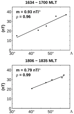
30° 40° 50° 0 10 20 30 40 (nT) ρ = 0.96 m = 0.93 nT/° Λ 1634 − 1700 MLT 30° 40° 50° 0 10 20 30 40 (nT) Λ ρ = 0.99 m = 0.79 nT/° 1806 − 1835 MLT 30° 40° 50° 0 10 20 30 40 (nT) ρ = 0.96 m = 0.93 nT/° Λ 1634 − 1700 MLT 30° 40° 50° 0 10 20 30 40 (nT) Λ ρ = 0.99 m = 0.79 nT/° 1806 − 1835 MLT

Fig. 10. The latitudinal variation of the asymptotic response along

M1 in two narrow MLT strips in the dusk sector. m is the angular coefficient.

indeed, above ∼40◦_{, prenoon values range between 8.6 and} 15.4 nT/(nPa)1/2, while dusk values range between 23.0 and 40.2 nT/(nPa)1/2. Note also that in the entire prenoon sector the geomagnetic response is smaller than in the noon quad-rant at geostationary orbit (∼18.7 nT/(nPa)1/2); conversely, it is explicitly larger in the dusk and night sectors.

The aspects of the latitudinal variation, in the dusk sec-tor, have been better evaluated by focusing attention on two narrow MLT strips (Fig. 10): as a matter of fact we found a strong correlation between the field variation and geo-magnetic latitude, with an average latitudinal gradient that seems to decrease at later MLTs (namely, ∼0.93 nT/◦ at

∼16:45 MLT; ∼0.79 nT/◦at ∼18:15 MLT). It is interesting to remark that approximately the same latitudinal gradient for the H component can be inferred by the experimental re-sults obtained by Petrinec et al. (1996) between 30◦and 60◦, around dusk.

4 Discussion and conclusions

In the present paper we examined several aspects of the mag-netospheric and geomagnetic response to the variable SW conditions observed during a 50-min interval. We focused particular attention on the correspondence between different SW/magnetospheric structures and geomagnetic variations. We carefully examined the aspects of the MLT and

latitu-dinal dependence of the geomagnetic response at low and middle latitudes. We also proposed a new approach to the combined H and D data analysis. This approach allows for a clearer identification of the global geomagnetic response and a better understanding of the results obtained at different sites. On the other hand, this event occurred in the recovery phase after the day the SW almost disappeared: in this sense our results can be useful to examine the aspects of the geo-magnetic response soon after a huge expansion of the Earth’s magnetosphere.

The different aspects of the geomagnetic response (Mat-sushita, 1962; Nishida and Jacobs, 1962) reveal in this case a clear organization in four groups of events. The differences between groups include, in our opinion, several aspects of the more generic “morning/afternoon asymmetry” proposed by previous analysis. Indeed, a visual inspection of the ex-perimental observations reported in the scientific literature suggests that, as for the present case, the transition between structures with different characteristics of the H component typically occurs at later MLTs for higher latitudes (namely, in the early morning hours at ∼30◦–35◦, around noon at ∼55◦– 60◦; Le et al., 1993; Russell and Ginskey, 1995; Tsuno-mura, 1998). Our results also reveal that the different re-sponses at different sites basically reflect a close correspon-dence between the magnetospheric and the ground signals which occur along an axis that progressively rotates from N/S (night events) to an E/W orientation (dawn events). We concluded that a simple two vortex system at these latitudes interprets well all the aspects of the MLT and latitudinal de-pendence, without requesting additional contributions (Rus-sell and Ginskey, 1995): indeed, in agreement with the in-ferred currents, a similar MLT pattern progressively emerges from lower to higher latitudes, with an amplitude modulation much smaller than previously estimated; in addition, a sharp latitudinal dependence is detected in the dusk sector where current lines are perpendicular to geomagnetic meridians.

This event occurred after a prolonged interval of extremely rarefied SW conditions which provided a huge extension of the Earth’s magnetosphere (up to ∼60 Reat ∼19:00 UT, 11 May, Le et al., 2000). The density started to recover after

∼20:00 UT, reaching ∼20 cm−3on 12 May at ∼18:00 UT. Several aspects of the magnetospheric response have been examined in the scientific literature for such peculiar SW conditions. Namely, at geostationary orbit the magneto-spheric field became closely dipolar for ∼16 h (11 May, 12:00 UT–12 May, 04:00 UT, Farrugia et al., 2000); the ground magnetic field disturbances due to the ring current and the magnetopause currents decreased on 11 May to val-ues substantially smaller than quiet times valval-ues (Kp=0+,

Dst between –4 and 10 nT, Jordanova et al., 2001); the pat-tern of the field-aligned currents, at the maximum magne-tospheric expansion, was significantly rotated toward dusk: indeed, while the typical R1/R2 current system was ob-served near dawn, the R0/R1 current system, which is typ-ical of the noon quadrant, was observed near dusk (Othani et al., 2000). Our results allow one to conclude that, on 12 May , ∼15:00 UT, the magnetosphere had already restored

U. Villante and P. Di Giuseppe: Some aspects of the geomagnetic response to solar wind pressure variations 2065 its typical conditions; indeed that, as previously discussed,

most aspects of the geomagnetic response appear consis-tent with a familiar current system. In this sense our con-clusions are consistent with Wind observations that suggest a magnetosonic Mach number of ∼2 in the morning hours and increasing to ∼8–10 in the afternoon hours (Farrugia et al., 2000). Indirectly, interesting results in this sense also come from an analysis of the long period fluctuations de-tected during different time intervals on 12 May. Indeed, the high-latitude observations from IMAGE magnetometer array revealed, between ∼03:00–09:00 UT, prominent spec-tral peaks at ∼0.8 mHz and ∼2.2 mHz (Mathie and Mann, 2000). The latitudinally localized amplitude of these sig-nals and their morphological characteristics were interpreted in terms of field line resonances coupling with discrete cav-ity/waveguide modes of the entire magnetosphere: neverthe-less, the observed frequencies were significantly shifted to lower values than cavity modes frequencies and suggested a still extended magnetosphere supporting unusual cavity modes. Conversely, a few hours later, our analysis of the wave mode following the SI confirms restored magneto-spheric dimensions: indeed, the experimental observations were consistent with a global magnetospheric mode match-ing one of the usual cavity mode frequencies (∼2.8 mHz).

The orientation and latitudinal dependence of the over-shoot field suggests a transient modification of the high-latitude vortex system in the dusk sector. Our results can be considered consistent with theoretical models (Osada, 1992; Araki, 1994) which interpret such overshoot fields (increas-ing with latitude) in terms of the arrival of compressional waves travelling along magnetospheric field lines. On the other hand, overshoot amplitudes are much greater than in other cases. This aspect might be considered consistent with the significant reduction of the ring current in the period of interest (on 12 May, the Dst index progressively increased from 2 to 37 nT between 10:00–18:00 UT, and attained val-ues of 31 nT at 16:00 UT): Russell and Ginskey (1993), in-deed, speculated that a stronger ring current would corre-spond to a higher damping of propagating compressional waves, with a consequent reduction of overshoot amplitudes. Acknowledgements. The key parameters of Wind MFI and SWE, Goes 8 and Goes 10 magnetometers were provided by the NASA Goddard Space Flight Center web site. The ground data are from the CD-ROM of INTERMAGNET “Magnetic Observatory Defini-tive Data”, 1999. Authors are grateful to principal investigators of space and ground experiments. This research activity is supported by MIUR and ASI.

Topical Editor T. Pulkkinen thanks H. L¨uhr and another referee for their help in evaluating this paper.

References

Araki, T. and Nagano, H.: Geomagnetic response to sudden expan-sions of the magnetosphere, J. Geophys. Res., 93, 3983–3988, 1988.

Araki, T.: A physical model of the geomagnetic sudden com-mencement, in Solar Wind Sources of Magnetospheric Ultra-Low-Frequency Waves, Geophys. Monogr. Ser., vol. 81, edited by Engebretson, M. J.,Takahashi, K., and Scoler, M., pp. 183– 200, AGU, Washington, D.C., 1994.

Araki, T., Fujitani, S., Emoto, M., Yumoto, K., Shiokawa, K., Ichi-nose, T., L¨uhr, H., Orr, D., Milling, D. K., Singer, H., Rostoker, G., Tsunomura, S., Yamada, Y., and Liu,,C. F.: Anomalous sud-den commencements on March 24, 1991, J. Geophys. Res., 102, 14 075–14 086, 1997.

Fairfield, D. H., Cairns, I. H., Desch, M. D., Szabo, A., Lazarus, A. J., and Aellig, M. R.: The location of low Mach number bow shocks at Earth, J. Geophys. Res., 106, 25 361–25 376, 2001. Farrugia, C. J., Freeman, M. P., Cowley, S. W. H., Southwood,

D. J., Lockwood, M., and Etemadi, A.: Pressure-driven mag-netopause motions and attendant response on the ground, Planet. Space Sci., 37, 589–607, 1989.

Farrugia, C. J., Singer, H. J., Evans, D., Berdichevsky, D., Scud-der, J. D., Ogilvie, K. W., Fitzenreiter, R. J., and Russell, C. T.: Response of the equatorial and polar magnetosphere to the very tenuous solar wind on 11 May 1999, Geophys. Res. Lett., 27, 3773–3776, 2000.

Francia, P., Lepidi, S., Villante, U., Di Giuseppe, P., and Lazarus, A. J.: Geomagnetic response at low latitude to continuous solar wind pressure variations during northward interplanetary mag-netic field, J. Geophys. Res., 104, 19 923-19 930, 1999. Francia, P., Lepidi, S., Di Giuseppe, P., and Villante, U.:

Geomag-netic sudden impulses at low latitude during northward interplan-etary magnetic field conditions, J. Geophys. Res., 106, 21 231-21 236, 2001.

Francia, P., and Lepidi, S.: Latitudinal dependence of the geo-magnetic response to solar wind pressure variations during the earth’s passage of the 15–16 July 2000 coronal ejecta, Solar cycle and space conference proceedings, Vico Equense (Italy), 24–29 September 2001, ESA SP-477, pp. 431–434, 2002.

Jordanova, V. K., Farrugia, C. J., Fennell, J. F., and Scudder, J. D.: Ground disturbances of the ring, magnetopause, and tail currents on the day the solar wind almost disappeared, J. Geophys. Res., 106, 25 529–25 540, 2001.

Kivelson, M. and Southwood, D. J.: Resonant ULF waves: A new interpretation, Geophys. Res. Lett., 12, 49–52, 1985.

Kivelson, M. and Southwood, D. J.: Coupling of global magneto-spheric MHD eigenmodes to field line resonances, J. Geophys. Res., 91, 4345–4351, 1986.

Kokubun, S.: Characteristics of storm sudden commencement at geostationary orbit, J. Geophys. Res., 88, 10 025–10 033, 1983. Kuwashima, M., and Fukunishi, H.: Local time asymmetries of the

SSC-associated hydromagnetic variations at the geosynchronous altitude, Planet. Space Sci., 33, 711–720, 1985.

Le, G., Russell, C. T., Petrinec, S. M., and Ginskey, M.: Effect of sudden solar wind dynamic pressure changes at subauroral lat-itudes: Change in magnetic field, J. Geophys. Res., 98, 3983– 3990, 1993.

Le, G., Russell, C. T., and Petrinec, S. M.: The magnetosphere on 11 May 1999: the day the solar wind almost disappeared: I. current systems, Geophys. Res. Lett., 27, 1827–1830, 2000.

Mathie, R. A. and Mann, I. R.: Observations of an anomalously low frequency Alfven continuum in an abnormally expanded magne-tosphere, Geophys. Res. Lett., 27, 4017–4020, 2000.

Matsushita, S.: On geomagnetic sudden commencements, sudden impulses, and storm durations, J. Geophys. Res., 67, 3753–3777, 1962.

Nishida, A., and Jacobs, J. A.: World-wide changes in the geomag-netic field, J. Geophys. Res., 67, 525–540, 1962.

Nishida, A.: Geomagnetic Dp2 fluctuations and associated magne-tospheric phenomena, J. Geophys. Res., 73, 1795–1803, 1968. Nishida, A.: Geomagnetic diagnoses of the magnetosphere,

Springer-Verlag, New York, 1978.

Osada, S.: Numerical calculation of geomagnetic sudden com-mencement, Master Thesis, Faculty of Science, Kyoto Univ., March 1992.

Othani, S., Newell, P. T., and Takahashi, K.: Dawn-dusk profile of field-aligned currents on 11 May 1999: A familiar pattern driven by an unusual case, Geophys. Res. Lett., 27, 3777—3780, 2000. Papitashvili, V. O., Clauer, C. R., Christiansen, F., Pilipenko, V. A., Popov, V. A., Rasmussen, O., Suchdeo, V. P., and Watermann, J. F.: Geomagnetic disturbances at high-latitudes during very low solar wind density event, Geophys. Res. Lett., 23, 3785–3788, 2000.

Petrinec, S. M., Yumoto, K., L¨uhr, H., Orr, D., Milling, D., Hayashi, K., Kokubun, S., and Araki, T.: The CME event of 21 February 1994: response of the magnetic field at the Earth’s surface, J. Geomag. Geoelectr., 48, 1341–1379, 1996.

Rostoker, G.: Ground magnetic signatures of ULF and substorm activity during an interval of abnormally weak solar wind on May 11, 1999, Geophys. Res. Lett., 27, 3789–3792, 2000.

Russell, C. T., Ginskey, M., Petrinec, S., and Le, G.: The effect of solar wind dynamic pressure changes on low and mid-latitude magnetic records, Geophys. Res. Lett., 19, 1227–1230, 1992. Russell, C. T., and Ginskey, M.: Sudden impulses at low latitudes:

transient response, Geophys. Res. Lett., 20, 1015–1018, 1993. Russell, C. T., Ginskey, M., and Petrinec, S. M.: Sudden impulses at

low-latitude stations: Steady state response for northward inter-planetary magnetic fields, J. Geophys. Res., 99, 253–261, 1994a. Russell, C. T., Ginskey, M., and Petrinec, S. M.: Sudden impulses at low-latitude stations: steady state response for southward inter-planetary magnetic fields, J. Geophys. Res., 99, 13 403–13 408, 1994b.

Russell, C. T. and Ginskey, M.: Sudden impulses at subauroral lat-itudes: response for northward interplanetary magnetic field, J. Geophys. Res., 100, 23 695-23 702, 1995.

Samson, J. C., Harrold, B. G., Ruohoniemi, J. M., Greenwald, R. A., and M. Walker, A. D.: Field line resonances associated with MHD waveguides in the magnetosphere, Geophys. Res. Lett., 19, 441–444, 1992.

Sastri, J. H., Takeuchi, T., Araki, T., Yumoto, K., Tsunomura, S., Tachihara, H., L¨uhr, H., and Watermann, J.: Preliminary impulse of the geomagnetic storm sudden commencement of November 18, 1993, J. Geophys. Res., 106, 3905–3918, 2001.

Siscoe, G. L.,Formisano, V., and Lazarus, A. J.: Relation between geomagnetic sudden impulses and solar wind pressure changes: An experimental investigation, J. Geophys. Res., 73, 4869–4874, 1968.

Su, S. and Konradi, A.: Magnetic field depression at the Earth’s surface calculated from the relationship between the size of the magnetosphere and the Dst values, J. Geophys. Res., 80, 195– 199, 1975.

Terasawa, T., Kasaba, Y., Tsubouchi, K., Mukai, T., Saito, Y., Frank, L. A., Paterson, W. R., Ackerson, K., Matsumoto, H., Kojima, H., Matsui, H., Larson, D., Lin, R., Phan, T., Stein-berg, J., McComas, D., Skoug, R., Fujimoto, M., Hoshino, M., and Nishida, A.: GEOTAIL observations of anomalously low density plasma in the magnetosheath, Geophys. Res. Lett., 23, 3781–3784, 2000.

Tsunomura, S.: Characteristics of geomagnetic sudden commence-ment observed in middle and low latitudes, Earth Planets and Space, 50, 755–772, 1998.

Villante, U., Francia, P., and Lepidi, S.: Pc5 geomagnetic field fluc-tuations at discrete frequencies at a low latitude station, Ann. Geophysicae, 19, 321–325, 2001.

Villante, U., Francia, P., Vellante, M., and Di Giuseppe, P.: Some aspects of the low latitude geomagnetic response under different solar wind conditions, Space Science Rev., 107, 207–217, 2003. Walker, A. D. M., Ruohoniemi, J. M., Baker, K. B., Greenwald, R. A., and Samson, J. C.: Spatial and temporal behavior of ULF pul-sations observed by the Goose Bay HF radar, J. Geophys. Res., 97, 12 187–12 202, 1992.