Digital filters and applications to seismic detection and discrimination

DIGITAL FILTERS AND APPLICATIONS TO SEISMIC DETECTION AND DISCRIMINATION

by

Jon F. Claerbout

S.B. Massachusetts Institute of Technology (1960)

SUBMITTED IN PARTIAL PULFILLMENT OF THE REQUIREMENTS FOR THE DEGREE OF

MASTER OF SCIENCE at the

MASSACHUSETTS INSTITUTE OF TECHNOLOGY February, 1963

Signature of Author

Certified by

nt

rao elogy & Geophysics Janbary 7, 1963

~' Thsis Supervisor

Accepted bV

Chairman, Departmental Committee on Graduate Students

S I. w ;6 is...6 - a Yi aV K .. - 0 o _ ___. ~~~ ~~____~_~~_~_~ ~~_~~ ___ map , I i I - . I 1- --~~~T-l-T ~'-~3r~- --- ~ -~ -~--"~~-- - ~ -v

ABSTRACT

Title:

Digital Filters and Applications to Seismic

Detection and Discrimination

Author: Joh F. Claerbout

Submitted to the Department of Geology and Geophysics

on January 14, 1963 in partial fulfillment of the

requirements for the degree of Master of Science at

the Massachusetts Institute of Technology

The first part of this thesis is concerned with the

mathematics of filtering in discrete time. Filters are

defined for the purposes of 1) condensing waveforms into

impulsive functions 2) wave shaping 3) noise suppression

4) signal detection according to the criterion of maximum

signal-to-noise output at an instant and 5) the same over

an interval. The behavior of the complex Fourier

trans-forms of some of these filters is considered and connection

is

made

with the theory of orthogonal polynomials.

This

leads to the possibility of a feed back representation of these filters.

In the second part, computational experiments are described in which digital filters are applied to seismic body waves to i) try to determine whether the first arrival is up or down on a seismogram corrupted with microseismic noise, 2) increase signal-to-noise ratio on seismograms

where noise has almost obliterated signal 3) assign polarity to each of two seismic first motion wavelets so they can be termed "same" or "opposite,"

4)

spectral structure of underground nuclear shot seismograms.

Thesis Supervisor: Stephen M. Simpson, Jr.

TABLE OF CONTENTS

INTRODUCTORY EXAMPLES . . . .. . . . . SPIKING FILTERS . * *. . . . . A. Normal Equations. .. . .. . B. Minimum Phase . ...

C. Relation to Orthogonal Polynomials. WAVE SHAPER WITH NOISE ... . .. MATCHED FILTER. ... * ....

MAXIMUM ENERGY SUM FILTER .. . . . . .

. 9 . 9 7 . . 9 9 7 . . . . 12 S. . . .20 * . . • 27

....

27

. .

.

31

0 0

•

*

33

VI FIRST MOTION SPIKING.. .. . . .

VII PREDICTION ERROR EXPERIMENT . * . . . . .

VIII TRAVELLING AUTOSPECTRA OF NUCLEAR SHOT

SEISMOGRAMS...

IX FILTERING FOR SIGNAL TO NOISE IMPROVEMENT

Acknowledgement . . . . . . . . . . Bibliography. ... . . ... . . .. *. 46 *

.

•

55

•

76

.. .

88

. .

89

I

II

IV

V

INTRODUCTION

Although time is a continuous parameter it often happens that observations are made at discrete time inter-vals. Even when continuous observations are made, it is

often desirable to digitize them for computer processing. This is strong reason to do some mathematics in discrete

time. An even stronger reason as we will see is that things which are conceptually quite hard in continuous time have analogues in discrete time which are easier to

understand.

Fortunately,

in discrete time many

general

principles

can be observed with wavelets of very short

time duration.

This

enables us to

consider

some very simple examples

before

launching off into the general theory. These simple examples,

however, will not forshadow

the

way in which

we will connect

the

theory of least

squares filters

with the general theory

of

orthogonal polynomials.

We denote time functions bt with a subscript as the

time parameter. When the time function has finite time durationwe may denote it as b or (bo bI **...bn). Any

time function which has finite energy is called a wavelet. The memory functions of filter* too, are sometimes called wavelets.

I.

Introductory Examples

We introduce the main topics by means of some

examples. One is given in discrete time an input series

(bo,bl) of

length (time duration) two, a filter

(aoa

)

with an impulse response of length two, and the output

resulting from convolution to be

(coc

,c

)

of length

necessarily three. The c is determined from the a and the

b by convolution as is the usual procedure for linear

filters, i.e.

or

1) Spiking

filter

To design a spiking filter one would choose (aopa

)

so that

a

comes

out as closely as possible to a

spike, i.e.

either (1,0,0) or (0,1,0) or (0,0,1).

2)

Wave shaper

To design a wave shaping filter one would choose

(aoal)

so that

c

comes out as closely as possible to some

prescribed waveform (dod ₁d,₂).

3) A matched filter

To design a matched filter one would choose

(aoal)

so that cl comes out as large as possible while making the unit energy constraint ( cCi = ) on the filter. In this problem one doesn't care what co and c2 turn out to be.

4) Maximum energy sum filter

To design a maximum energy sum filter one would choose (ao,al) so that the energy output ( Cf -C C ' ) comes out as large as possible while making the unit energy constraint (

c

A quick sketch of the solutions to these problems is

as

follows:

Since the spiking filter

is a special

case of

the wave shaper

it will be

sufficient

to work out the

solution for the wave shaper. Requiring c' to be as close

as possible to

d

is equivalent to minimizing the squared

distance between them

(C

Setting the partial derivatives with respect to ao and a1

equal to zero we get the simultaneous set for a.

(b

+b

)

a(

+

tb,

b )a,

b d

eb,

d

(b,

b,)

C7

b

)

a+,

b dt + hda

We mention

the

particular

case &d(l,,OO)

called the

zero delay spiking filter.

The solution

of the simultaneous

set is

Recalling

that

subscripts are the time

variable we now

consider the

Pourier transform of

the

solution

The only zero of this complex function is in the upper half of the complex frequency plane, a fact which will be shown true for all zero delay spiking filters. This has considerable importance in feedback systems and in some other connections to be discussed.

The solution to the matched filter problem posed in

3)

above is most easily done by means of

Lagrange muitipliers.

We Wish to maximize c under the constraint

.

Lagrange's method is then to maximize

vnaxL C- o 0 :7- c

(

Setting the derivatives with respect to ao

and a

equal to

C1 )

Thus the filter (aoa 1 ) is simply the signal input

time-reversed and multiplied by a scale factor.

The solution to the maximum energy sum problem 4)

is somewhat like the matched filter. Again one uses Lagranges method and maximizes

C + C - ,\ : a o

by setting derivatives with respect to the components of a equal zero. This results in the equations

bh,

which is the standard eigenvector (i), eigenvalue (N) problem. The two solutions to this problem are

C

and

It is notable that the fourier transform of these functions

have zeros on the real frequency axts. This will also happen with longer filters.

II. Spiking Filters A. Normal Equations

In the first introductory example we considered the

a two term input into a spike function. Now we would like to build an m+l term filter to condense an n+l term input into a spike.

A data wavelet is given by b=(bo,bl,...,bn). We plan to construct a filter a = (aoal,...,am). Filtering is defined in this way: When data b goes into a filter a, an output wavelet c is produced according to the following matrix multiplication.

C

-Y1 _':

_Le

This operation is often called complete transient convolution. This is more loosely written as

ZII

bH

i

(11-2)

-J

Here a small amount of confusion can arise about the limits of the summation because negative subscripts may appear within the summation. What is meant is that one should

consider the terms "off-the-ends" of the wavelets to be zero. With this consideration we might write the limits of the

summation as minus to plus infinity. The artifice of using infinite limits on the sums turns out to avoid some need-lessly cumbersome notation.

Now we introduce another wavelet d which will have the same number of components as c. We call d the desired output of the filter. We saw that c is the actual output. The actual output c was seen to be a function of the input b and the filter a. The problem now is to determine a so

that

c

and

d

are very much

alike.

Specifically

we will choose

a so that the difference vector

1ed

squared (in n+m+l dimensional space).

In other words we

are minimizing

C2 - d)

(11-3)

by varying the components of

a.

Inserting the expression

for

c

in terms

of

a and

b

we get

hl + 11

This function of m+l variables will be minimized if its partial derivative with respect to each of (ao,al,...,am) equals zero. Setting derivatives with respect to af equal zero we get an expression for m+l equations

=1

bD

(7.

b

a

-

;

where one equation is implied for each value of

(

0

-

l

).

These are called normal equations because they say that the error vector, the quantity in brackets, will be normal or perpendicular to the space spanned by the vector set bi. (column vectors in the matrix of equation II-1). We bring the equations into standard form by bringing

the homogeneous part (the part depending on t) to the left side and the inhomogeneous part to the right

'

b

,

b

c

1

b,

9;

(1-6)

t=n J i =e

In matrix form the normal equations become

_b.

b.

--

b,

which can be abbreviate&

BB

a)

Bd~

Jfi

0;l"-be

cb,

..

t b,

\be

bc

and which is identically equal to

The matrix BTB can be written as

I1 roll

*rc-

'I-K

l/

J

h-J

L-C

IF

This r is called the unnormalized transient autocorrelation of b.

dc

(Iz-8)

(II1-9)

7b ,

3;t

We list three special cases of these equations.

1. Zero delay inverse filter

-

This is when

?=

(1,0,0,...,o).

2.

Spiking filter -

This is when the impulse is

chosen any where in d. It has been frequently observed

in practice that putting the impulse near the middle of d

results in an-actual output C which resembles d more

closely than if d had been chosen as in the zero delay case.

3.

Waveshaping

filter

-

This is when

d

is not chosen

to be an impulse at all,

but is chosen to be some arbitrary

wavelet. The filter a then tries to convert the wavelet

b

into the wavelet

d.

It is worth noticing that the homogeneous part of

the normal equations

(II-9)

depends only upon the

autocor-relation of the input b and not on b itself. If the desired

output of the filter is an impulse with no delay

(d

= (1,0,

O,...,0))

then the inhomogeneous part becomes the column

vector

Now in this case we see that the waveform b does not enter the inhomogeneous part either, except for the magnitude of bo . Inspection of the normal equations shows that this

magnitude will not affect the waveform of the filter a except as a scale factor.

Thus the normal equations in this special case (zero delay inverse filter) depend upon the signal waveform, but only through its autocorrelation. Since autocorrelations contain no phase information it would be a curious point as to what the phase spectrum will be of the solution a. We

will study this later and come to the curious conclusion that the phase spectrum is such that as much as possible of the energy in the waveform a is cramped up as close as

possible to

a .

This is called

the property of

minimum

phase delay of the waveform a.

To fix ideas we now give an example of the deter-mination of a zero delay inverse wavelet. Suppose that the signal we are dealing with is the waveform bm(2,l). We want to design a three-term filter $a(ao,al,a 2 ). The

desired output must then _-> be n+m+l = 1+2+1 terms long and

is d = (1,0,0,0). From (II-10) ro = 5, rl = 2, r2 = 0.

The normal equations are

©,

5 1

and the solution is

a

(42,-20,8)/85.

To see how good the

filter is we compare:

actual output c (84,2,4,8)/85

desired output d = (1,0,00)

B.

Minimum Phase

Discussions of minimum phase in the literature are

mostly in terms of continuous time. Here we wish to develop

its properties from the point of view of digital filters which are not so well known. We begin by considering an autocorrelation function of the type of equation (II-11) where

--

(

L

1

-,

,

J

v....

,)

(11-13)

We wonder Vhat functions b might have this autocorrelation. After we have found the class of functions b that have this autocorrelation we can enquire which one has its energy as

close as possible to bo and is, therefore, the minimum phase delay wavelet. One thing which we know to begin with is that more than one wavelet b may have autocorrelation r

(for example; the time reversed waveform, the negative waveform, and the time reverse of the negative waveform).

We begin by spectral considerations. Let F denote Fourier transform. It is commonly known that the energy density spectrum of the wavelet may be expressed in two equal ways:

F2(wQ)

_F

_{F ((c-L}

_(11-14)

Thus the problem is to factor Pr ( , ) into Fb(L) and Pb(t k ) .

Then we can _{simply take the inverse transform of Fb(W)} to get the waveform b. The Fourier transform of T is simply

a-i

(11-15)

and letting z=

e

-

±,+1

2

We notice that the spectrum has been represented as a

poly-nomial in z. The usual procedure in factoring a polynomial

is to find its zeros. Since rk=r.k, we notice that F(Z) is

unchanged if we replace

z

by

z 1

Thus if

Fr(Zo) is

zero

then Fr(/Zo) will also be zero. Thus for every zero z

-1

z

is also a zero. Also since the coefficients of the

polynomial are real the zeros are either real or they occur in conjugate pairs. Thus if zo is a zero then Z0 is a zero.

Most of the zeros will probably occur then in groups of

-four such as

i

\z)

-1

Some of the zeros may occur in groups of two such as

One might wonder about the case

0-t

u

z,0

rd c

where there are two single zeros on the unit circle. It turns out that this can't happen. What we are plotting here is possible locations of zeros of energy density spectra like equation (I-16). When zo iq on the unit

circle 'JJI is real by the relation Z= e . Thus we are talking about the spectrum at some real frequency. A function like the following

which has a single zero at (CQis not an energy density spectrum because it is not positive for all frequencies. More generally, energy density spectra cannot have zeros of odd multiplicity on the unit circle in the .z-plane.

We now know that for every zero Z c-'! - of the energy spectral polynomial that ~ L is another zero. After we factor the spectral polynomial we will be able

to write the spectrum as

Fr7) ^7Z-Ir[()(i 2 *. - (1-1.)

or in terms of W

v-,(

-

er

(II-19)

A (.)l~

Now if we show A( ) e*B( LJ) then we have factored the spectrum Fr(LJ) into the desired conjugate parts

But both are polynomials in

e

be the same function except for a constant multiplicative factor. This can be absorbed from the factor rn

e

This is called factoring the spectrum.

We notice that the factorization could have been done in many ways depending on which of the pair of zeros is put into Fb (t) (the other one then going into Pb(L3)).

Normally, there would be 2n different ways of doing this, the exception being the degenerate case when zeros occur with multiplicity greater than unity. Then there would be fewer than ₂n wavelets with the same energy density. One of these possible factorizations is of parti-cular signifigance. The factoring is done so that all of the zeros which are outsideI of the unit circle are put into Fb(J ) and the opposite member of each pair which is inside the circle then goes into Fb (co ) . In this case the

wavelet must be real because each root is either real or it occurs with its complex conjugate.

Combining all complex roots z with their complex conJugates + )' -) we write for the wavelet's transform

Taking the inverse transform and letting "*" denote con-volution

1 The case with zeros exactly on the unit circle corresponds to a spectrum which is exactly zero for some real LJ . In

any physical case one can usually perturb the spectrum slightly to avoid this difficulty.

(II-19,1)

(II-19,2)

Thus we have a string of convolutions of many

wave-lets each of either 2 or 3 instants duration. Since all

of the roots were chosen outside the unit circle we have

A

>

>

This means that in each of the wavelets the first term is

larger in absolute value than the last. Thus in the

convolution of all terms, the energy will be compacted

toward the beginning. If any one of the zeros had been

chosen instead, from inside the circle, then the energy

would be spread further out on the time axis.

We will now prove that

-7-

(6i)

the summed energy from 0 to any time t for the minimum

phase wavelet is greater or equal to that of anyother

wave-let with the same spectrum.

Consider a two

term wavelet

(b,s) "bigger," "smaller,"

with its zero outside the circle. Convolve it into an

arbitrary wavelet p = (poP ...

,P k). The result is

-1

(b

b,,

by,

spol

.A)

I

If instead we had chosen the reversed wavelet (s,b) with

its zero inside the circle, we would get

A

sNb>pl

(SPC

-4

&w

bj)

Then we consider the partial energy from time = 0 up to time = T and tabulate the difference between iand out to time~ = T and tabulate the diffrence betwen Pin and Pout

ij7(p~-)

TTO

rc

-

i

hu-

(5

r)

±-hp"/

j-

bg)

b

[by,,)

(bpy,

)a

bt.p

Etc

(hkY

(r'

15

)

T--

A~

_(b

_PA)

t-,L4

-0

_ _

= (6)- S-

) p.

-

(s

ok

(b

- ~pl)"

-r Z-

j

- (Sli~?

-

)--_130

Thus we conclude that for any time T the

_{wavelet pout}

with the zero outside the unit circle contains (b2- 2~ more energy in the interval O0 t ~T than the wavelet Pin with the zero inside, The exception is at the last lag when they have both put out the same total energy. It is

not difficult to show that the above statements would still be true if components of vectors were complex and squaring were replaced with multiplying by conjugates.

To prove the minimum phase wavelet delays energy the leasts one imagines that the convolution (11-192) had

been done so that k zeros were outside the circle and n-k were inside, We have just shown that if one of the

zeros from inside were replaced with an outside zero, that the new convolution would have less energy delay. This algument is repeated until all zeros are outuide.

Finally, we show that zero delay spiking wavelets determined by least squares will have all their zeros out-side the unit circle.

We recall the following from previous portions of this thesis:

1) The least-squares spiking wavelet is a wave-let a which when convolved with a given wavelet b tries to give an output equal in the least squares sense to

d = (do,O,0,...,O). Specifically, a is chosen to minimize

' e M h-r

2) We recall that the choice of size of d affects the solution vector a only as a scale factor. Thus do

could always be chosen so that ao a 1. We note that a

scale factor has no effect on a per cent total energy graph,

3) We recall that if a zero of a wavelet is removed from inside the circle and replaced by the conjugate inverse

zero outside, that the modified wavelet has a per cent total energy curve which lies above that of the original wavelet. The per cent total energy curves may touch one another at points except for at time tmO where the curve with fewest zeros inside the circle is definitely ab6ve.

We can view the normal equations a minimizing the energy in a convolve b after time t=O subject to the con-straint that the energy at t=O be equal to (aobo) 2(b) 2 That is, we could view the normal equations as minimizing

the per cent energy after t=O. But this is the same as maximizing the per cent energy at t=0. But if the per-centage energy at t=O is to be maximized for the wavelet a convolve b, then there must be as few as possible zeros inside the circle. This happens if a has none inside and hence is minimum phase.

C. Connection of Least Squares Inverse Filter with Orthogonal Polynomials

Given an energy density function

T (2 )V2

)=

one could take that function and use it as a weighting function to define a set of orthogonal polynomials. We choose the interval of orthogonality to be the unit circle in the z plane which corresponds to the real frequency axis from -4 to + I in the Go plane. Thus we would con-struct a set of polynomials fk

so that

U-10

Tr f * T Y _kh

on the

real

axis.

Expressing

the same thing

with complex

polynomials on the unit circle one gets

h -c

We illustrate the construction of these polynomials in such a way that it will be seen to be equivalent to the

least squares normal equations. Consider the construction

of f2' Let nfr_.1f denote the dot product defined by

equation

(11-20).

The vector f2

is of order two say

C t

-and must satisfy the orthogonality conditions

f(11-22)

Since f2 perpendicular to any linear combination of fo and fl it is perpendicular to any polynomial of order less than 2. Thus the orthogonality relations could be written

(11-23)

This set of orthogonality requirements (II-23) can be written out in full as

[I,

il

c'

+

C1J

c,

[(4-

t-i)

0

[L

J

] coC+

Fzi[7

,

z

c

c

We now examine the coefficients in this simultaneous set. Consider

[Z

Hence the orthogonality relations (II-24) can be written

S

c

r

(11-25)

This is almost exactly the same as the normal equa-tions (11-7) for the least squares inverse filter. The only differences are a scale factor in the inhomogeneous part and "time reversal" of the solution. But this will not affect the waveform c except by a scale factor and time reversal.

Thus we have shown the important result that follow-ing two problems are equivalent:

1) Find polynomials which are orthogonal on the

unit circle with weight )

2) Find least squares zero delay spiking filters of different lengths for the spectrum ~tr(t )

This result is important because it allows us to apply many results in the classic field of orthogonal

polynomials to least squares filter theory.

One application is to use the recurrence relation between successive orthogonal polynomials to generate the filter of length

n+l from the filter of length n. This trick greatly facilitates computing the solution of the normal equations. The relationship for getting

fm+l (Z) from fm(Z) is the recurrence relation (Geronimus 1960)

o(,

oXi,+

1 (11-26)

where the two side conditions used to get

c(Ivl

and second

(

The choice of sign for the square root is immaterial as far as

polynomial orthogonality is concerned. It is customary to choose it

so that _{the first term in the spiking wavelet is positive. The}

recurrence relation can be started off by choosing any value whatever for 4 . _{The result is just a scale factor in the inverse wavelet.} From equation (11-20) it is evident that the recurrence formula can be started off at (A", = () l .

Another readable account is Geronimus (1960). Levinson (1939) also

derived similar, but not identical relations for the filter problem,

although he does not mention any connection with orthogonal polynomialso Levinson's scheme is even more useful than the polynomial recurrence relations because it allows solving the normal equations for arbitrary inhomogeneous part.

Another valuable result of the connection of filter and

poly-nomial theory is the following. All the zeros of all the polynomials generated by the recurrence relation above are known to lie inside the unit circle (Geronimus 1960" _{This means that the time reverse of}

the associated filter is minimum phase. Because of this we can

invert the wavelet, i. e. take the inverse of its spectrum.

S--

b

-_

₁

"

7

Since the polynomial a(z) has no zeros inside the unit circle,

the infinite series b(z) converges at least up to and including the unit circle. This means that the wavelet bk has finite energy and is mini-mum phase. The wavelet a has a spectrum which is in a least squares

sense* equal to l/ ). The spectrum of the infinitely long wavelet b is exactly the inverse of the spectrum of a. Hence we conclude that

the spectrum of b is equal in a least squares sense to

{

( )

phase wavelet of a given autocorrelation function. Futhermore, the

*Least squares in the sense that

fi

computation is quite easy because of the recurrence relation. It is the

most efficient method known to the author who has computed 500 terms

of the minimum phase wavelet in about a minute on an IBM 7090

com-puting machine.

D. A Comment on Autoregressive vs Moving Average Representations A question arises whether it is more efficient to characterize

a stochastic process by the first n terms in its "autoregressive operator"

or by the first n terms of its "moving average operator. " What is meant

by this is the following: Usually filtering is thought of in terms of

convolving filter coefficients b with a data series. This might be called

"moving weighted averages" or more commonly, "moving averages. " This is equivalent to multiplying the Fourier transform of the data

by that of the filter. Substituting z= e it is equivalent to multiply-ing z-transform polynomials which convolves their coefficients.

Filtering could be done in another way called "autoregression. " Instead

of multiplying the data polynomial by b(z) one divides it by the

poly-nomial a(z). This is called 'feedback" filtering for reasons which

should be apparent to anyone who has ever divided polynomials by the

method of synthetic division (see Lanczos 1956).

By "efficiency" we mean the following: suppose we want a filter to representi) and it is easy for us to compute both a and b

quite accurately; in fact, we wish to use many fewer terms than we can

compute. Which characterizes (0) more accurately for small p,

autoregression approximation 1/(ao+a, z+.. +ap z ) ? Whittle (in press) observes that the autoregressive coefficients seem more

efficient and suggests that the reason is that for the series he deals

with -(economic), autoregression is a more realistic physical model.

The author has also observed that the autoregressive coeffiscients

seem more efficient in geophysical time series, but suggests a different

reason. When we digitize continuous functions we usually digitize

at a rate high enough to avoid appreciable frequency fold over. A typical spectrum looks like

\1

The inverse spectrum looks like

Since the inverse spectrum tends to have much more

band-width, its wavelet tends to be shorter. This would indicate that when

these conditions apply a filter using feedback can do a better job for

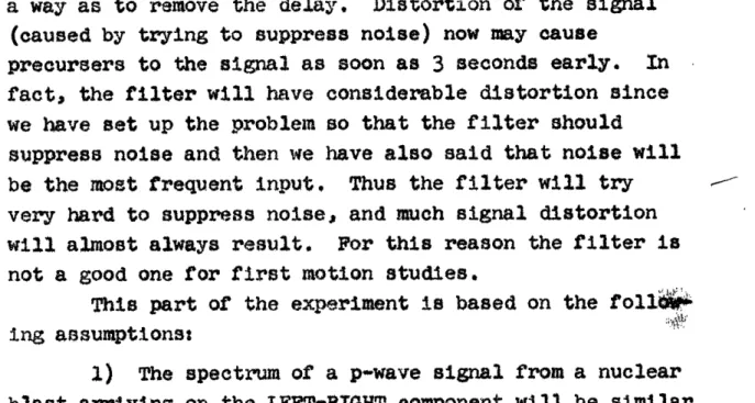
III Generalized Wave Shaper with Noise

A. Derivation of Normal Equations

Here we imagine the following model of a physical

system to apply

Physical System

white light - linear filter b information

Sin _{o m a i n adde}

white light linear filter uk -- noise

constructed filter

desired output

We want to design a filter to operate on the output of the physical

system to give us some preferred output. One set of formulas will

enable us to handle the following problems.

Problem 1. Given the information wavelet bk, the power of the

infor-mation, and the power spectrum of the noise, convert each information

wavelet bk which comes out of the system to some other waveform dk.

For example we may be converting a long drawn out function bk into a

nice short one like a spike or a minimum phase wavelet. Of course, we do not want the filter to respond very much to noise.

spectrum design a filter so that just the information comes out as

uncorrupted as possible. _{The information might be allowed to come out} with some time delay. On the other hand we might want to predict the information before it comes out of the physical system. To see that prediction is a reasonable thing to doconsideri f an extreme case where noise is absent, the linear filter bk "rings" for a long while, and the information white light series consists of impulses widely spaced in time. Of course we cannot predict the onset of a ring, but once a ring starts we can easily predict the rest of it.

Problem 2 was treated by Levinson and Problem 1 was solved by the author in connection with some geophysical problems. They

are very little different. It will be seen that Problem 2 is a special case of Problem 1 so we begin with Problem 1 and specialize the results later.

Let

b

Let

d

Let U be any noise wavelet.

Let _{be a white light series which is convolved with u to give a} statistical model of the noise process.

Let A be a white light series of signal wavelet (b) arrival times.

Let - denote convolution.

The input to the filter is the signal plus noise, i. e., (b-w + u. t ). The actual output will be this convolved with the filter, i. e.

(b

A

The desired output is the wavelet d, occurring every time a signal

wavelet arrives, i. e., G~ . The expected sum squared error is defined as: expected sum squared error = expectation of

(actual output-desired output)"

Since convolution is associative and commutative it is valid

and will be convenient to drop all asterisks in the expansion of the

above square.

By taking the expectation inside, it is seen that the last two terms depend on E( ). We will assume this to be zero. This

means that the signal wavelets arrive at times which are uncorrelated

with the noise wavelets.

We recollect the remaining terms.

(b

A

-

)

7E

From here on the derivation will algebraically resemble that of

the spiking filter. It is convenient to rewrite these convolutions in

subscript summation notation, i. e.

(b

-d)'--J

(j.;

-- ")(b

Oj-

-.

-)

(IC) C

Since we hope to minimize the expected sum squared error we

will take its derivative with respect to each ofithe independent variables

ai and set each one equal to zero. Hence

0 - (III 5)

This can be expressed in more compact form

R~q

R:_

,

b

hk-(III. 6)

having noticed that R and W thus defined are autocorrelation matrices

or Toeplitz matrices. The expression simplifies to:

o=C~lr~

E)

7)a

r

C)

_(isp

CA , - t C,J Cr

I1{

t

-(111- 7)

where

(S

'

J

Utilizing the symmetry of the quantities in the left hand

square brackets we can write:

These equations can easily be rewritten as a matrix equation in the same way as with the spiking filters.

If the desired output dk were just the signal bk

possibly with some lag or some negative lag (prediction)

then the right hand side no longer contains the waveform

bk but only its autocorrelation. This would be the

specialization to Levinson's problem.

We now give some examples writing equation (III-8)

in matrix form.

Example 1

The signal waveform bk

=

(2,1). The signal

arrives with a frequency which gives it an average power

C ,

The noise is white and has unit power. The filter

should have 3 terms. The desired output is a spike after

unit delay, d = (0,1,0,0). The normal equations become

S7 :Z

0

0

C\

,

O

IF

s-

a

I+

Example 2

Like example 1 except the desired output is

the same as the signal input with no delay. The normal

equations are like example I except the right hand side

becomes the column vector (5,2,0)

Example 3

Like example 2 except that the signal should

be predicted by one time unit. The normal equations are

like example 1 except the right hand side because the

column vector (2,0,)T.

IV Matched Filter

Suppose one is given an autocorrelation function of

a noise process and also a signal wavelet. It is desired

to detect the arrival of the signal wavelets in the

pre-sence of the noise. The method to be used is to filter

the incoming mixture of signal and noise and then say that

signals arrive where there are maximums in the output.

How should the filter be designed? If the noise were white and the filter memory wavelet had unit energy, then the power output of the filter with noise as input would be unaffected by the frequency characteristics of the filter. Then the filter need concern itself only with the signal. Thus the introductory example (Section I, no. 4) gives

the whole story when the noise is white. The result is simply that the signal filter coefficients are just the

time reverse of the wavelet and the actual filtering operation then amounts to crosscorrelation of the signal wavelet with the incoming data. If the noise is not white we must do something a bit more complicated.

Using the same notation as the previous section, the power output of the filter with noise input will be the quadratic form

£_)

Vj

magni-fication constant of the filter to be such that this power is unity. This leads to the constraint

For simplicity we choose to make the filter have the same length as the signal wavelet and we choose to have the maximum output come when the wavelet is exactly

in the middle of the filter, i.e., the nth lag of the convolution where both a and b have length n. Thus we maximize

L

(sum

on i)

subject to the constraint equation (IV-1). Using Lagrange multipliers one maximizes

v4' n

-t

-+.I

/\

(

U>

;

L LL

We have differentiated terms exactly like this in previous sections. Letting br represent the time reverse of the

signal wavelet and U represent the noise autocorrelation matrix, we write the result

+

N

(Iv-3)

solving for a we get

A LeTHe

CITr-,

/~

(iv-4)

We can usually ignore 2

X

V)

In practice one may prefer not to invert the matrix in (IV-4) or solve the simultaneous set (IV-3) since there is an easy way around it. One might simply prefilter the data to whiten the noise and then filter with br . The

results would be similar, the difference arising from end effects.

More is known about the matched filter. Suppose one wants to choose a threshold value for the output and

announce "signal" whenever the threshold is exceeded and "no-saignal" when it is not. Then one would like to maximize the probability of guessing correctly. It can be shown that if the noise is gaussian, then the matched filter and pro-per choice of threshold will maximize this probability. V. Maximum Energy Sum Filter

Consider the following physical problem. A trans-ient signal waveform is sent through a dispersive media. The media is such that it may badly disperse the wave without altering its spectral content a great deal. We

know what spectrum to expect of the signal and we know the spectrum of the ambient noise. We would like to design an

VJ

apparatus or procedure to enable us to make a best guess as to when the signal arrives. The matched filter is not

the answer because we do not know the exact signal shape,

only its spectrum. The spiking filter is not appropriate for the same reason. The Wiener-Levinson filter tries to make the output look like the signal input. In this case we don't even know what the input waveform should be, we would Just like to try to decide approximately when it arrives.

A solution to this problem is to design a filter which puts out lots of energy when the signal comes in and minimum power when only noise comes in, Thus our decision would be based on a system like the following:

signal and filter squarer output

noise

-We would search for the time tm when the output was

maximum and then we would say that signal arrived between time tm and time tm-T.

Taking this model then, we seek to maximize

energy output of filter due to signal in interval T

expected

power output due to noise

(V-l)

the same if the noise is white.

Since we are interested in a computer application,

we again specialize ourselves to filters and signals which are discrete in time, and spectra which whose autocorrelations are of finite time duration.

Using the finite autocorrelations of the signal and noise we define two wavelets bit a signal wavelet, and ui ,

a noise wavelet. This can be done be the proceduresdq-cribed earlier. These two wavelets may have different phase spectra than those of our physical problem, but they will have the correct autocorrelation. Thus we begin with

the definitions used earlier:

ai - "ideal" filter coefficients (a_i = 0 if iO or i>M) bi = signal wavelet (bi = 0 if iO or i>N)

ui = noise wavelet (ui = 0 if i<O or i>N)

S = white light series associated with noise process

-has variance 1i.

We use subscript summation notation; the expression

has an implied summation over all values of the repeated index J3 3 goes from minus to plus infinity. Thus the given expression is a vector with free index k and i6 the

complete transient convolution of a and b.

Expression (V-l) for

%

S-

(v-2)

We notice that a quantity like bk-.bk*i is the autocorrelation matrix Bi j of the signal bi and denoting

likewise Ui. j 0 Uji as the autocorrelation matrix of ui,

the expression (V-2) becomes

B/\

o ;

(v-3)

To try to maximize this ratio, we take its partial derivatives with respect to each of the independent variables a) and set them equal to zero.

S-0

nm,

n

(-4)

Multiplying by (Um.naman)

we get

The derivative operations are the same in each term, working only with the first we get

-2,

c,,,

ac

i

o

where S-is the Kronecker delta, Now utilizing the

symmetry of Bi. j and the fact that i and J are dummy

vari-ables, this becomes

tC

K0

Applying this result in equation (V-5), we obtain

This is the generalized eigenvalue problem. Further-more, since B and U are positive definite*, this problem

is known to have M distinct eigenvector solutions for the ai associated with M eigenvalues

A

must be real and positive. Assuming that the eigenvalues are distinct we select for our solution ai that eigenvector which is associated with the maximum eigenvalue. We note

that eigenvectors are determined only to within a scale factor. This corresponds to the physical fact that the

energy power ratio (V-l) will not depend on the amplifica-tion of the filter.

Looking bask to equation (V-2), we see that the numer-ator is the energy in the complete transient convolution

of ai and b_{i , and denominator is likewise for ai} and u_i. The energy in the convolution of two transients is well known to be the integral of the product of their energy density spectra. Therefore, if we were able to find another wavelet ai which had the same amplitude spectrum as ai , we would have another solution to our maximiration

problem.

From the z-transform analysis described in Section II, we know that many finite wavelets may have the same spectra. These different wavelets are obtained (by a

method due

to Wold and also Fe/jer)

_{in the following way:}

1) Compute the autocorrelation of the

given

wavelet.

2) Factor its z-transform.

3)

Its zeros must occur in

pairs, specifically if Zi is a zero, then 1/1i is a zero.

Select _{either one from each pair and form}

(EZ- 1 )(Z-Z 2 )(ZZ 3). This is the z-transborm of a wavelet with the same auto-correlation as the given wavelet. 4) Normally there are

2n possible different wavelets. By the reasoning of the

preceding paragraph, these should all be solutions of our maximization problem.

This is an apparent contradiction to the fact that the eigenvalue problem (V-7) is known to possess a unique *To see that B is positive definite recall that BBA is a quadrati form representing the energy of output when the wavelet b _{goes into the filter a. Clearly this energy is} positive for any real values of a. This means that B is positive definite.

.._1--eigenvector solution ai for the maximum eigenvalue t\ a

The contradiction is resolved if and only if all of the zeros of the z-transform of each solution eigenvector lie on the unit circle. Then the zeros zi equal their inverse

conju-gates i.e.

and the 2n different selections of one from each of the n pairs of zeros all generate the same wavelet.

There is a curious consequence of the fact that the zeros of the z-transform of this filter must be on the unit cirble. It is that the eigenvectors must be either sytmmetric or antisymmetric (for example (2,3,2) or (4,0,-4)

respec-tively). Whether it is symmetric or antisymmetric depends upon whether there are an even or an odd number of zeros at the point Z=I.

This is a simple consequence of the fact that the eigenvectors are real, and any roots of the z-transform which are complex must occur in conjugate pairs. By the main theorem, they must also lie on the unit circle. For

the root

3

and

Hence, the coefficients of the second order and the zero

order terms in z are identical for all

C

symmetric wavelets is symmetric. Hence, the eigenvector would have to be symmetric if all the zeros were complex. However, we also have the possibilitV of zeros at two places on the real axis, -1, and +1. The -1 corresponds

to slymetric wavelet (1,1), and the +1 corresponds to the antisymmetric wavelet (-1,1). Convolution by the first leaves the eigenvector symmetric, but an odd number of con-volutions by the second leave the eigenvector antisymmetric.

Numerical Examle

Let

I) ~

U,;

(tI)(3

i)

6

I

: O

₍

_I?

N

Jo

LI

l0

Xia7y

(

I

- I)

The eigen-values are distinct. The eigenvector

solutions for the maximum and minimum eigen-values are seen to be symmetric, and the remaining eigen-value has an

anti-symmetric eigen-vector. The zeros of the z-transform of

the

eigen-vectors are then computed and plotted:

F

)

/+

=

F4c)

The magnitudes of all the zeros are seen to be equal to I

X41ax

AX ₁

"

;Jt

le

-~

B. Maximum Energy Sum Filter from Spectral Considerations We consider the same problem of determining a filter a_i of finite length in discreet time which is optimum in the sense that it maximizes the ratio:

I

(energy output of filter due to sinal)

I (expected power output due to noise)

This time we solve it in the frequency domain rather than the time domain. Define the filter energy spectrum as A(Wt), the signal energy spectrum as B( w) and the noise power spectrum as G(W). Then the above ratio may be written:

f

-

A(V.B*1)

If the maximum of this ratio is finite then it is

necessary that for perturbations in A( ) we will have I = O. Since A( ) appears in both numerator and denominator it is clear that a multiplicative scale factor in A( )

will be unimportant, in other words we can choose the scale factor as we wish. In fact, we can choose it so that the integral in the demoninator is some constant, i.e.

-1

Then the problem can be restated as maximizing the numerator

S-

subject to the constraint equation (2).

This is a classic problem in the calculus of varia-tions (see for example Hildebrand, Methods of Applied Math, section 2,6). The pro4edure is to maximize the quantity

+ff

-T

-IT

(V.B.4)

subject to no constraint. And then later

X

determined by (2). - is called the Lagrange multiplier. Thus we solve the problem:

-T

(V.B.5)

Since we are dealing with functions in discrete time, the spectra in equation (5) will all be periodic with

period 2 (Nyquists). The spectra are also even functions of (I. Therefore, A, B, and G can always be written as

iqi~

F)EQ')c

r;

C

c-z h L

Fourier cosine series whose coefficients, the Greek letters, can be recognized as the autocorrelation functions of the respective time functions. The limit onl the summation for A(Lu) is finite because the filter ai was chosen to have

finite length and hence so must its autocorrelation. We apply these forms to equation (5).

L+#>

r! s a'2:-oO

_(V.B.7)

hj

The variation is intended to be over the correlation function X of the filter impulse response ai . The 0I(

are not, however, allowed to be varied arbitrarily, they must only be varied in such a way as to keep the energy

density A(U₁W) positive for all L- . In other words an arbitrary selection of the numbers 0(' may not really be an autocorrelation function. Therefore, we will express

the 0(' in terms of the impulse response ai and do the

variation in terms of the ai instead, because any set of

numbers a_i is a valid impulse response. The expressions relating ns; and ai are:

o

a

2

(O0 = a + a + a + . . . . . + a

o 1 = a0al + ala₂ + a2a _{. .. + aN-laN}

o(2 = a0a2 + ala3 + a2a 4 + . . . + aN-2aN

(v.B.8)

N = _ao0aN

Performing the variation merely amounts to writing the Euler equations in terms of the ai , the ai being

completely independent variables. Our integral is of a particularly simple form, therefore, we can obtain greater insight by performing the integration directly. Then we can set the variations (derivatives) with respect to the ai equal to zero.

The integrand is the product of two cosine series., Using the orthonormality of these cosines over the interval + i to -it equation (7) becomes on integration

N _

(VB.9)

C1. C

It is

noteable that the formulas (9)

no longer

contain the

infinite

sum which is in formula

(7).

This

important result will

be referred to later. It means

that only N lags of the

signal

and noise autocorrelations

are needed for the

solution,

N+l being the length of the

impulse response of the filter ai which we are

construct-ing.

We now differentiate the

Ch

aiO

0

if

ai

0

If

i<0

i>N

We now insert this into formula (9) and reorder

terms according to increasing subscripts of aj. This step, although it is complicated amounts to straight-forward symbol manipulation. The final result can be written as the following matrix equation:

q.~

6~c

~

clN

Thus we are led to the same

considerations

(V-7).

One wonders

result as the time domain whether there might

be a useful connection here with the general theory

of

eigenfunctions as there were useful results of connecting

least squares filters with the theory of orthogonal

polynomials.

It is possible and seems likely that some of the

statements

about decision rules,

maximum

likelihood,

etc.

which are made about matched filters in Gaussian noise

could also apply to the maximum energy

sum filter*.

This is a topic which does not appear to have been

inves-tigated,

* This possibility was suggested to the author by both Professor E. M. Hofatetter and Professor T. R. Madden.

SECTION VI First Motion Spiking

A. Object and Motivation

The direction of first mction of the ground at a seismic station has received considerable attention in nuclear detection. The essential idea is that the first motion resulting from an explosive blast should always be upward and away from the epicenter while this would probably not be true for more than half of the time for naturally occurring seismic events. This criterion has been shown to be a reasonable one for the Logan and Blanca test shots for distances less than about 700 km

(Romney, 1959). The primary difficulty _in considering seismograms taken at greater distances was the reduced signal-to-noise ratio further aggravated by the fact that the first motion was in almost all cases smaller than the immediately following oscillations. On some of the seismograms taken at greater distances the first motion appeared to be in the wrong direction despite a fairly strong signal-to-noise ratio. The motivation of the experiment to be discussed is that perhaps the oscilla-tions immediately following the first motion also contain information about the polarity of the first motion, but contain this information in some latent way. This idea is not new, but no effective method has yet been applied to extract this information.

A mathematical technique for extracting this type of information is the spiking filter,

B. Method and Philosophy of the Experiment

First a wavelet, the first motion and several sub-sequent wiggles, is selected from a relatively near-shot, low-noise, seismogram. Then a filter is designed such that with the wavelet as input, it will produce little

or no output before and while the wavelet is entering the filters a large positive spike when the wavelet has fully

entered the filter, and little or no output thereafter. The filter is also designed to have little output when naturally occurring microseisms are its only input. In practically all cases, a filter cannot be designed to do these simultaneous tasks exactly, but the one designed does them in the least-squared-error sense. That the ultimate error will be sufficiently small for practical purposes must be tested computationally.

The filter is then applied to a seismogram with a poorer signal-to-noise ratio which may be at a differ-ent oridiffer-entation to the seismic evdiffer-ent and at a greater distance. If the filtered seismogram consists of low level noise preceding the abrupt arrival of a spike of positive polarity we might then infer that the direction of first motion is the same at the second station as it was at the first, If the impulse had negative polarity we would infer that the second signal had undergone a

180 phase shift with respect to the first signal. If no impulse showed clearly through the background noise, we would infer that this experiment was not successful. To be more precise, in least-squares fitting to a positive impulse we are assigning a polarity to a

clear first arrival wavelet; then we produce a filter which can be applied to wavelets from other seismograms

of the same event which assigns a polarity to each of these.

Finally, we are in a position to examine the possibility that the polarity is the same at all orien-tation ifrom the source. If it is, we infer that the source has rotational symmetry and is probably not of natural origin. If the polarity on the first clear

arrival wavelet is assigned according to the direction of first motion, and if wiggles subsequent to the first

motion really do contain latent information about the first motion, then the hypothesis tested by this experi-ment is very similar to, although not exactly the same

as, the hypothesis that the first motion caused by a

nuclear explosion must be up and away at all source orien-tations, To point out this difference more clearly, con-sider the seismograms mentioned earlier on which the first motions appeared to be in the wrong direction. Possibly the first motion was in the right direction and obscured by the noise, but it might actually have been in the wrong direction. Even if it was, its polarity as deter-mined by the first few wiggles might have been the same as that of other seismograms of the same nuclear event.

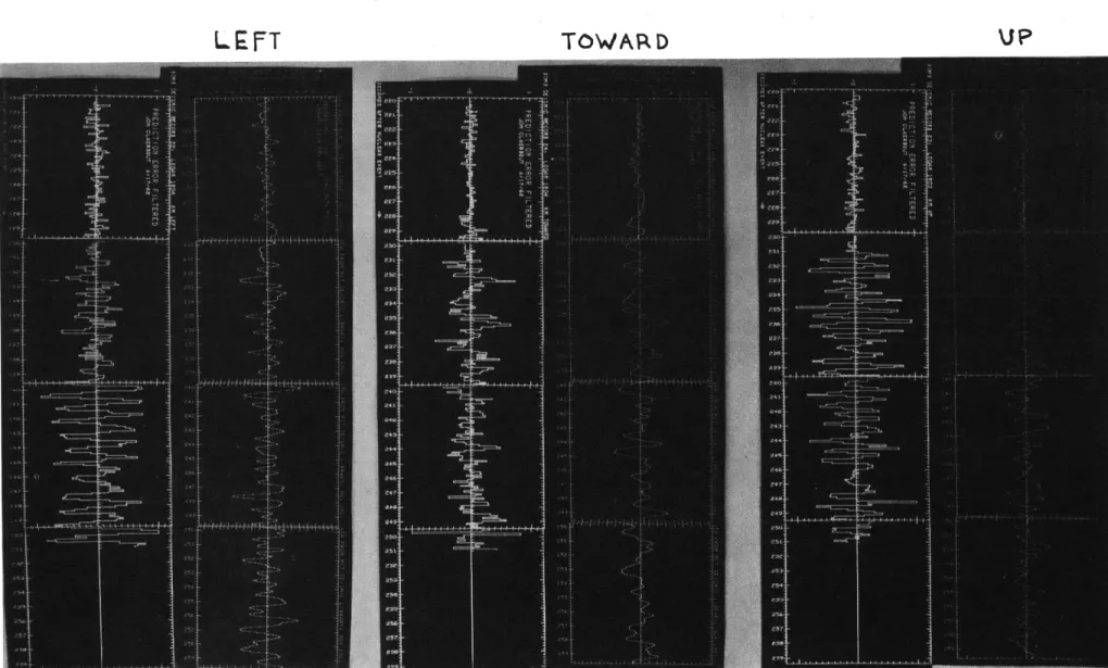
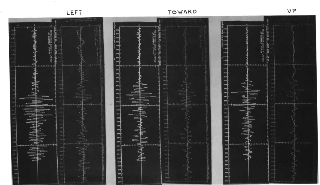
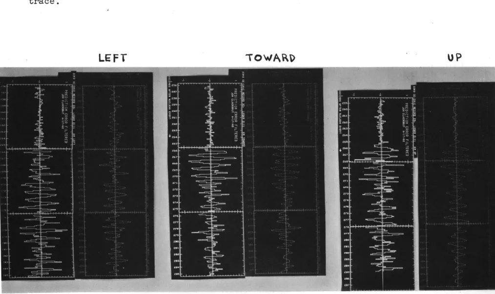
C, Choice of Parameters

Several of the seismic records from the Logan under-ground nuclear explosion:were picked by eye, that is, the first motions were.identified approximately and the first 3.5 to 4.0 seconds of the seismic trace were considered to be the essence of the signal wavelet. The section was then tapered smoothly to zero on each end. The exact way in which this was done is depicted in Figure 1. Only

the shorter of the two wavelets shown (the bottom in each frame) was used. The wavelet length, about 3.75 seconds, was selected because it is long enough to include the

requisite "first few wiggles" but not so long as to make the solution of the simultaneous equations excessively time consuming. A sixty point inverse wavelet which is three seconds in length at our standard digitization rate requires about one minute of IBM 709 time to compute.

The choice of a method of tapering the ends of the wavelet was rather arbitrary. It was motivated by two

considerationst i) The time of the first motion arrival could not be determined exactly, and to be sure that the first motion arrival was included, about 3/4 second of the

seismic trace before the apparent arrival was included in the wavelet. Since it was also felt that the wiggles nearest the first motion probably contain the most infor-mation, wiggles further away were also tapered in amplitude.