HAL Id: insu-01569587
https://hal-insu.archives-ouvertes.fr/insu-01569587
Submitted on 12 Nov 2020HAL is a multi-disciplinary open access archive for the deposit and dissemination of sci-entific research documents, whether they are pub-lished or not. The documents may come from teaching and research institutions in France or abroad, or from public or private research centers.
L’archive ouverte pluridisciplinaire HAL, est destinée au dépôt et à la diffusion de documents scientifiques de niveau recherche, publiés ou non, émanant des établissements d’enseignement et de recherche français ou étrangers, des laboratoires publics ou privés.
Fabry-Perot to measure aerosol and atmospheric
molecular density
Yann Caraty, Alain Hauchecorne, Philippe Keckhut, Jean-François Mariscal,
Eric d’Almeida
To cite this version:
Yann Caraty, Alain Hauchecorne, Philippe Keckhut, Jean-François Mariscal, Eric d’Almeida. High spectral resolution lidar using spherical Fabry-Perot to measure aerosol and atmospheric molecu-lar density. EPJ Web of Conferences, EDP Sciences, 2018, (The 28th International Laser Radar Conference (ILRC 28), Bucharest 2017), 176, art. 01016 (4 p.). �10.1051/epjconf/201817601016�. �insu-01569587�
HIGH SPECTRAL RESOLUTION LIDAR USING SPHERICAL FABRY-PEROT
TO MEASURE AEROSOL AND ATMOSPHERIC MOLECULAR DENSITY
Caraty Yann, Hauchecorne Alain, Keckhut Philippe, Mariscal Jean-François, Dalmeida Eric Affiliation main author: LATMOS, France, [email protected]
Affiliation second, third and fourth author: LATMOS, France ABSTRACT
In theory, the HSRL method should expand the validity range of the atmospheric molecular density and temperature profiles of the Rayleigh LIDAR in the UTLS below 30 km, with an accuracy of 1 K, while suppressing the particle contribution. We tested a Spherical Fabry-Perot which achieves these performances while keeping a big flexibility in optical alignment. However, this device has some limitations (thermal drift and a possible partial depolarisation of the backscattered signal). 1 INTRODUCTION
Temperature is a main parameter for the radiative, dynamic and chemical processes of the atmosphere. The measure of the vertical profile of this variable is therefore a major challenge in the meteorological and climatic context.
Analysis of the temperature parameter requires a global and complete spatial coverage, a good vertical resolution and a temporal continuity of the measurements. Various techniques for analysing the vertical profile of atmospheric temperature exist. The LIDAR (Light Detection and Ranging) allows the measure of this profile in accordance with the previous requirements through the Rayleigh technique [1] [2].
This technique involves vertically emitting a short light pulse via a laser towards the atmosphere at a wavelength corresponding to the atmospheric constituents scattering. The method involves then collecting the photons of the pulsed laser beam which are backscattered by the atmospheric particles by means of a telescope pointing to the zenith in the emission direction.
In the upper stratosphere (above 30 km), the backscattered signal comes only from Rayleigh or molecular scattering by air molecules (there are no aerosols). The number of photons recorded is directly proportional to the atmospheric density. This one can be used to trace back to the atmospheric temperature vertical profile (via the ideal gas law and the assumption of an atmosphere in hydrostatic equilibirum with a constant air mass [3]).
In the upper troposphere and the lower stratosphere (the UTLS below 30 km), aerosols contaminate the backscattered signal which now comes from two scatterings: molecular scattering (by air molecules) and Mie or particle scattering (by aerosols). The Rayleigh LIDAR method hence becomes inapplicable.
The technique developed involves using spectral filtering to eliminate the particle scattering contribution within the LIDAR signal below 30 km. This is made possible by the Doppler broadening of the Rayleigh line shape, the linewidth of the particle scattering being equivalent to the linewidth of the laser [4]. Thus, the High Spectral Resolution Lidar (HSRL) method aims to expand the validity range of the atmospheric molecular density and temperature profiles of the Rayleigh LIDAR in the UTLS [5]. The subject of this article is therefore to introduce an atmospheric molecular density and temperature measurement technique using an innovative HSRL method developed around a Spherical Fabry-Perot (SFP) [6].
In a first part, we describe the HSRL technique with this SFP and discuss its implementation in the optical box of the Rayleigh LIDAR in operation at the Observatory of Haute-Provence (OHP). Then, we present and analyse the initial results. Finally, we conclude with the performances and limitations of this method and discuss its potential for improvements. 2 METHODOLOGY
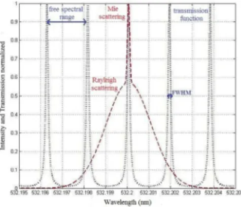
2.1 The principle of the HSRL technique The HSRL method is based on using the line shapes of the light beam backscattered by the atmospheric constituents. In the UTLS, a backscattered line shape (by molecular and particle scatterings) is represented by the superposition of two curves focusing on the same wavelength [7]: a Voigt profile similar at a Gaussian curve (molecular contribution) whose broadening depends on the temperature and pressure values superimposed with a thin central peak (aerosols contribution) whose broadening is conditioned by the characteristics of the laser [4] (Fig. 1).
The principle of the HSRL method is to use a filtering device (as the SFP) whose transmission function makes it possible to discriminate between the Rayleigh and particle contributions within the backscattered signal in the UTLS. The objective is to measure the atmospheric temperature profile from the analysis of the molecular portion of the backscattered line shape. The transmission function selects a spectral line finer than the Rayleigh line shape but broader than the particle line shape (Fig. 1).
Figure 1:
Simulation of the backscattered line shape at 532.2 nm by molecular and particle scatterings at T ≈ 220 K (red). Simulation of the SFP transmission function (blue). According to the specifications from the company Spectra Physics (Nd:YAG laser pulsed at λ0 = 532.2 nm and single-mode through injection) and taking into account an average temperature of T ≈ 220 K within the UTLS, the SFP should make it possible to isolate a ΔλMie<0.168 pm linewidth from a background width of ΔλRayleigh≈2.12±0.10 pm (Fig. 1). The objective is to retain the aerosols contribution by eliminating almost all of the molecular component. If the characteristics of the filtering system are know, it is then possible to isolate the Rayleigh and particle signals through calculation. Finally, this estimate of the molecular scattering unpolluted makes it possible to infer the temperature profile through the Rayleigh LIDAR method as in the upper stratosphere [3] [5]. 2.2 Description and general properties of the SFP The principle of the SFP was developed by Pierre Connes in 1958 to specifically study hyperfine structures and line shapes as small as 10-3 cm-1. This is a unit-magnification afocal system consisting of two identical concave spherical blades which are each centred on top of one another.These blades are restricted by circular diaphragms of diameter D. They are both connected by two flat blades produced from a material having a zero expansion coefficient. So, the system is stiffened bymolecular adhesion (Fig. 2.a).
In this study, the SFP is in a hermetic metal enclosure equipped with an adjustable screw so that the volume and pressure can be mechanically modified, and in turn, the refractive index of internal air n (Fig. 2.b). So, we can spectrally adjust this filtering device on the λ0 laser wavelength by changing the pressure between the blades.
Figure 2.a and 2.b:
Photograph of the SFP in its metallic box (a). Photograph of the external appearance of the SFP (b). However, the peculiarity of the SFP concerns the light paths in the device and at its output (Fig. 3).
Figure 3:
Diagram of the SFP with the internal light paths (projection on a main section plane). This specificity results in the angular independence of the δ optical path difference (δ = 4.n.e with the thickness e) and the transmission of the SFP unlike the case of the Plane Fabry-Perot (PFP). This filtering device is characterised by its thickness e which can be equated to the curvature radius. However, the thickness of this filtering system is fixed and cannot be modified unlike for the PFP. The spherical interferometer also has characteristics similar to those of a double thickness PFP. It has
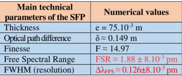
the same transparency, contrast and finesse F. The R0 theoretical resolving power, the δ0resolution limit and the free spectral range also are identical [6]. It is thus possible to define the SFP transmission function thanks to the PFP theory with a double reflection and the angular independence (Fig. 3). Here, we developed a SFP of thickness e=75.10-3m equivalent to a single thickness PFP with a finesse of F ≈ 30 and a power reflection coefficient of R ≈ 0.900. The characteristics of this SFP are summarized in table 1.
Table 1:Summary of the main technical parameters of the SFP.
Main technical
parameters of the SFP Numerical values
Thickness e = 75.10-3 m
Optical path difference δ ≈ 0.149 m
Finesse F ≈ 14.97
Free Spectral Range FSR ≈1.88 ± 8.10-3 pm
FWHM (resolution) ΔλFPS ≈ 0.126±8.10-3 pm Finally, with ΔλFPS=FWHM≈0.126±8.10-3 pm, this spherical interferometer is able to select a spectral line finer than the Rayleigh line shape (ΔλRayleigh≈2.12±0.10pm) and as broad as the particle line shape (ΔλMie<0.168 pm). Its transmission function thus has the ability to differentiate the molecular and aerosols contributions within the backscattered signal (Fig. 1 and table 1). So, the SFP is a filter transmitting only the energy emitted by the laser source within its bandwidth. 2.3 Characterisation of the optical set-up The filtering system is implemented in the optical analysis box of the Rayleigh LIDAR in operation at the OHP whose the optical set-up is investigated in Fig. 4 and [3].
Figure 4:
Diagram of the optical set-up of the LIDAR station at the OHP. The Nd:YAG laser vertically emits a short monochromatic light pulse towards the atmosphere at λ0 = 532.2 nm. The laser beam first passes through the emission system which reduces its divergence through an afocal optical device. The backscattered photons are then collected by the reception telescope pointing to
the zenith in the direction of the emission (Fig. 4).
An optical fiber placed at the main mirror's focal point ensures the transmission of the signal to the optical box (Fig. 4). Inside this, the light beam begins by passing through an interference filter that eliminates atmospheric noise (Fig. 4). Finally, the signal is dissociated into two channels (with the SFP on the second channel) by a beam splitter 50/50 and sensed by two photomultipliers (PMs) R7400U-20 in "photon counting" mode (Fig. 4).
3 INITIAL RESULTS
We present the results for the night of 22nd to 23rd July 2015 between 21:35 UT and 22:35 UT with the presence of low-lying cirrus (Fig. 5). The profiles are represented between 682 m (altitude of the station) and 40 km with a vertical resolution of Δz = 150 m. The optical set-up analyses two output signals (Fig. 4): the S1(z) signal corresponding to the channel without SFP (channel 1) and the S2(z) signal corresponding to the channel with the SFP (channel 2). S1(z) is the total of the laser photons backscattered by air molecules (Nm(z)) and by almost all the aerosols (Na(z)). S2(z) is proportional to the sum of the photons backscattered by air molecules (Tm(z).Nm(z)) and by the aerosols (Ta.Na(z)) transmitted by the SFP. These signals show that the aerosols distribution is generally diffuse within the UTLS with the exception of areas with relatively dense cloud cover between 7 km and 9 km and between 10 km and 11 km where we detect high particle concentrations which result in an increase in the number of the backscattered photons (intensity peaks of the S1(z) and S2(z) profiles). The combination of S1(z) and S2(z) signals leads to the Nm(z) molecular and Na(z) particle density vertical profiles (equations (1) and (2)):
Nmz = Q1 Q2.S2z - Ta.S1z Tmz - Ta (1) Naz = S1z - Nmz (2) Analysis of Na(z) confirms that the aerosols contribution to the backscattered signal in the UTLS is to be taken into account only at the level of cloud covers. The acquisition range of the Nm(z) profile spans the interval [2.5 ; 20] km (Fig. 5). The number of the photons backscattered by air molecules decreases exponentially as altitude increases (Fig. 5). This decrease is coherent with a diminishing molecular concentration as altitude increases and a particle distribution which is generally diffuse within the UTLS. However, the main interest of this profile lies in the flattening of intensity peaks in ranges [7 ; 9] km and [10 ; 11] km (Fig. 5).
The partial ([7 ; 9] km) or total ([10 ; 11] km) suppression of these peaks means that we have succeeded in considerably limiting the aerosols contribution to the backscattered signal in the UTLS.
Figure 5:
Representation of the Nm(z) experimental molecular density profile in the UTLS for the night of 22nd to 23rd July 2015 between 21:35 UT and 22:35 UT at the OHP. Ultimately, the HSRL method with the SFP improves the capabilities of the Rayleigh LIDAR by extending its validity range to the UTLS between 2.5 km and 20 km altitude. However, the reliability of this technique decreases when the particle concentration is too high (here between 7 km and 9 km altitude). The aerosols contribution is then only minimised and there remain a particle residue of about 15 % which cannot be corrected (Fig. 5).
Two phenomena may restrict these performances. This could be a problem of partial depolarisation of the backscattered signal associated with the operating mode of the optical box. One solution would be to retain only one polarisation in the optical box through a polarising beamsplitter cube at its input. The spectral adjustment of the laser source with the SFP has also to be considered. Indeed, we note a Δλdéc ≈ 0.10 ± 8.10-3 pm spectral shift of the device relative to λ0 at the end of the experimental phase. This, because of a thermal drift of the laser and/or the SFP. The solution is to control their internal temperature through an automatic monitoring system. 4 CONCLUSIONS
Finally, with a resolution of ΔλFPS≈0.126±8.10-3 pm, the SFP is able to select a ΔλMie<0.168 pm linewidth from a background width of ΔλRayleigh≈2.12±0.10 pm. This filtering device therefore seems well adapted to separate the molecular and aerosols contributions within the backscattered laser signal in the UTLS. Thus, the HSRL method with this SFP improves the capabilities of the Rayleigh LIDAR at the OHP by extending its validity range to the UTLS between 2.5 km and 20 km altitude.
The SFP offers many advantages relative to the cumbersome parameterisation of the PFP (thickness > 8 cm and diameter > a few centimeters) with regard to achieving the resolution levels necessary within the framework of these studies of hyperfine structures from 10-3 cm-1. Despite its performances, these capabilities decrease when the particle concentration is too high. The problems stem in particular from the possible partial depolarisation of the backscattered signal and the probably thermal drift of the laser source and/or the SFP. Improvements in this filtering technique (integration of a polarising beamsplitter cube and an automated temperature control device) will soon form the basis for the design of a new instrument of higher precision. ACKNOWLEDGEMENTS
This work has drawn heavily on research conducted by Pierre Connes in 1958. Virginia Ciardini contributed to this study during her masters degree in 2005. REFERENCES
[1] Hauchecorne A., Chanin M. L., 1980: Density and temperature profiles obtained by Lidar between 35 and 70 km, Geophys. Res. Lett., 7, 565-568. [2] Chanin M. L., Hauchecorne A., 1984:
Lidar studies of temperature and density using scattering, Map Handb., 13, 87-89. [3] Keckhut P., Hauchecorne A., Chanin M. L., 1993: A Critical Review of the Database Acquired for the Long-Term Surveillance of the Middle Atmosphere by the French Rayleigh Lidars, J. Atm. Ocean. Tech., 10, 850-867. [4] Fiocco G., Benedetti-Michelangeli G.,
Maischberger K., Madonna E., 1971: Measurement of Temperature and Aerosol to Molecule Ratio in the Troposphere by Optical Radar, Nature Physical Science, 299, 78-79. [5] Hauchecorne A., Chanin M. L., Keckhut P., Nedeljkovic D., 1992: Lidar monitoring of the temperature in the middle and lower atmosphere, Appl. Phys., B55, 29-34.
[6] Connes P., 1958: L'étalon de Fabry-Pérot Sphérique, Le journal de physique et le radium, 19, 262-269.
[7] Fiocco G., De Wolf J. B., 1968: Frequency Spectrum of Laser Echoes from Atmospheric Constituents and Determination of the Aerosol Content of Air, J. Atmos. Sci., 25, 488-496.