DT-REFinD: Diffusion Tensor Registration
With Exact Finite-Strain Differential
The MIT Faculty has made this article openly available.
Please share
how this access benefits you. Your story matters.
Citation
Yeo, B.T.T. et al. “DT-REFinD: Diffusion Tensor Registration With
Exact Finite-Strain Differential.” Medical Imaging, IEEE Transactions
on 28.12 (2009): 1914-1928. © 2010 Institute of Electrical and
Electronics Engineers.
As Published
http://dx.doi.org/10.1109/TMI.2009.2025654
Publisher
Institute of Electrical and Electronics Engineers
Version
Final published version
Citable link
http://hdl.handle.net/1721.1/58791
Terms of Use
Article is made available in accordance with the publisher's
policy and may be subject to US copyright law. Please refer to the
publisher's site for terms of use.
DT-REFinD: Diffusion Tensor Registration
With Exact Finite-Strain Differential
B.T. Thomas Yeo*, Tom Vercauteren, Pierre Fillard, Jean-Marc Peyrat, Xavier Pennec, Polina Golland,
Nicholas Ayache, and Olivier Clatz
Abstract—In this paper, we propose the DT-REFinD algorithm for the diffeomorphic nonlinear registration of diffusion tensor images. Unlike scalar images, deforming tensor images requires choosing both a reorientation strategy and an interpolation scheme. Current diffusion tensor registration algorithms that use full tensor information face difficulties in computing the differential of the tensor reorientation strategy and consequently, these methods often approximate the gradient of the objective function. In the case of the finite-strain (FS) reorientation strategy, we borrow results from the pose estimation literature in computer vision to derive an analytical gradient of the registration objective function. By utilizing the closed-form gradient and the velocity field representation of one parameter subgroups of diffeomor-phisms, the resulting registration algorithm is diffeomorphic and fast. We contrast the algorithm with a traditional FS alternative that ignores the reorientation in the gradient computation. We show that the exact gradient leads to significantly better reg-istration at the cost of computation time. Independently of the choice of Euclidean or Log-Euclidean interpolation and sum of squared differences dissimilarity measure, the exact gradient achieves better alignment over an entire spectrum of deformation penalties. Alignment quality is assessed with a battery of metrics including tensor overlap, fractional anisotropy, inverse consistency and closeness to synthetic warps. The improvements persist even when a different reorientation scheme, preservation of principal directions, is used to apply the final deformations.
Index Terms—Diffeomorphisms, diffusion tensor imaging, fi-nite-strain (FS), fifi-nite-strain differential, preservation of principal directions, registration, tensor reorientation.
Manuscript received April 20, 2009; revised June 09, 2009. First published June 23, 2009; current version published November 25, 2009. This work was supported by the INRIA Associated Teams Program Compu-Tumor (http://www-sop.inria.fr/asclepios/projects/boston/), by the NAMIC under Grant NIH NIBIB NAMIC U54-EB005149, and by the NAC under Grant NIH NCRR NAC P41-RR13218). The work of T. Yeo was supported by the Agency for Science, Technology, and Research, Singapore. Asterisk indicates
corresponding author.
*B.T. T. Yeo is with the Department of Electrical Engineering and Computer Science, Massachusetts Institute of Technology, Cambridge, MA 02139 USA (e-mail: ythomas@csail.mit.edu).
P. Golland is with the Department of Electrical Engineering and Computer Science, Massachusetts Institute of Technology, Cambridge, MA 02139 USA (e-mail: polina@csail.mit.edu).
T. Vercauteren is with the Mauna Kea Technologies, 75010 Paris, France (e-mail: tom.vercauteren@maunakeatech.com).
P. Fillard, J.-M. Peyrat, X. Pennec, N. Ayache, and O. Clatz are with the Asclepios Group, INRIA, 06902 Sophia Antipolis, France (e-mail: pierre.fillard@sophia.inria.fr; jean-marc.peyrat@sophia.inria.fr; xavier.pennec@sophia.inria.fr; nicholas.ayache@sophia.inria.fr; olivier. clatz@sophia.inria.fr).
Color versions of one or more of the figures in this paper are available online at http://ieeexplore.ieee.org.
Digital Object Identifier 10.1109/TMI.2009.2025654
I. INTRODUCTION
D
IFFUSION tensor imaging (DTI) noninvasively measures the diffusion of water in in vivo biological tissues [8]. The diffusion is anisotropic in tissues such as cerebral white matter. DTI is therefore a powerful imaging modality for studying white matter structures in the brain. The rate and anisotropy of diffu-sion at each voxel of a diffudiffu-sion tensor image is summarized by an order 2 symmetric positive definite tensor, i.e., a posi-tive definite 3 3 matrix. This is in contrast to scalar values in traditional magnetic resonance images. The eigenvectors of the tensor correspond to the three principal directions of diffu-sion while the eigenvalues measure the rate of diffudiffu-sion in these directions.To study the variability or similarity of white matter struc-tures across a population or to track white matter changes of a single subject through time, registration is necessary to estab-lish correspondences across different diffusion tensor (DT) im-ages. Registration can be simplistically thought of as warping one image to match another. For scalar images, such a warp can be defined by a deformation field and an interpolation scheme. For DT images however, one also needs to define a tensor reori-entation scheme. Reorireori-entation of tensors is necessary to warp a tensor image consistently with the anatomy [3]. There are two commonly used reorientation strategies: the finite-strain (FS) re-orientation and the preservation of principal directions (PPD) reorientation. In this paper, we derive an exact differential of FS reorientation strategy and show that incorporating the exact differential into the registration algorithm leads to significantly better registration than the common practice of ignoring the re-orientation when computing the gradient [3]. Their empirical performance is similar [23], [34], [49].
Many DTI registration algorithms have been proposed [2], [15], [24], [28], [31], [36], [49], [50]. Because the reorientation strategies greatly complicate the computation of the gradient of the registration objective function [49], many of these registra-tion techniques use scalar values or features that are invariant to image transformations. This includes the use of fractional anisotropy [31] and fibers extracted through tractography [50]. Leemans et al. [28] use mutual information to affinely align the diffusion weighted images from which the DT images are estimated. Nonlinear fluid registration of DT images based on information theoretic measures has since been introduced [16], [39].
Instead of using deformation invariant features, Alexander and Gee [2] perform elastic registration of tensor images by re-orienting the tensors after each iteration using PPD reorienta-tion. The reorientation is not taken into account when computing
the gradient of the objective function. Cao et al. [15] propose a diffeomorphic registration of tensor images using PPD reorien-tation. The diffeomorphism is parameterized by a nonstationary velocity field under the large deformation diffeomorphic metric mapping (LDDMM) framework [11]. An exact gradient of the PPD reorientation is computed by a clever analytical reformu-lation of the PPD reorientation strategy. In this paper, we com-plement the work in [15] by computing the exact gradient of the FS reorientation.
For a general transformation, such as defined by B-splines or nonparametric free form displacement field, the FS reorienta-tion [3] is defined through the rotareorienta-tion component of the defor-mation field. This rotation is estimated by the polar decomposi-tion of the Jacobian of the deformadecomposi-tion field using principles of continuum mechanics. The rotation produced by the polar de-composition of the Jacobian is the closest orthogonal operator to the Jacobian under any unitary invariant norm [26]. However, the polar decomposition requires computing the square root of a positive definite matrix, which replaces the eigenvalues of the original matrix with their square roots. The dependence of the rotation matrix on the Jacobian of deformation is therefore com-plex and the gradient of any objective function that involves re-orientation is hard to compute.
Zhang et al. [48], [49] propose and demonstrate a piecewise local affine registration algorithm to register tensor images using FS reorientation. The tensor image is divided into uniform re-gions and the optimal affine transformation is then estimated for each such region. The rotation component of the deforma-tion need not be estimated as a separate step. Instead, since rota-tion is already explicitly optimized in the affine registrarota-tion, the gradient due to FS reorientation can be easily computed. These piecewise affine transformations are fused together to generate a smooth warp field. The algorithm is iterated in a multiscale fashion with smaller uniform regions. Unfortunately, it is un-clear how much of the optimality is lost in fusing these locally optimal piecewise affine transformations.
In this paper, we borrow results from the pose estimation lit-erature in computer vision [20] to compute the analytical differ-ential of the rotation matrix with respect to the Jacobian of the displacement field. We propose a diffeomorphic DTI registra-tion algorithm DT-REFinD, which extends the recently intro-duced diffeomorphic Demons registration of scalar images [42] to registration of tensor images. The availability of the exact an-alytical gradient allows us to utilize the Gauss–Newton method for optimization. Implemented within the Insight Toolkit (ITK) framework, registration of a pair of 128 128 60 diffusion tensor volumes takes 15 min on a Xeon 3.2 GHz single pro-cessor machine. This is comparable to the nonlinear registration of scalar images whose runtime might range from a couple of minutes to hours. DT-REFinD has been incorporated into the freely available MedINRIA software.1
The diffeomorphic Demons registration algorithm [42] is an extension of the popular Demons algorithm [37]. It guar-antees that the transformation is diffeomorphic. The space of transformations is parameterized by a composition of
deforma-1MedINRIA can be downloaded at
http://www-sop.inria.fr/asclepios/soft-ware/MedINRIA.
tions, each of which is parametrized by a stationary velocity field. Such a representation is similar to that used by the large deformation diffeomorphic metric mapping (LDDMM) frame-work [11], [38]. However, unlike LDDMM, the diffeomorphic Demons algorithm does not seek a geodesic of the Lie group of diffeomorphism. At each iteration, the diffeomorphic Demons algorithm seeks the best diffeomorphism to be composed with the current transformation. Restricting each deformation up-date to belong to a one parameter subgroup of diffeomorphism results in a faster algorithm than the typical algorithm based on the LDDMM framework or algorithms that parameterize the entire diffeomorphic transformation by a stationary velocity field [7], [25].
In addition to DT-REFinD, we also propose a simpler and faster algorithm that ignores the reorientation during the gra-dient computation. Instead, reorientation is performed after each iteration. This faster algorithm is therefore a diffeomorphic variant of the method proposed by Alexander and Gee [2] with Gauss–Newton optimization. We compare the two algorithms and show that using the exact gradient results in significantly better registration at the cost of computation time.
While many methods for interpolating and comparing tensor images exist [27], [32], we use Euclidean interpolation and sum-of-squares difference (EUC-SSD) [2], [3], [49], as well as Log-Euclidean interpolation and sum-of-squares difference (LOG-SSD) [6], [21]. Regardless of the choice of interpo-lation and dissimilarity metric, we find the exact gradient achieves better alignment over an entire range of deforma-tion regularizadeforma-tion. Alignment quality is assessed with a set of seventeen different metrics including tensor overlap, frac-tional anisotropy and inverse consistency of the warps. We also find that the exact gradient method recovers synthetically generated warps with higher accuracy. Finally, we show that the improvements persist even when PPD is used to apply the final deformations.
We emphasize that there is no theoretical guarantee that using the true gradient will lead to a better solution. After all, the reg-istration problem is nonconvex and any solution we find is a local optimum. In practice however, the experiments show that taking reorientation into account does significantly improve the registration results. We believe that the reorientation provides an additional constraint. The registration algorithm cannot arbi-trarily pull in a faraway region for matching because this induces the reorientation of tensors in other regions (cf. the famous “C” example in large deformation fluid registration [18]). This ad-ditional constraint acts as a further regularization, leading to a better solution.
This paper extends a previously presented conference article [47] and contains detailed derivations, experiments and discus-sions left out in the conference version. The paper is organized as follows. The Section II describes the computation of the FS differential. We then present an overview of the diffeomorphic Demons algorithm in Section III and discuss certain conventions and numerical limitations of representing diffeomorphic trans-formations. We extend the diffeomorphic Demons to tensor im-ages in Section IV using the exact FS differential. We also pro-pose a simpler and faster algorithm that ignores the reorientation during the gradient computation. In Section V, we compare the
two algorithms on a set of 10 DT brain images. Further discus-sion is provided in Section VI.
To summarize, our contributions are as follows. 1) We derive the exact FS differential.
2) We incorporate the FS differential into a fast diffeomorphic DT image registration algorithm. We emphasize that the FS differential is useful, even if one were to use a different registration scheme with a different model of deformation or dissimilarity metric.
3) We demonstrate that the use of the exact gradient leads to better registration. In particular, we show that using the exact gradient leads to better tensor alignment over an en-tire range of deformation, regardless of whether we use LOG-SSD or EUC-SSD in the objective function. We also show that the exact gradient recovers synthetically gener-ated deformation fields significantly better than when using an approximate gradient that ignores reorientation. 4) Our implementation allows for Euclidean interpolation and
EUC-SSD metric, as well as Log-Euclidean interpolation and LOG-SSD metric.
II. FINITE-STRAINDIFFERENTIAL
Deforming a tensor image by a transformation involves tensor interpolation followed by tensor reorientation [3]. To compute a deformed tensor at a voxel , one first interpolates the tensor to get the interpolated tensor . Interpolation schemes include Euclidean interpolation [3], Log-Euclidean interpolation [6], affine-invariant framework [10], [22], [29], [30], [32], Geodesic–Loxodromes [27], or other methods. In this work, we focus on Euclidean and Log-Euclidean interpola-tion since they are commonly used and computainterpola-tionally simple. The FS differential we compute in this section characterizes tensor reorientation. The following discussion is therefore independent of the interpolation strategy.
Suppose the transformation maps a point to the point . Let be the displacement field associated with the transformation . Then
(1) Similarly, we denote . Note that even for parametric representation of transformations, such as splines, one can al-ways derive the equivalent displacement field representation.
According to the FS tensor reorientation strategy [3] for non-linear deformation, one first computes the rotation component of the deformation at the th voxel
(2) where is the Jacobian of the spatial transformation at the voxel
(3)
where are the components of the displacement field in the , and directions. is called a polar decomposition of the matrix and is therefore a function of the displace-ment field in the neighborhood of . Under the identity trans-formation, i.e., zero displacements, and . Because of the matrix inverse in (2), to maintain numerical sta-bility of the computations, the invertista-bility of the deformation (corresponding to ) is important.
The interpolated tensor is then reoriented, resulting in the final tensor
(4) For registration based on the FS strategy, it is therefore neces-sary to compute the differential of rotation with respect to the transformation . Using chain rule, this reduces to computing the differential of rotation with respect to the Jacobian . Let be the infinitesimal change in the Jacobian . Then, as shown in Appendix A, the infinitesimal change in the rotation matrix
is computed as follows:
(5) where , denotes the 3-D vector cross product, denotes the th column of and is the operator defined as
(6) This skew-symmetric operator is actually the matrix represen-tation of cross-product, so that for two vectors and ,
. It is introduced to simplify the notation in the already com-plicated (5).
The detailed derivation, based on the pose estimation solution [20] is presented in Appendix A. Let be th component of . Equation (5) tells us the variation of the rotation in terms of the components of the Jacobian . In particular, is computed by setting the matrix in (5) to 0, except for which is set to 1.
III. BACKGROUND ONDIFFEOMORPHICREGISTRATION
In this section, we briefly review the diffeomorphic exten-sion [42] of Thirion’s Demons algorithm [37]. We also discuss numerical issues related to representing diffeomorphism by ve-locity fields and optimization methods we use in this paper.
A. Diffeomorphic Demons for Scalar Images
We consider the modified Demons objective function [14] for registering a moving scalar image to a fixed scalar image
(7) where is the dense spatial transformation to be optimized, is an auxiliary spatial transformation, denotes composition and denotes the -norm of a vector (or vector field, depending on the context). We can think of the fixed image and warped moving image as 1-D vectors of length voxels. is a diagonal matrix that defines the variability observed at a
particular voxel. and are parameters of the cost function. The instantiation of these parameters are further discussed in Section V-B.
This formulation enables a fast and simple optimization that alternately minimizes the first two terms and the last two terms of (7). Typically, , encouraging and to be close and , encouraging to be smooth. The regularization can also be modified to handle a fluid model. We note that and can together be inter-preted probabilistically as a hierarchical prior on the deforma-tion [46].
For the classical Demons algorithm and its variants, the objective function is optimized over the complete space of nonparametric spatial transformations [14], [35], [37], [43], typically represented as displacement fields. Unfortunately, the resulting deformation might not be diffeomorphic. Instead, Vercauteren et al. [42] optimize over compositions of diffeo-morphic deformations, each of which is parametrized by a stationary velocity field. At each iteration, the diffeomorphic Demons algorithm seeks the best diffeomorphism parame-terized by the stationary velocity , to be composed with the current transformation.
In this case, the velocity field is an element of the Lie al-gebra and is the diffeomorphism associated with . The operator is the group exponential relating the Lie Group to its associated Lie algebra . More formally, let be the solution at time of the following stationary or-dinary differential equation (ODE):
(8) We define
(9) An image is therefore a deformed version of image obtained by transforming the coordinate system of by : a point in the deformed coordinate system corre-sponds to a point in the old coordinate system.
The above formulation of the Demons objective function fa-cilitates a fast iterative two-step optimization. We summarize the diffeomorphic Demons algorithm [42] in Algorithm 1 (see algorithm at the top of the page). Steps 2(ii) to 2(iv) essentially optimize the last two terms of (7). We refer the reader to [13], [14] for a detailed discussion of using convolution kernels to achieve elastic and fluid regularization. We also note that the above formulation is quite general, and in fact the diffeomorphic
Demons algorithm can be extended to non-Euclidean domains, such as the sphere [46].
B. Numerical Details in Velocity Field Representations
While and are technically defined on the entire continuous image domain, in practice, and are represented by vector fields on a discrete grid of image points, such as voxels [37], [42] or control points [7], [11]. From the theories of ODEs, we know that the integral curves (or trajectories) of a velocity field exist and are unique if is Lipschitz continuous in and continuous in [12]. Uniqueness means that the trajectories do not cross, implying that the deformation is invertible. Further-more, we know from the theories of ODEs that a contin-uous velocity field produces a continuous deformation field . Therefore, a sufficiently smooth velocity field re-sults in a diffeomorphic transformation.
Since the velocity field is stationary in the case of the one parameter subgroup of diffeomorphism [5], is clearly contin-uous (and in fact ) in . A smooth interpolation of is con-tinuous in the spatial domain and is Lipschitz concon-tinuous if we consider a compact domain, which holds since we only consider images that are closed and bounded.
To compute the final deformation of an image, we have to estimate at least at the set of image grid points. For ex-ample, we can compute by numerically integrating the smoothly interpolated velocity field with Euler integration. In this case, the estimate becomes arbitrarily close to the true as the number of integration time steps increases. With a sufficiently large number of integration steps, we expect the estimate to be invertible and the resulting transformation to be diffeomorphic.
The parameterization of diffeomorphism by stationary ve-locity field is made popular by the use of the fast “scaling and squaring” approach to computing [5]. Instead of Euler integration, the “scaling and squaring” method works by mul-tiple composition of displacement fields
.. .
(10) While this method is correct in the continuous case, in the discrete case, composition of the displacement fields requires
interpolation of displacement fields, introducing errors in the process. In particular, suppose and are the true trajectories found by performing an accurate Euler integration up to time and respectively. Then, there does not exist a trivial interpolation scheme that guarantees . In practice however, it is widely reported that “scaling and squaring” tends to preserve invert-ibility even with rather large deformation [5], [7], [42]. In this work, we employ trilinear interpolation because it is fast. We find that in practice, the transformation is indeed diffeomorphic. Technically speaking, since we use linear interpolation for the displacement field, the transformation is only homeomorphic rather than diffeomorphic. However, we will follow the con-vention of [5], [7], [42] which call the resulting homeomorphic transformations diffeomorphisms.
C. Gauss–Newton Nonlinear Least-Squares Optimization
We now focus on the optimization of step 2(i) of the diffeo-morphic Demons algorithm. We choose
, where
. We “subtract” the identity transformation from the resulting deformation field so that the identity transformation carries no penalty. The objective function in step 2(i) can then be written in a nonlinear least-squares form
(11) (12) (13) where we define and
. Using Taylor series expansion around , we can write (13) as
(14) To interpret (14) for 3-D images with voxels, let be a vector of components:
.
Then is a block diagonal matrix, whose th block corresponds to a 1 3 matrix
(15)
(16) (17) (18) (19) where is the transformation of voxel and is the identity transformation when the velocity . In (17), we utilize the fact that the differential of the exponential map at is the identity. is the
spatial derivative of the image intensity at voxel of the warped moving image .
Similarly, we can show that where is a identity matrix. The Gauss–Newton optimiza-tion method ignores the term within the norm in (14), leading to the classical linear least-squares problem. In partic-ular, (14) can then be rewritten as
(20) (21) which is a linear least-squares problem. Independently of the size of the matrices, it is easy to solve the resulting linear system since the equations for each voxel can be decoupled from all other voxels. With the help of the Sherman-Morrison matrix inversion lemma, no matrix inversion is even needed to invert the resulting small system of linear equations at each voxel [42].
We note that the original Demons algorithm [37] replaced by . This is justified by the fact that at the op-timum, the gradient of the warped moving image should be al-most equal to the gradient of the fixed image.
IV. DT-REFIND: TENSORIMAGEREGISTRATION
A. Diffeomorphic Demons for Vector Images
Before incorporating the FS differential for tensor regis-tration, let us extend the diffeomorphic Demons algorithm to vector images. In addition to helping us explain our complete algorithm, the derivation will also be useful for computing up-date steps when ignoring tensor reorientation in Section IV-D. We define a vector image to be an image with a vector of inten-sities at each voxel. We can treat a vector image like a scalar image in the sense that each vector component is independent of the other components. Deformation of a vector image works just like a scalar image, by treating each component of the vector separately.
It is fairly straightforward to re-derive the results from the previous section for vector images. Let be the dimension of the intensity vector at each voxel. For convenience, we define
to be the intensity vector of the th voxel, , and to be the vector of all image intensities . Then the diffeomorphic Demons algorithm from the previous section applies exactly to vector images except that in (20), is now a sparse block diagonal matrix, where each block is . In particular, the th block of contains spatial derivatives of at voxel
..
. ... ... (22) The resulting least-squares linear system is slightly harder to solve than before. However, for each voxel , we only have to solve a 3 3 linear system for the velocity vector update
. The solution of the system is also more stable as there are more constraints.
B. DT-REFinD: Diffusion Tensor Registration With Exact FS Differential
We will now extend the Demons algorithm to DT images. A DT image is different from a vector image because of the additional structure present in a tensor. In particular, the space of symmetric positive definite matrices (tensors) is not a vector space. When deforming a DT image, reorientation is also nec-essary. We extend the diffeomorphic Demons registration of vector images to tensor images.
In this work, we use the modified Demons objective function (7) and the FS reorientation strategy in our registration. The ob-jective function in step 2(i) of the Demons algorithm, shown in (11) for scalars, becomes
(23) (24) (25) Here, is the Euclidean sum of squares difference (EUC-SSD) between the tensor images. In particular, can be seen as a vector by “rasterizing” the 3 3 order 2 tensor at each voxel into a column vector. should be interpreted as the interpolated tensor image. In practice, since the tensors are symmetric, we can work with vectors to represent tensors and increase the weights of the entries of corresponding to the nondiagonal entries of the tensors by . Each interpolated tensor is then reoriented using the rotation matrix of each voxel and “rasterized” into a column vector. Note that is implicitly dependent on the transformation . The term computes the SSD between each tensor of the fixed image and the corresponding reoriented and interpolated tensor in the warped moving image, by treating each tensor as a vector and adding the SSD for all voxels.
Equation (23) can also be interpreted as the LOG-SSD be-tween tensors if and are the Log-Euclidean transforms of the original tensor images, obtained by converting each tensor
in the original image to a log-tensor . Note that is simply a symmetric matrix [6]. is then the in-terpolated log-tensor image. is the in-terpolated and reoriented log-tensor image, since
(26)
for any rotation matrix . Therefore, tensor reorientation followed by Log-Euclidean transformation is the same as Log-Euclidean transformation followed by reorientation. This is convenient since we can perform a one time Log-Euclidean transformation of the tensor images to log-tensor images before registration and convert the final warped log-tensor images to tensor images at the end of the registration.
In this case, is a sparse matrix. One can interpret as blocks of 9 3 matrices. In particular, the th block is equal to , where we remind the readers that and , are also voxel indices. Using the chain rule, the product rule and the fact that the differential of the exponential map at is the identity, we get
(27) (28) (29)
(30) where is the identity transformation when the velocity . Recall that is a function of the Jacobian of displacement field at the voxel and that (3) gives an analytical ex-pression of . In practice, is defined numerically using finite central difference as shown in (31) at the bottom of the page where are the neighbors of voxel in the , and directions, respectively. Therefore denotes the -coordinate of after transformation and denotes the -coordinate of after transformation . , and are the voxel spac-ings in the , and directions respectively. Using the differ-ential of (5) and the expression of (31), we can compute using the chain rule. Appendix B provides the detailed derivation. This definition of implies
(32)
and for neighbor of voxel , we get
(33) Note that the first and second terms in the above expression are transpose of each other. Therefore, for , the th block of is zeros if voxels and are not neighbors.
As before, . In summary, we have computed the full gradient of our objective function
(34) where is a constant diagonal matrix, while is a sparse matrix.
C. Gauss–Newton Nonlinear Least-Squares Optimization
From the previous sections, we can now write
(35) (36) The resulting least-squares problem is harder to solve than be-fore, since the linear systems of equations cannot be separated into voxel-specific set of equations. However, the sparsity of the matrix makes the problem tractable. In practice, we solve the linear systems of equations using Gmm++, a free generic C++ template library for solving linear sparse systems.2At the finest
resolution, solving the sparse linear system requires about 60 s. This is the bottleneck of the algorithm. However, due to the fast convergence of Gauss–Newton method, we typically only need to solve the linear systems 10 times per multiresolution level. The resulting registration takes about 15 min on a Xeon 3.2 GHz single processor machine.
The efficiency of the Demons algorithm for scalar images comes from separating the optimization into two phases: op-timization of the dissimilarity measure and opop-timization of the regularization term. This avoids the need to solve a nonseparable system of linear equations when considering the two phases to-gether. Because of the reorientation in tensor registration, we have to solve a sparse system of linear equations anyway. In this case, we could have incorporated the optimization of the regularization term together with the optimization of the dissim-ilarity measure without much loss of efficiency. In this work, we keep the two phases separate to allow for fair comparison with the case of ignoring the reorientation of tensors in the gradient computation (see Section IV-D) by using almost the same im-plementation. Any improvement must then clearly come from the use of the true gradient and not from using a one-phase op-timization scheme versus a two-phase opop-timization scheme.
2http://home.gna.org/getfem/gmm_intro
D. Classical Alternative: Ignoring the Reorientation of Tensors
Previous work [2] performs tensor registration by not in-cluding the reorientation in the gradient computation, but reorienting the tensors after each iteration using the current estimated displacement field. To evaluate the utility of the true gradient, we modify our algorithm to ignore the reorientation part of the objective function in the gradient computation. In particular, we can simplify the Gauss–Newton optimiza-tion in the previous secoptimiza-tion by setting and , effectively ignoring the effects of the displacement field of a voxel on the reorientation of its neighbors. Note that is slightly different from before because we directly use the gradient of the warped and reoriented image. In each iteration, we treat the tensor like a vector, except when deforming the moving image. The resulting least-squares problem degenerates to that in Section IV-A. The algorithm is thus much faster since we only need to invert a 3 3 matrix per voxel at each iteration. Registration only takes a few minutes on a Xeon 3.2 GHz single processor machine.
V. EXPERIMENTS
We now compare the DT-REFinD algorithm that uses the exact FS differential with the classical alternative that uses an approximate gradient and a basic Demons algorithm that uses the fixed image gradient.
A. Data and Preprocessing
We use 10 DT images acquired on a Siemens 1.5T scanner using an EPI sequence, consisting of healthy volunteers with the following acquisition parameters: echo time ; 25 diffusion gradients, image dimensions ; image resolution . These images are kindly contributed by Dr. Ducreux, Bicêtre Hospital, Paris, France.
We first use morphological operations to extract a foreground mask from the diffusion weighted (DW) images of each of the 10 DT images. This involves an automatic thresholding of any single DW image, except the baseline, so that the skull and the eyes do not interfere in the mask calculation. The threshold is chosen so that the mask contains the entire brain. This in-evitably contains some outliers in the background. Then, a se-quence of erosions with a ball of radius 1 voxel is performed to remove outliers (3 to 4 iterations are sufficient), which re-sults in a set of connected components ensured to lie within the brain. Finally, we use conditional reconstruction to create the final mask. This involves dilating the connected components while intersecting the result with the initial mask, and repeating this process until convergence. Doing so allows the connected components to grows within the brain while ensuring the back-ground outliers are canceled. If holes are still present in the mask, a hole filling algorithm can be applied (a simple morpho-logical closing is generally sufficient).
B. Implementation Details
We perform pairwise registration of DT images via a standard multiresolution optimization, by smoothing and downsampling the data for initial registration and using the resulting registra-tion from a coarser resoluregistra-tion to initialize the registraregistra-tion of a finer resolution. We find that 10 iterations per multiresolution level were sufficient for convergence. When computing the SSD objective function, only voxels corresponding to the fixed image foreground are included.
There are three main parameters in the algorithm: the diag-onal variability matrix , and the tradeoff parameters and . could be, in principle, estimated from a set of diffusion tensor images via coregistration. Since we deal with pairwise registration, we set to be a constant diagonal matrix. Con-sequently, because the local optimum is determined by the rel-ative weighting of , and , we simply set to be the identity matrix. determines the step-size taken at each iter-ation, which affects the stability of the registration algorithm [42]. Therefore, we empirically set so that the update at each iteration is about 2 voxels. The relative values of and de-termine the width of the kernel used to smooth the deformation field. Once is determined, the value of determines the warp smoothness.
As previously shown [14], it does not make sense to com-pare two registration algorithms with a fixed tradeoff between the dissimilarity measure and regularization, especially when the two algorithms use different dissimilarity measures and/or regularizations. Furthermore, one needs to be careful with the tradeoff selection for optimal performance in a given applica-tion [44].
In this work, we compare the algorithms over a broad range of kernel sizes. We note that larger kernel sizes lead to more smoothing and thus smoother warps. Because kernel sizes are not comparable across the different algorithms we consider, we use harmonic energy as a more direct measure of warp smooth-ness. We define the harmonic energy to be the average over all voxels of the squared Frobenius norm of the Jacobian of the dis-placement field. Note that the Jacobian of the disdis-placement field corresponds to the Jacobian of the transformation defined in (3) without the identity. Therefore lower harmonic energy corre-sponds to smoother deformation.
C. Evaluation Metrics
To assess the alignment quality of two registered DT images, we use a variety of tensor metrics [2], [9], [21]. Let be a dif-fusion tensor. We let , , be its eigenvalues in descending order with corresponding eigenvectors , , . We denote the average eigenvalues. Similarly, let denote another diffusion tensor with corresponding eigenvalues , and eigenvectors . The following measures are averaged over the foreground voxels of the fixed image. This in turn al-lows us to average results across different registration trials by normalizing for brain sizes.
1) Euclidean Mean Squared Errors (EUC-MSE): squared Frobenius norm of .
2) Log Euclidean Mean Squared Errors (LOG-MSE): squared Frobenius norm of .
3) 1—Overlap: . Note that the EUC-MSE and LOG-MSE correspond to the SSD and LOG-SSD dissimilarity metrics we employ during registra-tion. In additional to these tensor metrics, we also consider the following scalar measures [1], [9]. The dissimilarity between two tensors is defined to be the sum of squared differences between these scalar measures, averaged over the foreground voxels.
1)
.
2) LFA (Logarithmic Anisotropy): FA computed for . 3) ADC (Apparent Diffusion Coefficient): . 4) VOL (Volume): .
5) CL (Linear Anisotropic Diffusion): . 6) CP (Planar Ansiotropic Diffusion): . 7) CS (Spherical Anisotropic Diffusion): . 8) RA (Relative Anisotropy): . 9) VR (Volume Ratio): . 10) DISP (Dispersion): . 11) . 12) . 13) .
A question then arises over whether these scalar measures should be computed after deforming the moving image or computed on the unwarped moving image and then interpolated with the deformation field. The latter is attractive because the result is independent of the tensor reorientation and interpola-tion strategies. On the other hand, since registrainterpola-tion is almost never an end-goal—the deformed tensor images are presum-ably used for other tasks, one could argue that it is important to measure the quality of the deformed tensors. Therefore, in this work, we consider both strategies. Finally, we define the average distance between two deformation fields and to be
(37) where is the number of foreground voxels. We compute the average difference in the deformation fields obtained by the dif-ferent methods to evaluate how difdif-ferent the deformation fields are. We find that the average difference in the deformation fields between the exact gradient method and the approximate gra-dient method ranges from 2 mm at low harmonic energy to 5 mm at high harmonic energy (cf. image resolution
). The average difference in the deformation fields between the fixed image gradient method and the other two methods ranges from 3 mm at low harmonic energy to 8 mm at high harmonic energy.
The average distance can also be used to measure inverse con-sistency. Without the availability of ground truth deformation, inverse consistency [17] can be used as an indirect assessment of deformation quality. In particular, given a deformation from subject to subject and from subject to subject , inverse
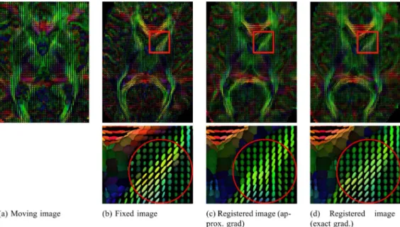
Fig. 1. Qualitative comparison between the exact FS gradient and the approximated gradient for registering a pair of subjects using the Log-Euclidean framework and the same parameters in the registration. (a) Moving image. (b) Fixed image. (c) Registration using the approximated moving image gradient. (d) Registration using the exact FS gradient. Volumes were slightly cropped for better display. Exact gradient achieves better alignment of fiber tracts with a smoother displacement field. Tensors in the anterior limb of the internal capsule, highlighted in (b) and (d) are coherently oriented in a north-east direction. However, in (c), the directions of the tensors are more scattered. Furthermore, the volume of the tensors in (c) is swollen relative to (b) and (d). Numerically, the exact FS gradient has lower SSD with a smoother deformation field (not shown).
consistency is defined to be the average distance between the displacement field associated with the composed warp
and a zero displacement field.
D. Qualitative Evaluation
Fig. 1 shows an example registration of two subjects from our data set. Visually, DT-REFinD results in better tract alignment, such as the anterior limb of the internal capsule highlighted in the figure. See figure caption for more discussion. In this partic-ular example, DT-REFinD also achieves a better Log-Euclidean mean-square-error (LOG-MSE) and smoother deformation as measured by the harmonic energy.
E. Quantitative Evaluation I
To quantitatively compare the performance of the exact FS gradient, the approximate gradient and the fixed image gradient, we consider pairwise registration of the 10 DT images. Since our registration is not symmetric between the fixed and moving images, there are 90 possible pairwise registration experiments. We randomly select 20 pairs of images for pairwise registra-tion. By swapping the roles of the fixed and moving images, we obtain 40 pairs of image registration. From our experiments, we find that the statistics we compute appear to converge after about 30 pairwise registrations, hence 40 pairwise registrations are sufficient for our purpose.
Even though we are considering algorithms with the same dissimilarity measure and regularization (and effectively the same implementation) but different optimization schemes, we find that for a fixed-size smoothing kernel, using the exact FS differential tends to converge to a solution of lower harmonic energy, i.e., a smoother displacement field. Smaller harmonic energy implies a smoother deformation, providing evidence that the reorientation acts as an additional constraint for the
registration problem. To properly compare the algorithms, we consider smoothing kernels of sizes from 0.5 to 2.0 in increments of 0.1. In particular, we perform the following experiment.
For each pair of subjects and for each kernel size
i) Run the diffeomorphic Demons registration algorithm using Euclidean interpolation and EUC-SSD using:
(a) Exact FS gradient (DT-REFinD).
(b) Approximate gradient by ignoring reorientation. (c) Fixed image gradient. This is the gradient proposed
in Thirion’s original Demons algorithm [37]. ii) Repeat (i) using Log-Euclidean interpolation and
LOG-SSD.
iii) Use the estimated deformation fields to compute the tensor and scalar measures discussed in Section V-C using FS reorientation or PPD reorientation.
iv) Compute the inverse consistency of the deformations from subject to subject and from subject to subject . For a given smoothing kernel and registration strategy, registering different pairs of images leads to a set of error metric values corresponding to different harmonic energies. To average the error metric values across different pairs of images and to compare registration results among different strategies, for each registration, we linearly interpolate the dissimilarity metric (EUC-MSE, LOG-MSE, and so on) over a fixed set of harmonic energies sampled between 0.03 to 0.3. This allows us to average the error metric across different pairs of images and compare different strategies at a given harmonic energy.
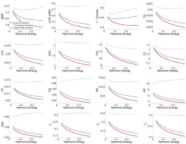
1) Tensor Alignment: Fig. 2 shows the error metrics
(av-eraged over 40 pairwise registrations) with respect to the har-monic energies when using the dissimilarity metric EUC-SSD, euclidean interpolation and FS reorientation for registration. The final deformations were applied using FS reorientation.
Fig. 2. Comparison of exact FS gradient, approximate gradient and fixed image gradient over an entire spectrum of harmonic energy (x-axis) using EUC-SSD, Euclidean interpolation and FS reorientation for registration. The final deformations are applied using FS reorientation. We find that the exact FS gradient method achieves the best performance.
Fig. 3 shows the corresponding plot when applying the final warps using PPD reorientation. In both cases, we find that at all harmonic energy levels, the exact FS gradient method achieves the lowest errors. The approximate gradient method outperforms the fixed image gradient method.
As mentioned earlier, the scalar measures, such as FA, can be computed after deforming the moving tensor image or computed on the unwarped moving image and then deformed. Figs. 2 and 3 show results based on the former strategy. We obtain similar results using the latter strategy, but omit them here for brevity.
The amount of improvement increases as the harmonic ener-gies increase. In our experiments, a harmonic energy of 0.3 cor-responds to severe distortion (pushing the limits of the numer-ical stability of scaling and squaring), while a harmonic energy of 0.03 corresponds to very smooth warps. In previous work, we showed in the context of image segmentation that extreme dis-tortion causes overfitting, while extremely smooth warps might result in insufficient fitting [44]. Only a concrete application can inform us of the optimal amount of distortion and is the sub-ject of future studies. For now, we assume a “safe” range for assessing the algorithm’s behavior to be between harmonic en-ergies 0.1 and 0.2. From the values in Figs. 2 and 3, we conclude that the exact FS gradient provides an improvement of between 5% to 10% over the approximate gradient in this “safe” range of harmonic energies.
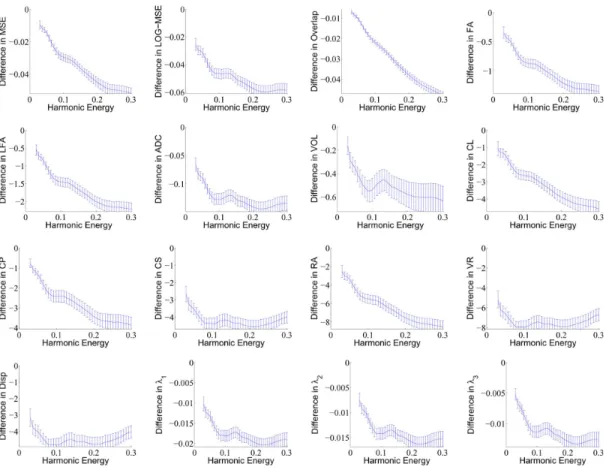
To better appreciate the improvements, Fig. 4 shows the dif-ference in errors by subtracting the error metric values of the approximate gradient method from the error metric values of the exact gradient method when using the dissimilarity metric EUC-SSD, Euclidean interpolation and FS reorientation for reg-istration. The final deformations were applied using FS reorien-tation. The error bars indicate that the exact gradient method is statistically significantly better than the approximate gradient method over the entire range of harmonic energies and all the error metrics ( for almost entire range of harmonic en-ergies). We emphasize that the improvements persist even when we evaluate a different dissimilarity measure or use a different reorientation strategy from those used during registration.
Similarly, we find that the exact FS gradient method achieves the lowest errors when using LOG-SSD similarity metric and Log-Euclidean interpolation for registration, regardless of whether FS or PPD reorientation was used to apply the final deformation. We omit the results here in the interest of space.
2) Inverse Consistency: Fig. 5 shows the inverse consistency
errors (averaged over 20 sets of forward and backward pair-wise registrations) with respect to the harmonic energies. Once again, we find that all harmonic energy levels, the exact FS gra-dient method achieves the lowest errors, regardless of whether EUC-SSD and Euclidean interpolation or LOG-SSD and Log-Euclidean interpolation were used. Similarly, the approximate gradient method outperforms the fixed image gradient method.
Fig. 3. Comparison of exact FS gradient, approximate gradient and fixed image gradient over an entire spectrum of harmonic energy (x-axis) using EUC-SSD, Euclidean interpolation and FS reorientation for registration. The final deformations are applied using PPD reorientation. We find that the exact FS gradient method achieves the best performance.
F. Quantitative Evaluation II
We perform a second set of experiments to evaluate the algo-rithm’s ability to recover randomly generated synthetic warps. Given a DT image, we first generate a set of random warps by sampling a random velocity at each voxel location from an inde-pendent and identically distributed (I.I.D.) Gaussian. The fore-ground mask is then used to remove the velocity field from the background voxels. The resulting velocity field is smoothed spa-tially with a Gaussian filter. We compute the resulting displace-ment field by “scaling and squaring.” This displacedisplace-ment field is used to warp the given DT image using Log-Euclidean interpo-lation. We use either FS or PPD to reorient the tensors. I.I.D. Gaussian noise is added to the warped DT image.
We pick a single DT image and generate 40 sets of random warps. We obtain an average displacement of 9.4 mm over the foreground voxels. The average harmonic energy is 0.15. We then perform pairwise registration between the DT image and the warped DT image using LOG-SSD. Once again, we con-sider a wide range of smoothing kernel sizes. We also compute the registration error defined to be the average difference be-tween the ground truth random warps and the estimated defor-mation field specified in (37). Note that without registration, i.e., under the identity transformation, the average registration error is 9.4 mm.
Fig. 6 shows the registration errors (averaged over 40 trials) of the three gradients we are considering. From the plots, when the synthetic warps were applied using FS reorientation, the exact
FS gradient recovers the ground truth warps up to 1.56 mm or 17% error with respect to the average 9.4 mm random warps. The approximate gradient achieves 2.34 mm or 25% error. Fi-nally, the fixed image gradient achieves 2.73 mm or 29% error. Therefore, the exact FS gradient achieves an average of
and 43% reduction in registration er-rors compared with the approximate gradient and fixed image gradient, respectively.
When the synthetic warps were applied using PPD reorienta-tion, the exact FS recovers the ground truth warps up to 2.80 mm or 30% error with respect to the average 9.4 mm random warps. The approximate gradient achieves 3.20 mm or 34% error. Fi-nally, the fixed image gradient achieves 3.50 mm or 37% error. Therefore, the exact FS gradient achieves an average of 13% and 20% reduction in registration errors compared with the ap-proximate gradient and fixed image gradient respectively.
Consistent with the previous experiments, using the exact FS gradient leads to the lowest registration errors regardless of whether FS or PPD reorientation were used to apply the synthetic deformation fields. We note that the registration er-rors inevitably increase when PPD were used to apply the syn-thetic deformation field, since we use FS reorientation during registration.
VI. DISCUSSION ANDFUTUREWORK
Since Gauss–Newton optimization allows the use of “big steps” in the optimization, it might cause the approximate gradient to be more sensitive to the reorientation. It is possible
Fig. 4. Comparison of exact FS gradient and approximate gradient over an entire spectrum of harmonic energy (x-axis) using EUC-SSD, Euclidean interpolation and FS reorientation for registration. The final deformations are applied using PPD reorientation.Y -axis shows the difference in errors obtained by subtracting the error metrics of the approximate gradient method from the error metrics of the exact gradient method. Negative values imply that the exact gradient method outperforms the approximate gradient method. The error bars show the statistical variability (and thus significance) of the results.
Fig. 5. Comparison of exact FS gradient, approximate gradient and fixed image gradient over an entire spectrum of harmonic energy (x-axis). Y -axis shows the inverse-consistency errors averaged over 20 sets of forward and backward pairwise registrations. We find that the exact FS gradient method achieves the lowest errors.
that other optimization methods, such as the conjugate gradient, might improve the results of using the approximate gradient, by allowing for “smaller steps” and reorient after each “small step.” Possible future work would involve comparing the exact gradient and approximate gradient under an optimization framework that takes small steps in the optimization procedure. However, from optimization theory and from our experience, Gauss–Newton method requires much fewer iterations to con-verge than conjugate gradient. Furthermore, conjugate gradient requires a line search, resulting in many function evaluations.
Function evaluations are quite expensive in our case, because of the need to reorient and perform “scaling and squaring” of the velocity field. On the other hand, we find that in practice, line search is not necessary with Gauss–Newton optimization.
We should also emphasize that ignoring the gradient of the reorientation term can lead to registration errors that cannot be recovered regardless of any gradient-based optimization scheme. For example, consider the registration of a 2-D diffu-sion tensor image consisting of only horizontal tensors and a 2-D diffusion tensor image consisting of tensors orientated at
Fig. 6. Comparison of exact FS gradient, approximate gradient and fixed image gradient over an entire spectrum of harmonic energy (x-axis) using synthetic images with ground truth deformations.Y -axis shows the registration errors (in millimeters) averaged over 40 pairwise registrations. We find that the exact FS gradient method achieves the lowest errors regardless of whether FS or PPD reorientation were used to generate the warps.
a 10 angle. In this case, and are both zeros, so the approximate gradient and fixed image gradient updates are both zeros. In contrast, the exact gradient update is nonzero due to the reorientation.
In our experiments, we show that using the exact gradient re-sults in better inverse consistency than the approximate gradient. However, the inverse consistency is not perfect. Incorporating an inverse consistency constraint as suggested by the recent ex-tension of the diffeomorphic Demons algorithm [41] should not be difficult.
An interesting observation from the synthetic warp experi-ment in Section V-F is that the best registration occurs when the kernel size is such that the harmonic energy is about 0.14, which is close to the average harmonic energy of the synthetic warps. In practice, no ground truth deformation is available, making selection of the optimal kernel size difficult. Furthermore, we believe the amount of deformation required is dependent on the application of interest; the appropriate kernel size is likely to vary with applications.
It may also be the case that different anatomical regions might require different optimal warp smoothness. While using a dif-ferent kernel at each spatial location is possible, this would re-duce the efficiency of the demons algorithm. More importantly, it becomes unclear whether step 2 of the demons algorithm (spa-tial smoothing) is justified. To get around such a situation, one could instead shift the burden to step 1 of the demons algo-rithm. In this paper, the variability matrix is set to be the iden-tity matrix. Allowing for a nonconstant diagonal matrix will effectively result in spatially varying warp smoothness, since smaller values of the th diagonal entry place greater emphasis on matching the th tensor of the fixed image to the moving image. Estimating and an optimal registration regularization tradeoff is an active area of research [4], [19], [33], [40], [44], [45] that we do not deal with in this paper.
The exact FS differential is useful even with a different model of deformation or dissimilarity metric from the ones we employ in this paper. Mutual Information (MI) has been proposed as a criterion to register diffusion images [16], [28], [39]. Because MI can handle nonlinear change in intensities across images, it can potentially handle diffusion image registration without any reorientation. In fact, [39] suggests that MI without
reorienta-tion results in better registrareorienta-tion than MI with iterative reorien-tation with either FS or PPD. Future work could involve testing their observation when reorientation is properly taken into ac-count using the analytical differential we presented in this paper.
VII. CONCLUSION
In this work, we derive the exact differential of the FS reorientation. We propose a fast diffeomorphic DT image registration algorithm DT-REFinD using the exact FS differ-ential. We show that the use of the exact gradient achieves better tensor alignment than the approximate gradient which ignores reorientation, over an entire spectrum of harmonic energies. The improvements persist even if we use an error metric different from the objective function we optimize and if we use PPD reorientation for applying the final deforma-tion. We also show that the exact gradient method recovered randomly generated warps significantly better than the approx-imate gradient method—1.56 mm versus 2.34 mm error on average. DT-REFinD has been incorporated into the freely available MedINRIA software, which can be downloaded at http://www-sop.inria.fr/asclepios/software/MedINRIA.
APPENDIXA FS DIFFERENTIAL
In [20], the differential of the matrix is derived, where and and are matrices. In the context of [20], contains the measured coordinates of a set of labeled points and contains their measured positions after rigid body motion. and can be used to estimate the rotation component of the rigid motion using the least-squares estimate
. Finding the differential in terms of and therefore allows the error analysis of the estimate when the measurements and are noisy.
From and , we get by ignoring second order terms [20]. Defining , we have
From (38), is a skew symmetric matrix, and therefore takes the form
(39)
We define and .
Then, the major result of [20] can be expressed as follows:
(40) where denotes the th column of and denotes the cross product operator.
Recall that we are interested in , where . By setting and
, we obtain and . Therefore
(41) Since , by multiplying (41) by , we obtain
(42) By setting, and , we finally arrive at the expression for
(43)
(44) where we have used the fact that .
APPENDIXB ROTATIONDERIVATIVES
For completeness, we now derive the expressions for , where are the neighboring voxels of voxel . Recall that
are the neighbors of voxel in the , and direc-tions respectively. are the components of the displacement field in the , and directions. For convenience, we denote
. Using the chain rule, we have
(45)
(46) (47) The second and third equalities come from evaluating , which are mostly zeros. No-tice that and are evaluated at two different voxels. Similarly, we have
(48)
ACKNOWLEDGMENT
The authors would like to thank D. Ducreux, M.D., Ph.D., Bicêtre Hospital, Paris, for the DTI data and the reviewers for their many helpful suggestions. B. T. T. Yeo would like to thank C.-F. Westin, G. Kindlmann, and M. Sabuncu for useful discus-sions and feedback.
REFERENCES
[1] A. Alexander, K. Hassan, G. Kindlmann, D. Parker, and J. Tsuruda, “A geometric analysis of diffusion tensor measurements of the human brain,” Magn. Reson. Med., vol. 44, no. 2, pp. 283–291, Aug., 2000. [2] D. Alexander and J. Gee, “Elastic matching of diffusion tensor images,”
Comput. Vis. Image Understand., vol. 77, pp. 233–250, 2000.
[3] D. Alexander, C. Pierpaoli, and J. Gee, “Spatial transformations of dif-fusion tensor magnetic resonance images,” IEEE Trans. Med. Imag., vol. 20, no. 11, pp. 1131–1139, Nov. 2001.
[4] S. Allassonniere, Y. Amit, and A. Trouvé, “Toward a coherent statis-tical framework for dense deformable template estimation,” J. R. Stat.
Soc. B, vol. 69, no. 1, pp. 3–29, 2007.
[5] V. Arsigny, O. Commowick, X. Pennec, and N. Ayache, “A Log-Eu-clidean framework for statistics on diffeomorphisms,” in Proc. Int.
Conf. Medical Image Computing and Computer Assisted Intervention (MICCAI). New York: Springer, 2006, vol. 4190, Lecture Notes Computer Science, pp. 924–931.
[6] V. Arsigny, P. Fillard, X. Pennec, and N. Ayache, “Log-Euclidean met-rics for fast and simple calculus on diffusion tensors,” Magn. Reson.
Med., vol. 56, no. 2, pp. 411–421, 2006.
[7] J. Ashburner, “A fast diffeomorphic image registration algorithm,”
NeuroImage, vol. 38, pp. 95–113, 2007.
[8] P. Basser and S. Pajevic, “Estimation of the effective self-diffusion tensor from the NMR spin echo,” J. Magn. Reson., vol. 103, no. 3, pp. 247–254, 1994.
[9] P. Basser and S. Pajevic, “Statistical artifacts in diffusion tensor MRI (DT-MRI) caused by background noise,” Magn. Reson. Med., vol. 44, pp. 41–50, 2000.
[10] P. Batchelor, M. Moakher, D. Atkinson, F. Calamante, and A. Con-nelly, “A rigorous framework for diffusion tensor calculus,” Magn.
Reson. Med., vol. 53, pp. 221–225, 2005.
[11] M. Beg, M. Miller, A. Trouvé, and L. Younes, “Computing large defor-mation metric mappings via geodesic flows of diffeomorphisms,” Int.
J. Comput. Vis., vol. 61, no. 2, pp. 139–157, 2005.
[12] G. Birkhoff and G. Rota, Ordinary Differential Equations. New York: Wiley, 1978.
[13] M. Bro-Nielsen and C. Gramkow, “Fast fluid registration of medical images,” in Proc. Visualizat. Biomed. Comput., 1996, vol. 1131, pp. 267–276.
[14] P. Cachier, E. Bardinet, D. Dormont, X. Pennec, and N. Ayache, “Iconic feature based non-rigid registration: The PASHA algorithm,”
Comput. Vis. Image Understand., vol. 89, no. 2-3, pp. 272–298, 2003.
[15] Y. Cao, M. I. Miller, S. Mori, R. L. Winslow, and L. Younes, “Diffeo-morphic matching of diffusion tensor images,” presented at the Work-shop Math. Methods Biomed. Image Anal., Int. Conf. Comput. Vis. Pattern Recognit., New York, 2006.
[16] M. Chiang, A. Leow, A. Klunder, R. Dutton, M. Barysheva, S. Rose, K. McMahon, G. de Zubicaray, A. Toga, and P. Thompson, “Fluid reg-istration of diffusion images using information theory,” IEEE Trans.
Med. Imag., vol. 27, no. 4, pp. 442–456, Apr., 2008.
[17] G. Christensen and H. Johnson, “Consistent image registration,” IEEE
Trans. Med. Imag., vol. 20, no. 7, pp. 568–582, Jul. 2001.
[18] G. Christensen, R. Rabbit, and M. Miller, “Deformable templates using large deformation kinematics,” IEEE Trans. Image Process., vol. 5, pp. 1435–1447, Oct. 1996.
[19] O. Commowick, R. Stefanescu, P. Fillard, V. Arsigny, N. Ayache, X. Pennec, and G. Malandain, “Incorporating statistical measures of anatomical variability in atlas-to-subject registration for conformal brain radiotherapy,” in Proc. Int. Conf. Medical Image Computing and
Computer Assisted Intervention (MICCAI). New York: Springer, 2005, vol. 3750, Lecture Notes Computer Science, pp. 927–934. [20] L. Dorst, “First order error propagation of the procrustes method for
3D attitude estimation,” IEEE Trans. Pattern Anal. Mach. Intell., vol. 27, no. 2, pp. 221–229, Feb. 2005.
[21] P. Fillard, X. Pennec, V. Arsigny, and N. Ayache, “Clinical DT-MRI estimation, smoothing, and fiber tracking with Log-Euclidean metrics,”
IEEE Trans. Med. Imag., vol. 26, no. 11, pp. 1472–1482, Nov. 2007.
[22] P. Fletcher and S. Joshi, “Riemannian geometry for the statistical analysis of diffusion tensor data,” Signal Process., vol. 87, no. 2, pp. 250–262, 2007.
[23] J. Gee and D. Alexander, “Diffusion tensor image registration,” in
Visualization and Image Processing of Tensor Fields. New York: Springer, 2005.
[24] A. Guimond, C. Guttmann, S. Warfield, and C.-F. Westin, “Deformable registration of DT-MRI data based on transformation invariant tensor characteristics,” in Proc. Int. Symp. Biomed. Imag.: From Nano Macro, 2002, pp. 761–764.
[25] M. Hernandez, M. Bossa, and S. Olmos, “Registration of anatomical images using geodesic paths of diffeomorphisms parameterized with stationary velocity fields,” in Proc. Workshop Math. Methods Biomed.
Image Anal. Int. Conf. Comput. Vis., 2007, pp. 1–9.
[26] J. Keller, “Closest unitary, orthogonal and hermitian operators to a given operator,” Math. Mag., vol. 48, no. 4, pp. 192–197, 1975. [27] G. Kindlmann, R. Estepar, M. Niethammer, S. Haker, and C. Westin,
“Geodesic-Loxodromes for diffusion tensor interpolation and differ-ence measurement,” in Proc. Int. Conf. Medical Image Computing and
Computer Assisted Intervention (MICCAI). New York: Springer, 2007, vol. 4791, Lecture Notes Computer Science, pp. 1–9. [28] A. Leemans, J. Sijbers, S. Backer, E. Vandervliet, and P. Parizel,
“Affine coregistration of diffusion tensor magnetic resonance images using mutual information,” in Proc. Advanced Concepts for Intelligent
Vision Systems. New York: Springer, 2005, vol. 3708, Lecture Notes Computer Science, pp. 523–530.
[29] C. Lenglet, M. Rousson, R. Deriche, and O. Faugeras, “Statistics on the manifold of multivariate normal distributions: Theory and application to diffusion tensor MRI processing,” J. Math. Imag. Vis., vol. 25, no. 3, pp. 423–444, 2006.
[30] M. Moakher, “A differential geometric approach to the geometric mean of the symmetric positive-definite matrices,” SIAM J. Matrix
Anal. Appl., vol. 26, no. 3, pp. 735–747, 2005.
[31] H.-J. Park, M. Kubicki, M. Shenton, A. Guimond, R. McCarley, S. Maier, R. Kikinis, F. Jolesz, and C.-F. Westin, “Spatial normalization of diffusion tensor MRI using multiple channels,” NeuroImage, vol. 20, no. 4, pp. 1995–2009, 2003.
[32] X. Pennec, P. Fillard, and N. Ayache, “A Riemannian framework for tensor computing,” Int. J. Comput. Vis., vol. 66, pp. 41–66, 2005. [33] X. Pennec, R. Stefanescu, V. Arsigny, P. Fillard, and N. Ayache,
“Riemannian elasticity: A statistical regularization framework for non-linear registration,” in Proc. MICCAI. New York: Springer, 2005, vol. 3750, Lecture Notes Computer Science, pp. 943–950. [34] J.-M. Peyrat, M. Sermesant, X. Pennec, H. Delingette, C. Xu, E.
McVeight, and N. Ayache, “A computational framework for the statistical analysis of cardiac diffusion tensors: Application to a small database of canine hearts,” IEEE Trans. Med. Imag., vol. 26, no. 11, pp. 1500–1514, Nov. 2007.
[35] P. Rogelj and S. Kovacic, “Symmetric image registration,” Med. Image
Anal., vol. 10, no. 3, pp. 484–493, 2006.
[36] J. Ruiz-Alzola, C.-F. Westin, S. Warfield, C. Alberola, S. Maier, and R. Kikinis, “Nonrigid registration of 3D tensor medical data,” Med. Image
Anal., vol. 6, pp. 143–161, 2002.
[37] J. Thirion, “Image matching as a diffusion process: An analogy with Maxwell’s demons,” Med. Image Anal., vol. 2, no. 3, pp. 243–260, 1998.
[38] A. Trouvé, “Diffeomorphisms, groups and pattern matching in image analysis,” Int. J. Comput. Vis., vol. 28, no. 3, pp. 213–221, 1998. [39] W. Van Hecke, A. Leemans, E. D’Agostino, S. De Backer, E.
Van-dervliet, P. M. Parizel, and J. Sijbers, “Nonrigid coregistration of dif-fusion tensor images using a viscuous fluid model and mutual informa-tion,” IEEE Trans. Med. Imag., vol. 26, no. 11, pp. 1598–1612, Nov. 2007.
[40] K. Van Leemput, “Probabilistic brain atlas encoding using Bayesian inference,” in Proc. Int. Conf. Medical Image Computing and
Com-puter Assisted Intervention (MICCAI). New York: Springer, 2006, vol. 4190, Lecture Notes Computer Science, pp. 704–711.
[41] T. Vercauteren, X. Pennec, A. Perchant, and N. Ayache, “Symmetric log-domain diffeomorphic registration: A demons-based approach,”
Med. Imag. Comput., vol. 5241, pp. 754–761, 2008.
[42] T. Vercauteren, X. Pennec, A. Perchant, and N. Ayache, “Dif-feomorphic demons: Efficient non-parametric image registration,”
NeuroImage, vol. 45, no. 1, pp. S61–S72, 2009.
[43] H. Wang, L. Dong, J. O’Daniel, R. Mohan, A. Garden, K. Ang, D. Kuban, M. Bonnen, J. Chang, and R. Cheung, “Validation of an accel-erated ’Demons’ algorithm for deformable image registration in radia-tion therapy,” Phys. Med. Biol., vol. 50, no. 12, 2005.
[44] B. T. Yeo, M. Sabuncu, R. Desikan, B. Fischl, and P. Golland, “Effects of registration regularization and atlas sharpness on segmentation ac-curacy,” Med. Image Anal., vol. 12, no. 5, pp. 603–615, 2008. [45] B. T. Yeo, M. Sabuncu, P. Golland, and B. Fischl, “Task-optimal
reg-istration cost functions,” in Proc. Int. Conf. Medical Image Computing
and Computer Assisted Intervention (MICCAI), 2009, vol. 5761,
Lec-ture Notes Computer Science, pp. 598–606.
[46] B. T. Yeo, M. Sabuncu, T. Vercauteren, N. Ayache, B. Fischl, and P. Golland, “Spherical demons: Fast diffeomorphic landmark-free surface registration,” IEEE Trans. Med. Imag., to be published.
[47] B. T. Yeo, T. Vercauteren, P. Fillard, X. Pennec, P. Golland, N. Ayache, and O. Clatz, “DTI registration with exact finite-strain differential,” in Proc. Int. Symp. Biomed. Imag.: From Nano to Macro, 2008, pp. 700–703.
[48] H. Zhang, B. Avants, P. Yuschkevich, J. Woo, S. Wang, L. Mc-Cluskey, L. Elman, E. Melhem, and J. Gee, “High-dimensional spatial normalization of diffusion tensor images improves the detection of white matter differences: An example study using amyotrophic lateral sclerosis,” IEEE Trans. Med. Imag., vol. 26, no. 11, pp. 1585–1597, Nov. 2007.
[49] H. Zhang, P. Yushkevich, D. Alexander, and J. Gee, “Deformable reg-istration of diffusion tensor MR images with explicit orientation opti-mization,” Med. Image Anal., vol. 10, no. 5, pp. 764–785, 2006. [50] U. Ziyan, M. Sabuncu, L. Donnell, and C.-F. Westin, “Nonlinear
reg-istration of diffusion MR images based on fiber bundles,” in Proc.
Int. Conf. Medical Image Computing and Computer Assisted Interven-tion (MICCAI). New York: Springer, 2007, vol. 4791, Lecture Notes Computer Science, pp. 351–358.