DoppelLab : spatialized data sonification in a 3D virtual environment

Spatialized Data Sonification in a 3D

Virtual Environment

by

Nicholas D. Joliat

Submitted to the Department of Electrical Engineering and Computer

Science

in partial fulfillment of the requirements for the degree of

Master of Engineering in Computer Science and Engineering

at the

MASSACHUSETTS INSTITUTE OF TECHNOLOGY

February 2013

©

Nicholas D. Joliat, MMXIII. All rights reserved.

The author hereby grants to MIT permission to reproduce and to

distribute publicly paper and electronic copies of this thesis document

in whole or in part in any medium now known or hereafter created.

A u th or ... ....

...

Department of Electrical Engineering and Computer Science

October 15, 2012

Certified by..

...

Joseph A. Paradiso

(Ociate

Professor of Media Arts and Sciences

Thesis Supervisor

Accepted by ....

Prof. Dennis M. Freeman

Master of Engineering Thesis Committee

DoppelLab:

DoppelLab: Spatialized Data Sonification in a 3D Virtual

Environment

by

Nicholas D. Joliat

Submitted to the Department of Electrical Engineering and Computer Science on October 15, 2012, in partial fulfillment of the

requirements for the degree of

Master of Engineering in Computer Science and Engineering

Abstract

This thesis explores new ways to communicate sensor data by combining spatialized sonification with data visualiation in a 3D virtual environment. A system for sonify-ing a space ussonify-ing spatialized recorded audio streams is designed, implemented, and integrated into an existing 3D graphical interface. Exploration of both real-time and archived data is enabled. In particular, algorithms for obfuscating audio to protect privacy, and for time-compressing audio to allow for exploration on diverse time scales are implemented. Synthesized data sonification in this context is also explored.

Thesis Supervisor: Joseph A. Paradiso

Acknowledgments

I am very much indebted to my advisor, Joe Paradiso, for inspiration and support

throughout this endeavor, as well as creating an excellent group culture and allowing

me to be a part of it. I also thank fellow Responsive Environments RAs Gershon

Dublon, Brian Mayton, and Laurel Pardue for collaboration, advice and friendship

during this research; also thanks to Brian Mayton for much essential guidance in

soft-ware design, system administration, and proofreading. Thanks also to Matt Aldrich

for helpful discussion regarding time compression. Thanks to the Responsive

Envi-ronments group as a whole for the road trips and jam sessions. Thanks to Amna

Carreiro for helping me order essential software for this research. Thanks to Mary

Murphy-Hoye of Intel for providing funding for much of this work, and for helpful

insights.

Particular thanks also to my friends Daf Harries and Rob Ochshorn for great

discussions and advice; in particular, thanks to Daf for help with audio hacking, and

thanks to Rob for discussions about compression.

Contents

1 Introduction 11

2 Related Work 17

2.1 Synthesized Data Sonification . . . . 17

2.2 Spatialized Data Sonification . . . . 18

2.3 P rivacy . . . . 19

2.4 Audio Analysis and Time Compression . . . . 21

2.5 DoppelLab. . . . . 22

3 Spatialization 25 3.1 Review of Spatialization Techniques . . . . 25

3.2 Using Spatialization in DoppelLab . . . . 27

4 Privacy 29 4.1 Obfuscation . . . . 29

4.1.1 Algorithm . . . . 30

4.1.2 Deobfuscation . . . . 32

5 Time Compression of Audio Data 35 5.1 A nalysis . . . . 36

5.1.1 Bark Frequency Scale . . . . 36

5.1.2 Audio Interestingness Metric . . . . 36

5.2 Synthesis . . . . 38

5.2.2 Compression Algorithm . . . 5.3 Results . . . .

5.3.1 D ata . . . .

5.3.2 Testing . . . .

6 Sonification of Non-Audio Data 6.1 Implementation . . . . 6.2 M appings . . . . 6.2.1 Continuous Data Sonifications

6.2.2 Event-Like Data Sonifications

6.3 R esults . . . .

7 System Design

7.1 High-Level Design Choices . . . .

7.2 Server for Recorded Audio . . . .

7.2.1 Server Scalability . . . .

7.3 Client for Recorded Audio . . . .

7.3.1 Client API . . . . 7.3.2 Client Implementation . . 7.3.3 Deployment . . . .

8 Conclusions and Future Work

39 41 41 43 47 47 48 49 50 52 55 . . . . 55 . . . . 57 . . . . 59 . . . . 60 . . . . 60 . . . . 61 . . . 62 63

List of Figures

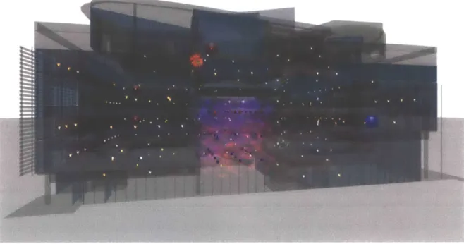
1-1 Full view of DoppelLab's representation of the Media Lab. Small or-ange flames visualize temperatures; red and blue spheres visualize

tem-perature anomalies; blue and purple fog and cubes visualizes a dense

array of temperature and humidity sensors in the building's atrium. . 13

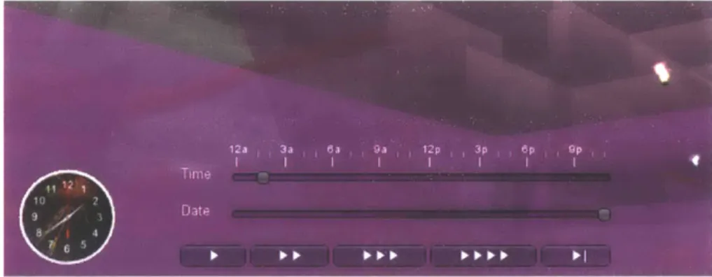
1-2 The GUI for DoppelLab's Time Machine functionality. Sliders allow

coarse and fine selection of a new time to play back data and sound

from; triangle buttons allow selection of playback speed for historical

audio (2, 3, and 4 triangles denote speedup factors of 60, 600, and

3600, resp.), the 'forward' button returns to real-time data and audio. 15

4-1 Visualization of the obfuscation process. In this example, n-grains =

4 and p-reverse = 0.5 ... ... 31

5-1 Pseudocode for main loop of granular synthesis algorithm. Numerical parameters are specified in samples; accordingly, HOP-SIZE is 30 ms, etc. 40

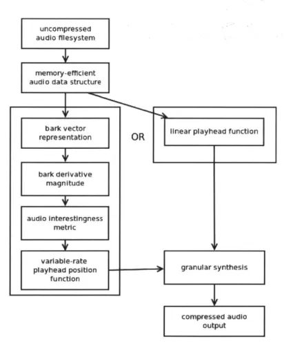
5-2 Flow diagram of audio analysis and compression algorithms . . . . 40

5-3 Analysis of 60m audio data: input and successive representations. . . 42 5-4 Comparison of outputs of constant- and variable-rate time

compres-sion. Compression ratio is 60; input is the input data from Figure 5-3 44

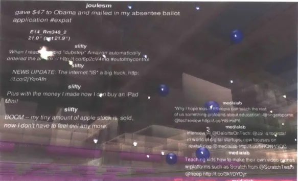
6-1 Cubes with faces on them appear when RFID tags are near sensors. . 51 6-2 Twitter streams are rendered in space according to the offic location

of their authors. They update when new tweets appear. . . . . 52

Chapter 1

Introduction

Homes and workspaces are increasingly being instrumented with dense sensor

net-works, encompassing many modalities of data, from environmental (e.g.

tempera-ture) to usage data (e.g. movement). While closed-loop systems exist for addressing

specific problems (such as temperature control), we are interested in creating a

com-prehensive interface which brings together all this complex data, and allows users to explore it and find patterns and connections between disparate kinds of data.

Graphical data visualization is a typical way to approach a problem of data display.

Data visualization is currently a very popular area, in academia, industry, and art. In Edward Tufte's seminal books, most notably The Visual Display of Quantatative Information,[35] he discusses the challenges present in visualization, and strategies

for contending with them; chief among them is the problem of 'flatland'. This refers

to the challenge of trying to visualize many-dimensional data on a two-dimensional

page or display. This problem is certainly present in the display of spatial sensor

data; these data necessarily include the three-dimensional spatial coordinates of the

sensors, in addition to time and whatever dimensions are present within the data

itself for each sensor.

In light of these difficulties, I propose the use of data sonification in order to

complement visualization of sensor data. Data sonification has been explored much

to it, the International Conference on Auditory Display,[17] and it also appears in

other converences such as the International Computer Music Conference.[18] There

also exist a very small number of well-known industry applications, such as the geiger

counter, which sonifies radiation levels using the rhythmic frequency of beeps.

A particularly interesting technique that we can use with sonification is audio

spatialization. Spatialization is the processing of audio so that it seems to be coming

from a specific location in space relative to the user. This might be achieved by using

a large number of speakers in a room so that sound can in fact be panned around in

three dimensions. However, processing techniques exist such that 3D spatialization

can be achieved even for audio played through headphones.

3D spatializated sonification is a technique particularly well suited for the display

of dense sensor network data. The spatial locations of sensors can be straightforwardly

mapped to virtual locations for spatialization. As a complement to a 3D graphical

environment, this can work particularly well, because unlike with vision, we can hear

in every direction. In this thesis, I will explore this technique of 3D spatialized

sonification as a way to convey sensor data.

This thesis builds on DoppelLab, an ongoing project of the Responsive

Environ-ments group at the MIT Media Lab.[8] DoppelLab is a cross-reality virtual

environ-ment, representing a space in the real world, and populated with visualizations of

diverse types of data, which can be explored in real time or across large spans of

past time. Currently DoppelLab uses the new MIT Media Lab (E14) building as its

test case; it pulls in temperature, humidity, sound, and movement data from existing

sensor networks in the lab, as well as sensor networks of our own creation.

Dop-pelLab uses the architectural model of the space as the framework for a 3D virtual

environment for browsing, and allows users to explore real-time data, or to play back

historical data at various speeds to see trends on different time scales; Figure 1-1

shows an example of the visualization inside the virtual space. DoppelLab aims to

provide a zoomable interface where visualizations show the large scale contours of

data from a zoomed-out view, and as the user approaches an object more detailed

Figure 1-1: Full view of DoppelLab's representation of the Media Lab. Small orange flames visualize temperatures; red and blue spheres visualize temperature anomalies; blue and purple fog and cubes visualizes a dense array of temperature and humidity sensors in the building's atrium.

inferences from the data in synthesizes and controls something in the real space;

rather, DoppelLab aims to provide a totally general browsing environment for spatial

sensor data; the hope is that by bringing together many kinds of data and allowing

the user to explore it at different speeds and vantage points, DoppelLab may allow

users to make connections themselves which might not have been anticipated by its

designers.

In this thesis, I build on DoppelLab to explore the potential of spatialized data

sonification as a way to convey spatially oriented sensor data. I explore two kinds of

data sonification: synthesized sonification of non-audio sensor data (e.g. temperature, movement and presence of people) and the use of recorded audio as sonification. I

explore in particular several issues that arise in the latter case: how to respect privacy

while using recorded audio from a shared space, and how to allow users to explore

high-level tools exist for this kind of networked audio processing application exist, so my

work also involved the design and implementation of this system.

The resulting system offers several ways to explore data through audio, through

the existing DoppelLab user interface. Seven microphone streams from the public

areas in the Media Lab, obfuscated for privacy, are played back in the application, spatialized according to the locations of their recording in the real space. As with

the other data in DoppelLab, the user may explore real-time or historical audio. The

default mode is to play real-time audio (within several seconds of strictly real-time, as a result of buffering in various parts of the system). DoppelLab provides a slider

interface by which the user can select a historical time from which to play back

datal-2; with my audio system, the recorded audio streams also play back archived audio

from the requested historical time (at the time of this writing, the audio archive goes

back several months and is continuing to accumulate.) Additionally, like the rest of

DoppelLab, the program allows playback of archived audio at faster-than-real-time

rates, using an audio time-compression algorithm of our creation. To protect privacy

of users in the space, we obfuscate audio data at the nodes where it is recorded. In

addition to this recorded audio system, I have implemented a number of synthesized

sonifications of other building data; this sonification work is basic, but it allows us

to explore the issues involved in sonifying spatially-oriented data, and doing so in

conjunction with a graphical 3D interface.

In Chapter 2, I will discuss prior art in related areas, such as sonification, audio

privacy, and audio analysis. In Chapter 3, I will give a brief review of what

spatial-ization is, how it can be done, and what solutions I use in my work. In Chapter 4, I will discuss how my work navigates data privacy issues which come with using

recorded audio. In Chapter 5, I will describe techniques I used for distilling down

large amounts of audio data, in order to make it easier to explore. In Chapter 6, I

will discuss several synthesized sonifications of non-audio data that I made. Finally, in Chapter 7, I address the design and implementation of the software system which

Figure 1-2: The GUI for DoppelLab's Time Machine functionality. Sliders allow coarse and fine selection of a new time to play back data and sound from; triangle buttons allow selection of playback speed for historical audio (2, 3, and 4 triangles denote speedup factors of 60, 600, and 3600, resp.), the 'forward' button returns to real-time data and audio.

Chapter 2

Related Work

2.1

Synthesized Data Sonification

Data Sonification is an active area of research, with work on perception of sonification, creation of tools for sonification, and creation of novel sonifications themselves. My work on DoppelLab relies on these perceptual studies as a basis for the effectiveness of musical sonification in general, and specifically some techniques such as pitch mapping and multi-channel techniques.

User studies have quantatatively shown the effectiveness of certain kinds of data sonifications for understanding features of graphs, both in seeing and blind users. Brown and Brewster performed a user study[5] where blind users were played soni-fications which mapped functions of one variable to pitch, and were asked to draw graphs of the data; high accuracy was measured in terms of whether the drawings included features from the data which was sonified. In their work Musical versus Visual Graphs[11], Flowers and Hauer show that simple time-series visualization and pitch-mapping sonification were similarly effective for perception of data features such as slope and shape in time-series data.

Based on a number of perceptual studies like the above, Brown et al. published[6] a set of guidelines for sonification. The guidelines concern sonifications of one or

several variables as a function of time, targeting blind users specifically. Among other guidelines, they recommend mapping the dependent variable to pitch in

gen-eral, and for multiple variables they recommend stereo separation and allowing the

user to change relative amplitude levels; these latter two qualities can be effectively

accomplished through spatialization.

In terms of specific sonification designs, we are particularly interested in the prior

work which specifically concerns spatial data, audio spatialization, or both. This is

discussed in Section 2.2.

2.2

Spatialized Data Sonification

An early precedent for this work can be found in R. Bargar's work in creating

inter-active sound for the CAVE system, which augments a graphical virtual environment

with spatialized sounds. [3] Spatialization is accomplished using reverberation and

de-lay and can be performed using speakers or headphones. This system is probably

restricted by performance issues which are no longer problematic; for example, it

can only spatialize 4 sound sources; the ability to spatialize many more than that is

essential for our ability to sonify large sensor arrays.

Hunt and Hermanns Importance of Interaction

[15]

that correspond to natural acoustic phenomena (e.g. when sound is produced by

striking an object, a harder strike produces a louder sound.) 3D spatialization, a

technique which I make heavy use of, is a good example of such a real-time feedback

phenomenon. A main design criterion of my system is that it performs spatialization

on the client, rather than the server; this removes network latency as a significant

potential source of latency in the interaction, and allows for more realistic, real-time

feedback.

Some work on sonification with an emphasis on spatialization exists. In their

sonification of a Mixed-Reality Enfironment[21], Le Groux et al. sonify the positions

of participants in the system, but spatialization itself is not used to directly convey

spatial information, but as another effect to make the piece more immersive.

work where either the data is spatial, the sonification uses spatialization, or both. One relevant conclusion they note is that spatialized sonification can enhance visualization of the same or related data.

Many of the spatialized sonifications of spatial data mentioned in [24] use data with fewer than three spatial dimensions; for example, for example, Franklin and Roberts[12] sonify pie chart data using horizontal spatialization; Zhao et al. [40] sonify geographical data which has two spatial dimensions.

Andrea Polli's Atmospherics/Weather Works[30] is a striking and ambitious ex-ample of spatialized sonification of data with three spatial dimensions. This work sonifies data from a storm, over a 24 hour period. It includes multiple data

param-eters, including pressure, humidity, and wind speed, sampled in a three-dimensional grid spanning the atmosphere and a 1000km2 horizontal area. All parameters were

mapped to pitch, with different timbres differentiating kinds of data; a multi-speaker setup was used to spatialize the data according to heights at which it was sampled.

2.3

Privacy

Previous work from our group, the SPINNER project, [20] addresses the importance of privacy in distributed sensor networks, particularly with respect to audio and video data. SPINNER uses an opt-in model for sharing of audio and video data, where it requires building occupants to wear a badge, and recording is enabled only if a badge is in range and the user's preferences are set accordingly. If these conditions do not hold, or if recording is manually interrupted (by design, there are a number of easy ways to do this), audio and video recording is disabled entirely. This comprises a viable model

for privacy, but in DoppelLab, we would like to avoid requiring users to wear badges, and losing significant windows of data, if possible. DoppelLab is primarily interested

in audio as a way to sonify the usage of a space, especially compressed over large time

spans, the semantic content of recorded speech is not of interest to us. As this is the

primary sensitive aspect of audio data, we address the privacy issue by obfuscating

and timbre to the greatest possible extent.

Some work exists on obfuscating speech content of audio while preserving timbre. Chris Schmandt's ListenIn [32] system uses audio for domestic monitoring among family members or caregivers. ListenIn detects speech, and scrambles the audio by shuffling short buffers whenever speech is detected, aiming to make speech unintelli-gible but otherwise preserve timbre. More recent work by Chen et al. [7] alters vowel sounds in speech, and includes a user study which demonstrates that it significantly reduces intelligibility while leaving concurrent non-speech sounds recognizable. While these works present interesting methods, they do not address the question of whether a third party could process the obfuscated audio and restore intelligibility. In [32], this is reasonable because the application is meant to be a closed system where data is shared among a small number of individuals; in [7], applications are not discussed.

In their work on Minimal-Impact Audio-Based Personal Archives, Lee and Ellis[9] address the issue of obfuscating audio in a way that would be difficult to reverse. Their application involves people carring portable recorders with them, rather than recording a space at fixed locations, but in both these applications, obfuscation which is difficult to reverse is important. Their method is similar to the one in [32]; they classify the audio as speech or non-speech, and then obfuscate the speech; in this case obfuscation is performed by shuffling, reversing, and cross-fading between short windows of audio. They claim that given certain parameters (shuffling 50ms win-dows over a radius of Is, with "large" overlap between adjacent frames) would make reversing the obfuscation "virtually impossible". They note that this kind of obfus-cation should leave spectral features in the audible range largely untouched, so that audio analysis would not be disrupted. For their application, Lee and Ellis claim that unobfuscated speech is the most interesting part of the recorded audio; they cite among other reasons a "nostalgia" appeal in listening to old conversations. They dis-cuss the possibility of turning off obfuscation for speakers who have given the system

2.4

Audio Analysis and Time Compression

In this project, I use recorded audio from the space in order to help convey the usage of the space. In particular, I archive all that data and try to make it easy for users

to explore the archived data efficiently. My general strategy for doing this is to allow

users to seek around the audio archives and listen to versions which are radically

time-compressed, by factors ranging from 60 to 3600. There exist large bodies of

work related to time-compressing audio data, and exploring large bodies of audio

data, but the main areas here differ from what this thesis attempts in significant

ways.

There exists a large area of audio time-compression and content-aware time

com-pression work, but it is focused on time-compressing recorded speech. This work

differs from mine first in that in order to achieve this goal, relatively small

com-pression ratios are used- generally less than 3. A bigger difference is that with

this specific objective, there exist analysis techniques, based on speech structure, which can guide compression more effectively than a general (non-speech-related)

al-gorithm could; also, there are more specific metrics for evaluation, based on speech

comprehension. [26] [14]

Music Information Retrieval (MIR) is a major area of research which aims to

help users understand huge bodies of audio data. MIR, though, is typically based on

search, while DoppelLab's aim is primarily discovery.

One piece of work with more direct relevance is Tarrat-Masso's work in [34], which

uses spectral analysis to guide audio compression. This work, too, has a more specific

problem domain than DoppelLab; it concerns time-compression for music production.

However, the analysis and resynthesis are decoupled, and the analysis isn't specific

to musical inputs. The analysis is based on Image Seam-Carving, [2] involves

calcu-lating an energy map of the spectrogram (a three-dimensional representation of an

audio sequence, which plots power as a function of time and frequency) of the audio, and then applying the most compression to times when there is the least amount

although I build on it in several ways, including using a perceptual weighting of the audio spectrum.

2.5

DoppelLab

This thesis builds on the Responsive Environments Group's ongoing project, DoppelLab[8], which we introduced in Chapter 1. In this thesis I am exploring in particular ways to use sonification to complement 3D graphical visualizations, and to do so I will integrate my implementation with the existing DoppelLab system. Here I will review how DoppelLab approaches data visualizations, and how its system is designed.

DoppelLab aggregates and visualizes data from a large and still growing set of sensor modalities within the MIT Media Lab. An architectural model of the Media Lab serves as an anchor for these visualizations; all data visualizations are localized in virtual space according to the locations of their corresponding sensors in physical space. The building's structures themselves are by default visible but transparent, so that they highlight the physical locations of the data but do not obstruct the view. A common thread of the visualizations is the idea of micro and macro design; visualiza-tions consist primarily of multiples of simple geometric forms, such that differences across sensors can be seen from a view of the entire lab, but display more detailed quantatative information when the user zooms in or clicks on them. One visualiza-tion shows temperatures throughout the lab based on over two hundred thermostats; warmer or cooler colors represent relative temperatures; numerical temperatures are displayed upon zooming. Another visualization shows both audio and motion lev-els in about ten locations; the audio level visualization uses the form and colors of familiar audio level meters; this visualization itself also oscillates, as if blown by a gust of wind, to indicate motion. Some visualizations show higher-order phenomena based on inferences made on more basic sensor data. For example, significant trends in motion and audio levels at a location can indicate the arrival or dispersal of a social gathering; DoppelLab shows clouds of upward or downward arrows when this happens.

A major part of DoppelLab's visualization power is an interface for exploring time. By default, DoppelLab shows real-time data. A heads-up display (HUD) (pictured in

Figure 1-2) allows for exploration of past data; at the time of this writing, most of the data is archived for around one year. Using the HUD, a user can select a past time to visit, and once in historical data mode, the user can select among three faster-than-real-time speeds at which to view data. These speeds allow the user to view large-scale patterns which would not otherwise be apparent; for example, at the fastest speed-up of one hour per second, it is easy to see the temperature anomaly visualizations appear every night in a periodic fashion, indicating that the air conditioning system is overactive at these times.

DoppelLab's client is built with the Unity game engine[37]. Unity allows for rapid creation of visualizations, using a combination of a graphical user interface and C# and a JavaScript-based scripting language. The client has a main loop which queries the DoppelLab server every few seconds, receives sensor data from it in XML, parses the XML, and calls the appropriate callback functions to update the visualizations. The client maintains state indicating the current time and speed at which the user is viewing data, and that information is included in the server queries.

The DoppelLab server is written using Python and a MySQL database. The server has scripts which poll sensor data sources and aggregate the data in the central database. The server also includes a web server which responds to queries from DoppelLab clients, and returns the appropriate data from the database; for queries from clients running through historical data at a fast rate, the server computes and returns averages over correspondingly large ranges of data.

Chapter 3

Spatialization

Spatialization is the processing of audio to give the impression that it is coming from a specific location in space relative to the listener. In spatialization, we usually discuss a listener, which represents the simulated position and angle of the listener's head in virtual space, and one or more sources, which represent different mono audio sources, each with its own simulated position in space.

One way to implement spatialization is to set up many speakers so that sound

can be panned between them; a typical way to do this in a sound installation is to have eight speakers placed in the eight corners of a rectangular room. However, to

make it easier for more people to test our system, we focus mainly on using audio-processing-based spatialization which will work with a headphone setup.

This thesis is about way to apply spatialization, and thus does not focus on the

implementation of spatialization itself. This chapter includes a brief discussion of

what spatialization is and how it is often performed, and a discussion of the tools used in our implementation.

3.1

Review of Spatialization Techniques

There exist many methods which may be combined to implement sonification; within

these there is a spectrum of levels of sophistication, which can lead to more or less

The most basic way to implement spatialization is with amplitude attenuation

and panning between the ears. Amplitude is attenuated as a function of distance

from the source, according to a variety of models. Panning between right and left

channels simulates the angle between the source position and the listener's facing.

Spatialization engines often offer a variety of amplitude rolloff functions to the

programmer. An inverse distance model, which corresponds with inverse-square

at-tenuation of sound intensity, is typically offered; for example, it is the default option

in OpenAL[28], the spatialization engine used in this thesis[27]. Other models are

of-ten available, though; for example, both OpenAL and Unity3D have an option where

gain decreases linearly with distance, and Unity also has an option where the game

designer can draw in an arbitrary gain function using the GUI[38]. These options

exist because simple spatialization models fail to take into account other real-world

factors, so a designer might find that cutting off gain artificially quickly at some point

is a suitable approximation of other real-world factors, such as sound obstruction and

other ambient noise. Another common modification is 'clamping', which imposes an

artificial maximum on the gain function; this is important because in simple game

models we might be able to get arbitrarily close to a sound source, which if an inverse

gain model is used, can result in arbirarily high gain.

Panning and attenuation can offer us some cues in terms of left-right source

move-ment relative to the head, and relative distance from the head, but other techniques

are necessary in order to achieve full 3D spatialization. One common technique is

the use of head-related transfer functions (HRTF). The HRTF is an

experimentally-measured transfer function, which attempts to imitate the way the shape of the

listener's outer ears, head, and torso filter audio frequencies that come from different

directions relative to the listener.[4] The effectiveness of this technique is limited by

the extent to which a given listener's anatomy differs from the model used in the

cre-ation of the HRTF; however, it has been shown that listeners can adapt to different

HRTFs over time.[16]

Simpler kinds of filtering can also be used to achieve distance cues. In particular, applying a low-pass filter to sounds that are farther away simulates the fact that

higher frequencies attenuate more over these distances.

Spatialization can also be improved by using reverberation effects. Sound pro-cessed using a reverb algorithm is typical mixed with unpropro-cessed sound in a "wet/dry mix", to simulate reflected and direct sound. Using relatively more dry sound sim-ulates a sound closer to the listener. This can be done more effectively if a physical model of the room that the listener is in is used. Using effects such as these last two in addition to attenuation is particularly important for displaying distance; otherwise, it is unclear whether a sound is closer or just louder.

3.2

Using Spatialization in DoppelLab

One of the main design decisions I made in the DoppelLab sonification system was to perform spatialization on the client and not remotely; I discuss this issue more in Chapter 7. The client for display of recorded audio data is implemented in C as a

Unity plugin. In the recorded audio sonification system, spatialization is performed using OpenAL[27]. OpenAL is cross-platform library for 3D audio and provides a simple interface in the style of the ubiquitous graphics library OpenGL. The spec-ification of OpenAL states that the exact method of spatialization (e.g. HRTF) is implementation- and hardware-dependent[28].

I use the default distance attenuation model in OpenAL; this scales audio by a

gain factor proportional to the inverse of the distance; since sound intensity is pro-portional to the square of gain, this corresponds correctly to the inverse square law of sound intensity in physics. We then set a reference distance which sets OpenAL's dis-tance scale correctly according to how DoppelLab communicates listener and source information to it. The result is that audio streams' volumes are proportional to how

they would be in the real world if no obstruction or other ambient sounds existed. These qualities are of course not maximally realistic, but they make some conceptual sense with the graphical representation in DoppelLab. By default, the architectural

model in DoppelLab is rendered to be visible but transparent. The transparency of

toggling of the building's walls as acoustic obstructions.

The synthesized data sonifications in this thesis were implemented as Max/MSP patches[22]. For prototyping purposes, spatialization of those sounds is implemented within Max using a custom spatializer, which does a primitive spatialization using panning and amplitude attenuation. Section 6.1 contains more discussion of this issue.

Chapter 4

Privacy

The goal of obfuscating the audio streams is to protect the privacy of the occupants

of the space while keeping as much useful data as possible. We consider useful data

to be data which characterizes the activity happening in the space; for example, we should be able to hear if there is a lecture, a small conversation, or a loud gathering happening; we should be able to hear elevators, ping-pong games, and the clattering

of silverware. To this end, we use a combination of randomized shuffling and reversing

of grains (short sections of audio, on the order or 100ms) on the time scale of spoken

syllables.

4.1

Obfuscation

In order to prevent the privacy violation of recording, storing, and transmitting peo-ples' speech in a shared space, I aim to obfuscate recorded audio streams directly at the nodes where they are recorded. By 'obfuscate', I mean process the audio so that no spoken language can be understood. It is important that we perform this processing on the machines where audio is being recorded; otherwise we would be

transmitting unprocessed audio over the network, where it could be intercepted by

a third party. Also, we archive all of our audio data so that our application can

allow users to explore data over larger time scales; it is important to only store

to our database, and from actual developers on the DoppelLab system. Encryption

would not work as well as obfuscation for protecting the data during transmission

and storage, because DoppelLab would have to be able to decrypt the data for audio

processing and display, and thus DoppelLab developers would be able to gain access

to the unencrypted audio.

For our obfuscation algorithm we have several requirements. We would like it to

be unintelligible; that is, listeners cannot understand significant segments of it (i.e.

more than an occasional word or two.) We could like it to preserve timbre, both of

speech, and of environmental sounds, including the shape of transient sounds, and

e.g. the number of speakers). Finally, we would like it to be difficult to reverse, or

deobfuscate; we will discuss this idea further in Section 4.1.2.

Another requirement for the obfuscation algorithm is computational efficiency. In

our current setup, the node machines where audio is recorded are primarily deployed

for a different purposel; therefore, we are not entitled to run particularly

computation-intensive jobs on them. While that constraint may be peculiar to this particular

deployment, it is reasonable in general that we would need an inexpensive algorithm.

If we wanted to achieve higher microphone density, or if we were deploying in a

situation where we didn't have access to computers around the space, we might want

to run the algorithm on a microcontroller.

4.1.1

Algorithm

Our algorithm works in a similar way to the one presented in [32], but attempts to

improve on timbral preservation. To that end, we shuffle fewer, larger grains, instead

of a larger number of smaller grains. To offset the increase in intelligibility that this

causes, we randomly reverse some of the grains. We also significantly overlap and

crossfade between sequenced grains, to create a smoother sound.

The algorithm works as follows. We maintain a buffer of the n-grains most

recent grains of audio, with each grain grain-length + f ade-length milliseconds

'The node machines' primary purpose is to run instances of the Media Lab's Glass Infrastructure. [13]

Figure 4-1: Visualization of the obfuscation process. In this example, n-grains = 4 and p-reverse = 0.5

long, overlapping by fade-length ms. At each step, we record a new grain of audio from the microphone, and then discard the oldest grain. We then read a random

grain from the buffer. With probability p-reverse, we reverse the audio we have just read. We then sequence that grain; i.e. we write it to the output, crossfading it with

the last fade-length milliseconds of output. Figure 4-1 visualizes how the algorithm acts on several grains of data.

Currently the algorithm is deployed with the following parameters: n-grains =

3, p-reverse = 0.6, grain-length = 8192, fade-length = 2048, where the latter two parameters are in terms of PCM samples. Logarithmic crossfades are used to keep constant power during crossfades; this sounds less choppy aesthetically and makes it less obvious for a decoder to detect where exactly grain transitions occur; as an ex-ception, we perform linear crossfades when the transition would be in-phase. These parameters were chosen based on optimizing for quality of timbre while maintaining unintelligibility. However, prior work such as [9] suggests that more aggressive scram-bling, i.e. shuffling among more grains of smaller size, while maintaining significant crossfades, would provide more of a guarantee against an eavesdropper reversing the

algorithm; accordingly, we intend to revisit these parameters soon.

The audio output of this algorithm is unintelligible, by observation, and it

pre-serves the timbre of many environmental sounds. For example, the distinctive bell

sound of the Media Lab's elevators is preserved nearly perfectly- since this is a

rela-tively constant tone which lasts several seconds, shuffling grains which are significantly

prop-erty of the obfuscation algorithm: since we only shuffle grains of a certain length, significantly longer and shorter sounds are largely unaffected. Significant changes in the tone of speech can be heard; laughter, for example, is often recognizable. Very short sounds, such as the percussive tones of a ping-pong game in the atrium, are also recognizable. Such short sounds are sometimes less clear since the reversal can affect them, but if a sound repeatedly occurs (such as, again, ping-pong hits), probabilistic independence of grain reversal makes a near-guarantee that many instances will be played forward.

4.1.2

Deobfuscation

In the interest of privacy, it is important not only that our obfuscated audio is un-intelligible, but that it is difficult to reverse the obfuscation procedure. Otherwise, a user could download and archive the audio streams and attempt to process them so that the original audio is intelligible; either by manipulating it manually using an audio editor, or by writing a program which analyses the audio and attempts to reconstruct contiguous speech passages.

Currently, we do not know of a way to prove that the obfuscation would be prac-tically impossible to de-obfuscate, or even exactly what that condition would mean. We can make some conjectures. Reversal of the algorithm, if possible, would probably involve either spectrally analyzing grains and finding grain boundaries which seemed to match up, or applying phoneme detection and then using a phonetic model to

look for common phoneme sequences. Significant crossfading will make both of these approaches difficult, particularly the first one- with a large logarithmic crossfade, as we get near the edge of a grain, the spectrum of that grain will be mixed close to equally with the spectrum of the next grain; if the time scale on which syllables change is similar to the time scale of the crossfade size, it will be difficult to undo that corruption. If cross-fades comprise a large proportion of the duration of a grain, it will be more difficult for phoneme detectors to identify phonemes.

Another property of the algorithm that we note is that if we randomly sequence grains from a set of the most recent N grains, then a given grain will be in the set

during N sequencing intervals, and then the probability of that grain never being

played is ((N - 1)/N)N. If we maintain a set of 3 grains, this probability is

approx-imately 0.30; if the set has 10 or 20 grains, the probability is approxapprox-imately 0.35

or 0.36. Thus, approximately one of every three grains will be dropped. Thus, for

an algorithm reversing this process, only short contiguous sequences of grains would

even exist, and then if those were all identified, the algorithm would have do recognize

Chapter 5

Time Compression of Audio Data

One of DoppelLab's main features is the ability to explore historical data on

faster-than-real-time time scales (up to several thousand times) in order to understand

larger-scale patterns. My focus has been on using recorded audio data from the

Media Lab to provide information about activity within the space. Unlike many

graphical visualizations, which can be sped up simply by fetching sequential data at

a higher rate, audio data is not trivially sped up. Since we perceive audio data in

terms of frequencies, speeding up the data by the kind of factors we deal with in

DoppelLab (e.g. 60 to 3600) would bring the data out of the human range of hearing.

I have designed and implemented an algorithm for speeding up audio data for this

application, which has two parts: one part uses a method called granular synthesis

(defined in Section 5.2), which is used to resynthesize audio from any time offset in

the source audio without altering its frequency; the other part determines which input

audio we resynthesize from. I experimented with both traversing the input file at a

constant speed, and traversing at a variable speed, where I spend more time on audio

which has more interesting features. I perform some spectral analysis to determine

5.1

Analysis

DoppelLab involves speeding up audio by several orders of magnitude; in the current application, by factors ranging from 60 to 3600. To compress sound by such a high ratio, it is necessary to discard some data. If we proceed through the sound at a constant rate, we will lose information equally from all sections of the data. If we can identify sections of the data which are more interesting to us, we can apply less steep compression to those sections, making it more likely that they will still be recognizable and meaningful to the listener.

Of course, the question of which audio is more interesting is very open-ended.

Given the exploratory nature of DoppelLab, we do not want to restrict the user to a specific type of event, such as human speech or activity. Also, we do not want to simply select audio that has more noise or activity, as this could create an innaccurate

representation of certain data. For example, if an interval of time has both loud conversation and silence, we would like to represent both. To accomplish this, we use a perceptual frequency scale to get a compact representation of the audio features that humans perceive in greatest detail. We then look at the amount of change in

this representation over time, and bias the compression to preserve these times of transition, and apply more compression to times when the sound is more constant.

5.1.1 Bark Frequency Scale

The Bark frequency scale, proposed by E. Zwicker, is a subdivision of the audible frequency range into 24 distinct frequency bands, corresponding to the experimentally

measured critical bands of human hearing. The division into these critical bands is thought to be closely related to the perception of loudness, phase, and other auditory

phenomena. [41]

5.1.2

Audio Interestingness Metric

Given a Bark vector as a perceptually-scaled representation of the audio spectrum, we consider the magnitude of the derivative (or difference between vectors from two

consecutive windows) of the Bark vector as a metric representing how much change is happening in the audio signal. Since the Bark vector has 24 components

correspond-ing to frequency bands, measurcorrespond-ing the magnitude of the derivative will capture many meaningful changes in ambient sound as a listener would perceive it; e.g. changing

pitch of a pitched sound, introduction of a new frequency, change in volume, increase

or decrease in noisiness of the signal. Therefore the magnitude of the derivative

con-stitutes a metric for how much perceptible change is happening; for lack of a more

lexically pleasing name I refer to it as the "Interestingness metric".

To compute the Interestingness metric over a signal, I compute the FFT at

con-tiguous, nonoverlapping windows of some window size. From the FFT, which has

many frequency bands compared to the Bark (i.e. thousands or more), we need only

sum the power of each frequency between successive Bark band edges to get the power

in each Bark band.

Note that the window size over which we compute the Bark vectors is critically

important, and is related to the time-scale of events that we could expect the listener

to perceive at given time-compression ratios. For example, suppose we are

compress-ing an hour of audio into a minute. We might be able to show that a conversation

took place over several minutes. However, we probably don't care about the sonic

details of every phrase or sentence- we only have a minute in total, and there may

be other interesting events which will get encoded. If we use a 'typical' FFT window

size for audio analysis, e.g. 1024 or 4096 samples, this will register significant spectral

change as the conversants' syllables change and their sentences begin and end. On

the other hand, if we use a larger window size, e.g. 10 seconds or a minute, the Bark

vector will be averaged over this time, and will smooth over the small sonic changes

that happen during a conversation. However, it will register change on the beginning

or end of a short conversation.

To interface with our granular synthesizer, we want to provide a map indicating, for a given time offset in the audio output, where to draw a sample from in the audio

input. Given the interestingness metric, we would like to spend the largest amount of

the desired playhead speed. We then integrate with respect to time to get something proportional to how the playhead position in the input file should vary with respect to position in the output file. Since the map's domain is output file position and the range is input file position, and the beginnings and ends of the input and output file should match up (since we want to compress the entire input and nothing more, and we want to move through it monotonically), we scale the map so that the domain and range correspond respectively to output file length and input file length.

5.2

Synthesis

This section describes the algorithm which synthesizes time-compressed audio. We use a technique called granular synthesis (detailed in the following sections), which allows us to resynthesize audio from a recording and warp playback speed while not altering frequency.

5.2.1

Granular Synthesis

Granular synthesis[31] is a type of audio synthesis that involves creating sounds by sequencing and layering many short 'grains', or samples typically of duration 1 to

100 ms. Sometimes grains are synthesized; we use a technique called "time

granula-tion", in which grains are created by sampling an existing audio source. By sampling grains around a specific time in the audio input, or a 'playhead', we can capture the timbre of that moment in the audio. We can then extend that moment arbitrarily,

by keeping the playhead in that location.

Time granulation employs a variety of techniques to avoid artifacts when resynthe-sizing audio (or create them, at the programmer's discretion.) A naive implementa-tion, simply creating a short loop at the location of the playhead, will have artifacts; longer loops will create an audible rhythmic pulsing, and shorter loops, where the period of repetition is above 20Hz or so, will produce an audible low-frequency hum. Granular synthesis solves this problem by windowing and layering together many short samples, or 'grains', using some randomness in the length and start time in

order to avoid artifacts.

5.2.2

Compression Algorithm

I tried two approaches to audio time compression using granular synthesis. In the

first, the playhead moves through the input file at a constant speed. In the second,

I try to identify moments of interest in the audio (using the analysis described in

Section 5.1) and bias the playhead to move relatively more slowly during those parts, so that the interesting moments of transition can be played back with higher fidelity, and longer, monotonous sections can be passed over quickly.

The compressor program is written so that these different playback patterns can

easily be swapped in and out. The compressor takes as an argument a 'playhead

map'; a function which indicates, for a given moment in the output file, where the

granular synthesis playhead in the input file should be. So for the constant-speed

playback, the playhead map is a linear function which returns an offset proportional

to the input by the compression ratio. For the variable-speed playback, then, the

offset map should be a monotonically increasing function which increases more slowly

during areas of interest in the audio. In Section 5.1.2 I describe how that map is

created.

During synthesis, grains are sampled at the location of the playhead, with a

ran-dom duration within a specified range. Grains are then multiplied by a three-stage

linear window to avoid clicks, and added to the audio output. Figure 5-1 shows

pseu-docode for the main loop of the compression algorithm, given a playhead map. (I

use python/numpy-style syntax where array [start : end] can be used to access

a subarray of an array, and operators like += distribute element-wise if operands are

arrays.) Figure 5-2 shows a flow chart of how the analysis and synthesis comprise the

HOPSIZE, MINGRAIN MAX-GRAIN, OUTPUTLENGTH = [0.03, 0.1, 0.5, 60] * 44100

outputoffset = 0

while output-offset < OUTPUT-LENGTH:

grainsize = random int in range (MINGRAIN, MAXGRAIN)

new-grain = audio-in[playhead-map(output-offset)

playhead.map(output-offset) + grain-size]

apply three-stage linear window to new-grain

audioout[outputoffset outputoffset + grain-size]

+= new-grain

output-offset += HOPSIZE

Figure 5-1: Pseudocode for main loop of granular synthesis algorithm. Numerical parameters are specified in samples; accordingly, HOPSIZE is 30 ins, etc.

uncompressed audio filesystemJ

memory-efficient audio data structure

beark ectton linear playhead function

bark derivative magnitude

audio interestingness

metric

variable-rate

playhead position granular synthesis function

compressed audio

output

5.3

Results

In this section I show some data from intermediate steps and output from the time

compression algorithms, and discuss some informal testing by myself and a few

col-leagues.

5.3.1

Data

My process for variable-rate time compression involves a number of steps; I will use

some data to demonstrate how it works. Figure 5-3 shows a section of input data and

successive representations, for compression ratio 60. The input data are chosen as an

instance where we have some interesting events which we would like to show in higher

resolution; the beginning is mostly quiet, we have a few brief periods when people

walk by and talk, and then near the end the beginning of a musical jam session can be

heard. All four subfigures are on equivalent time scales, so corresponding data line up

vertically. The first subfigure is a spectrogram showing the 60 minutes of input data;

a spectrogram is a plot which shows successive windows of spectral representation

over a longer signal; power is mapped to color. The second subfigure shows, for

successive windows, the values of the Bark vector. The third subfigure shows the

Interestingness metric over the same data, or the magnitude of the derivative of the

Bark vector; the fourth shows the playhead map, which indicates the location in the

input file at which the granular synthesizer should be sampling from for each moment

in the output file. Note the several more flat regions; these are moments of interest

where the playhead spends more time.

Figure 5-4 shows spectrograms of the minute-long audio outputs from

contant-and variable-rate time compression, given the hour of input data shown in Figure

5-3. The first image, predictably, looks similar to the original data in the first subfigure

in Figure 5-3, since we are compressing using a constant speed, and since the images

don't have resolution to show the details in the hour-long sample which don't exist in

the compressed version. In the second subfigure, as intended, we can see many of the

Spectrogram of original audio (window size 2e16 samples) 12000 10000-8000 U C 6000 r 4000-LL 2000 0 500 1000 1500 2000 2500 3000 3500 Time (seconds)

Bark vectors of ori inal audio (window size 2e19 samples)

20

15

10

0 50 100 150 200 250 30(

Bark window number

4.0 Ie1O Bark derivative metric

3.5-> 3.0-L 2.5- 2.0-.u 1.5- 1.0-E 0.5 O

0.0

0

S1.l Playhead position map

1.6

a

output time offset (samples) 42

audio. The "event" annotations point out a few moments where we can clearly see the

same audio feature showing up in both outputs, based on the spectral characteristics.

In particular, with "event B", we note that the event, which is brief, barely shows

up in the first subfigure, and is even more difficult to see in the input data. In

the second subfigure though, the event is bigger and darker, and farther away from

the peak immediately to the left of it. Similarly, with "event C", we see a pair

of short, dark peaks, and some lighter peaks to their left; in the second subfigure, all this dense activity is more spread out in time. These two examples illustrate

the variable-rate compression algorithm dwelling on events with more change, or

with unusual frequencies, over relatively longer periods of time, thus showing them

in higher resolution. This is at the expense of more monotonous sections, like the

several more static periods early in these spectrograms.

Note that slight variations in the outputs of the different algorithms (e.g. in

Figure 5-4) can appear apart from the main time-warping effects. This can result

from the randomized nature of the granular synthesis algorithm; since grain length is

randomized within a range, successive longer or shorter grains can produce a small

fluctuation in intensity. In addition, large-scale changes in how the playhead for grain

sampling moves through the input file will affect, on a grain-sized scale, exactly which

grains in the input are sampled.

5.3.2

Testing

The first evaluation I did of this compression was testing it myself. In general, I was

surprised by how good even the constant-rate compression sounded; because of the

granular synthesis, social gatherings and music in particular were often smoothed into

a sped-up, but still recognizable, soundscape. When comparing the two methods side

by side on the same data, I did find that the variable-rate compression sounded like

it spread out activity in the audio more. The effect was particularly noticeable on

relatively short sounds; with constant-rate compression, these sounds could come out

sounding clipped, probably having been only sampled in one or a few grains. In the

Constant-Rate Compressed Audio

[ent

Time (seconds)

Variable-Rate Compressed Audio

7nnn.

Ient

B

-vent A

Time (seconds)

Figure 5-4: Comparison of data from Figure 5-3

outputs of constant- and variable-rate time compression. Compression ratio is 60; input is the input

N I U w 0* 0) U->1 U 10000 8000 6000 4000 2000 0 10000 8000 6000 4000 2000

I