Do Markets Mitigate
Misperceptions of Feedback in Dynamic Tasks? John D. Sterman, 617/253-1951
MIT Sloan School of Management and
Christian Kampmann, 45-4-288-1611 Technical University of Denmark
Do Markets Mitigate
Misperceptions of Feedback in Dynamic Tasks?
Christian Kampmann John D. Sterman
Sloan School of Management, E52-562 Massachusetts Institute of Technology
Cambridge, MA 02139
ABSTRACT
We test the ability of market forces to mitigate the dysfunctional effects of systematic 'misperceptions of feedback' - mental models which ignore critical elements of a task's feedback structure - demonstrated in prior experiments. We create a simulated multiple-agent market under two feedback complexity conditions (simple and complex) and three market institutions (fixed, market clearing, and posted prices). While performance relative to optimal in the market clearing and posted price conditions was better than the
fixed price condition, complexity significantly degraded relative performance in all conditions. Markets moderate but do not eliminate the negative impact of misperceptions of feedback.
To be presented at the 1992 International System Dynamics Conference, University of Utrecht, The Netherlands, 14-17 July. Please direct correspondence to John Sterman (address above or [email protected]).
D-4278 2
Markets and Dynamic Decision Making
Recent studies show decision making in complex dynamic environments is poor relative to normative standards, or even simple decision rules, especially when decisions have indirect, delayed, nonlinear, and multiple feedback effects (Diehl 1992, Sterman 1989a, 1989b, Kleinmuntz 1985, Brehmer 1990, Smith, Suchanek, and Williams 1988; Funke 1991 reviews the large literature of the 'German School' led by D6rner, Funke, and colleagues). Sterman (1989a, 1989b) argues that the mental models people use to guide their decisions in dynamic settings are flawed in specific ways: that they tend to ignore feedback processes which cause sieffects, that they fail to appreciate time de-lays between action and response and in the reporting of information, that stock and flow dynamics are not accounted for properly, and that they are insensitive to nonlinearities which may cause the relative importance of different feedback processes to change en-dogenously as a system evolves. Sterman argued that such "misperceptions of feed-back" generate systematically dysfunctional behavior in dynamically complex settings.
Many economists, however, have questioned the relevance of such laboratory evidence, arguing that market forces compensate for individual departures from rational-ity through adaptation, arbitrage, learning, and competitive selection (Hogarth and Reder 1987). So far, however, there have been no attempts to test whether the misperceptions of feedback phenomenon seen in dynamic tasks persists in the presence of market mech-anisms and financial incentives. Though there are many dynamic decision making tasks in the real world for which no or only poorly functioning markets exist (e.g. real-time process control, organizational settings such as schools and bureaucracies, and environ-mental dynamics, etc.), the ability of market forces to mitigate individual departures from rationality in dynamic tasks is a critical area of research for psychology, economics, and system dynamics.
Overview of Experimental Design
The research questions addressed here are: 1) To what extent can market mecha-nisms and financial incentives alleviate the problems observed in non-market dynamic decision making experiments? 2) What is the effect of feedback complexity on market behavior and performance?
Most studies in experimental economics have involved markets with relatively simple dynamic structure. In particular, markets are usually "reset" each period so that past decisions do not influence current or future options (Smith 1982; Plott 1982). Yet human performance degrades significantly in the presence of delays, accumulations (stocks and flows), non-linearities, and self-reinforcing feedback. Thus, the experimen-tal markets were run under two feedback complexity conditions:
* A simple condition, where (1) production initiated at the beginning of each period becomes available for storage or delivery during that same period, and (2) where industry demand is unaffected by the average level of activity in the market;
* A complex condition, where (1) there is a lag between the time production is initi-ated and the time it becomes available for storage or delivery, and (2) where industry demand is influenced by average market production, representing a multiplier effect from income to aggregate demand.
Experimental studies in economics, even without dynamic complexity, show the structure of the market influences the convergence to and nature of equilibrium (Plott 1986, Smith 1986). Double auctions converge rapidly and reliably to competitive equi-librium. Posted price systems, where agents announce buying or selling prices, converge more slowly and often do not reach competitive equilibrium. The experimental design thus involves three price-setting institutions:
D-4278
* Fixed prices: All prices are completely fixed and equal. Fluctuations in demand are accommodated entirely by changes in inventories. (All firms receive an equal share of market demand.)
* Posted seller prices: Each firm sets its own price and production rate, and demand is fully accommodated by changes in inventories.
* Clearing prices: Prices move to equate demand to the given supply each period. In this condition, the need for inventories is eliminated. The market-clearing price vector, given this period's output and demand function, is found by the computer, which thus functions as a perfect Walrasian auctioneer.
These treatments define a between-subjects design with six experimental conditions. Structure of Experimental Market
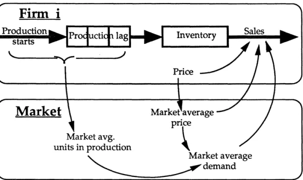
Figure 1 shows a schematic representation of the task, focusing on an individual firm and its interaction with the market. The market consists of K firms and a consumer sector. The market can be considered a regional industry where the level of activity and employment may influence aggregate demand in the region. The products of the indus-try have some limited degree of differentiation (the firm-demand elasticity is large but finite) but the market is otherwise close to the perfect-competition ideal.
Firms are operated by the subjects in the experiment while the demand side is simu-lated by computer. Substituting perfectly rational computer-simusimu-lated consumers for real people constitutes an afortiori assumption favoring the ability of markets to compensate for errors of the human producers.
Time is divided into discrete periods. At the beginning of each period, t, each firm, i, must decide how much production, y, to initiate and, in the posted-price condition, what price, p, to charge for its product this period. Firms make these decisions ex ante, i.e. without knowing demand for the period.
Each firm maintains a goods inventory, n, to accommodate fluctuations in demand. Inventories can be negative, corresponding to an order backlog. The inventory is decreased by sales, x, and increased by production. There may be a lag of 6 periods between the initiation of production, and the time it arrives in inventory. Thus, we have
(1) ni,t+l = ni,t + Yi,t6 xi,t
-Profits each period, v, are the difference between revenue and costs. Costs consist of production cost and inventory/backlog holding costs. Production costs are propor-tional to output. Holding costs are proporpropor-tional to the absolute value of inventory. Given unit production costs co and unit holding costs y, firm i's profit in period t is
(2) vi,t = Pi,txi,t - oxi,t -
Yni,tl.
Buyer utility is assumed to be a CES function of goods bought from individual firms with elasticity of substitution . Purchases of individual goods are combined into an aggregate good, X, according to
(3) Xt = K (xl,t )' + ... + XK -t( I)/) ( -1)
Defining an aggregate price index, P, such that total expenditures are equal to P-X according to
(4) 1 - )1/(1-£)
(4) Pt=
(
(Pl,t + ... + PK,t 1 ))(l)means utility-maximizing consumers, given total expenditures, generate demand x for firm i's product of
(5) xi,t = Xt (Pi,t/Pt)- .
Aggregate demand in period t, X, in turn depends on aggregate price, P. The elasticity of aggregate demand with respect to P is assumed to be a constant, p, around the competitive-equilibrium price p*. To ensure global robustness, demand becomes a linear function of price far from the competitive-equilibrium value (i.e. elasticity
D-4278 6
increases for rising prices and decreases for lower prices). Specifically, (6) Xt = Xt*f(Pt/p*); f(l) = 1; f'(.) < 0; f '(1) = -p;
(7) p* = /(- 1);
If the number of firms is very large, or if firms do not consider the effect of their own actions on aggregate quantities, then the competitive-equilibrium price equals p* and is independent of both X and P (Kampmann 1992).
Reference demand, X*, depends on total production activity, introducing a multiplier effect which can be interpreted as a consumption multiplier where income (production) drives demand. Thus X* consists of an autonomous demand component G, assumed to be constant, and a variable "multiplier" component proportional to market average production. Average production is the sum of current average production starts, Y and the average supply line, S, of production in process. Thus,
(8) Xt* = (1-a)G + a 1 -(Yt+St); 0< a < 1;
(9) Yt = (Yl,t + -.. + YK,t)/K; (10) St = (Yt- + .. + Yt-l).
The demand multiplier, a, and the production lag, 8, are both experimental treatment variables, as discussed above. In the "simple" case, xa=6=0. In the "complex" case, a=0.5 and 5=3 periods.
A marginal propensity to consume of 0.5 is lower than typical estimates for a closed economy. Simulation experiments shows that the system becomes prone to unrealisti-cally large fluctuations for high values of a. The lower value of a is thus an afortiori assumption: if the multiplier has strong effects when a=0.5, these are likely to be even larger for realistic values.
The ratio of unit inventory cost, y, to unit production cost, o, balances the need for III
positive profits while motivating subjects to control inventories. The chosen value of 0.5 was based on simulations and pilot experiments. Only 5 of 97 subjects suffered a
cumulative loss.
Finally, the firm and industry elasticities e=2.5 and g=.75. The industry elasticity is high compared to many typical goods industries (Hauthakker and Taylor 1970), another afortiori assumption favoring excellent performance in the market conditions. The unit production cost, co, and autonomous demand, G, are arbitrary as they determine only the scale of the variables; these were varied from market to market to discourage cross-market comparisons by subjects.
Hypotheses
Simulations and formal analysis (Kampmann 1992) demonstrate that if firms act according to the standard neoclassical assumptions of non-cooperation and rationality, the differences between the six conditions would be very small: In all cases, the markets should settle smoothly and rapidly (after a short initial learning period) to the non-cooperative equilibrium. If firms engage in strategic behavior the question of market convergence becomes more complicated. If all firms were committed to full collusion from the outset and never defected from the coalition, rational agents would quickly move the market to collusive equilibrium. Such a situation is unlikely; it is more plausi-ble that continuous attempts at achieving or defecting from cooperation would occur. Neoclassical economic theory offers no a priori reason to expect such attempts to follow a systematic pattern, and one would thus expect them to be essentially random, and the market should converge quickly to a stochastic stationary state.
If, however, individuals suffer from misperceptions of feedback such that their decision making heuristics do not account for the production lag or multiplier effect, significant differences in performance across conditions are predicted. In particular,
D-4278
* Complexity will decrease profits and stability in all three price regimes because sub-jects' mental models do not account well for delays and feedbacks. Oscillations are expected under complexity.
* The effects of complexity will be strongest under fixed prices, weaker under posted prices, and weakest under clearing prices. Fixed prices mean imbalances accumulate
in buffers, amplifying individual judgmental errors. Market-clearing prices eliminate inventory accumulation, automatically compensating for judgmental errors. Under posted prices subjects must adjust prices properly to clear out inventory imbalances, precisely the task non-market studies show to be problematic.
* Complexity will slow learning in all three price regimes because the excess variance makes inferences about causal structure and market dynamics more difficult.
* Collusion will be most evident in the simple (posted and clearing price) conditions and least evident in the complex posted-price condition, because the complex conditions are more demanding cognitively, reducing attention available for formulation of strategic behavior, and because excess variance complicates signalling and signal detection. Experimental Protocol
The market was implemented on a local-area-network of Macintosh computers which automatically administered and recorded all decisions and other events. Subjects sat at separate terminals, each person managing one firm in the market. Complete details of the protocol are provided in Kampmann (1992). Each market involved between three and six subjects (firms), with an average of four, shown in experimental economics to be generally enough to assure competitive conditions (Plott 1982, 1986).
Written instructions distributed as subjects arrived for the session described the objectives of the research and the market structure in general terms, subject decisions, and the basis for rewards. After reading the instructions and filling out a demographic
questionnaire, subjects played a practice session with three rounds of subject-determined production. The practice period provided an opportunity for subjects to learn the structure and parameters of the system. Subjects were free to ask questions before and during the trial. In each case, the system was initialized with production of 2/3 of the competitive-equilibrium level. The initial price was set to clear the market at the initial level of output.
At the beginning of each period, subjects made their production decision and, if applicable, set their price. After all decisions had been collected, the computers calcu-lated demand or prices for each firm, updated the information, and advanced time to the
beginning of the next period.
Subjects were free to take as long as they wished to make their decisions. Trials were halted after three hours or after subjects had played 50 time periods, whichever came first. The average length of each game was 44 time periods. The minimum was 35; the maximum of 50 was reached in 7 of the 24 markets. While subjects were not informed of the 50-period maximum, they were told that the game would be stopped within a fixed time. Thus, as was pointed out to the subjects, taking longer to deliberate would decrease the number of periods they could play, reducing their profits.
Subjects received a money award in proportion to their accumulated profits plus a minimum of $10 for participation. The average payout per subject was $34.80; 4 out of 97 subjects received only the minimum $10 payment while the maximum payment was $63, yielding per-hour compensation consonant with standards for experimental market
studies.
Subjects were primarily graduate and undergraduate students in economics and management at M.I.T. and Harvard University. The mean age was 24 years. Most had some formal education in economics and quantitative fields such as statistics or
opera-III
D-4278 10
tions research; many had taken advanced courses in these areas. To the extent possible, subject assignment was balanced with respect to education and affiliation. The experi-mental condition applied in any given session was determined randomly.
Throughout the game subjects had full local and aggregate information in the sense that they could observe past values of all variables characterizing their own firm, such as price, inventory, and production, and past values of the market average values of these variables. Such data are generally available in actual markets. Subjects did not, however, have full information about other firms. Firms also received some information about the distribution of individual prices (the highest and lowest price in the market). In the introductory description all the relevant structural relationships in the system, such as the factors affecting industry and individual-firm demand, were described, but subjects were not given numerical or mathematical details, other than an indication of the relative size of elasticities.
The information display showed relations between the stock of inventory and the flows of production and sales in diagrammatic form, with a summary spreadsheet of numerical values. Using pop-up menus subjects could access five tables showing the time-history of the market, three time-series graphs of market history, and three scatter plots, and could configure their own tables. To minimize possible information display effects the same display was maintained across all experimental conditions, with only the smallest modifications necessary to accommodate the different conditions.
Results
One compact measure of market behavior is the average profit earned by the partici-pant firms. Profits are the most relevant measure of subject performance since profits determined subject compensation. In the analysis below the first 10 periods have been excluded to minimize variations caused by initial learning and experimentation, and
profits are broken into two components: "gross profits" (profits before inventory costs), and "net profits" (after inventory costs).
Gross profits are primarily related to the price-output operating point of the market, i.e. a measure of the degree of collusion, whereas inventory costs are a function both of firm's production policy and the overall variation in prices and output, i.e. a measure of the degree of control. The relative importance of these two measures is inherently differ-ent in the three price regimes. Under fixed prices there is no possibility of collusion; in-ventory costs are the primary determinant of performance. Conversely, under clearing-prices inventory costs are eliminated; performance depends only on reaching the best price-output point. The posted-price regimes involve elements of both.
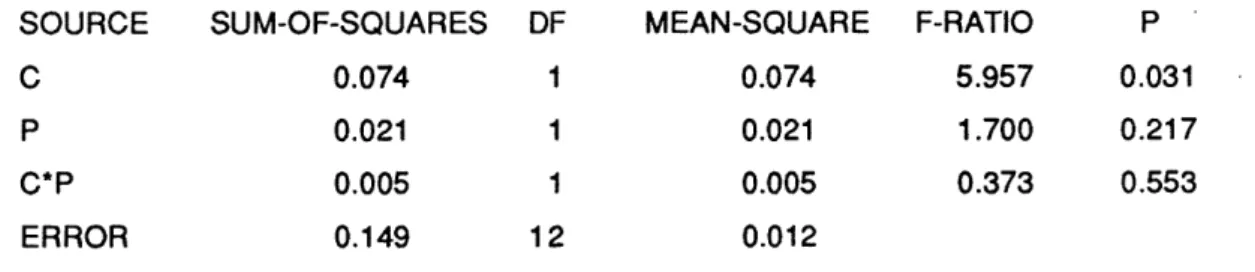
Table 1 reports analysis of variance of gross profits across experimental conditions. Gross profits have been normalized to an index which is 0 at the competitive profit level
and 1 at the collusive profit level. The index measures the average degree of collusion in the market. While the price regime has no significant effect, the effect of complexity is significant; on average, gross profits relative to optimal in the complex conditions are 10-15% lower than in the corresponding simple conditions, in some cases even falling below the competitive equilibrium level.
Table 2 repeats the analysis for inventory costs alone. The hypothesis of constant inventory costs in the non-clearing conditions is strongly rejected (p<0.1%).
Complexity has a very large effect on inventory costs - on average, inventory costs are about 13 times larger in the complex conditions. But there is also a strong interaction: the effect of complexity on inventory costs is much smaller in the posted-price than in the fixed-price regime.
Thus, the data do not support the rational expectations hypothesis. The data do con-firm many of the predictions of the behavioral hypotheses: Profits relative to optimal are
D-4278 12
lowered by the introduction of complexity in all three price regimes, sometimes dramati-cally. Most of the drop stems from higher inventory costs (except of course in the price-clearing conditions), but profits before inventory costs are lower as well. As a result, the effect of complexity on net profit is very large in the fixed-price and posted-price regimes, and smaller in the clearing-price regime. Finally, there is much greater variance in profits in the complex posted and fixed-price cases than in the other four conditions (The Bartlett test for homogeneity of group variances shows significant differences at p<O. 1%).
Market Dynamics and Convergence
Simulations show that if firms act rationally the experimental markets should con-verge in all six experimental conditions to a stochastic stationary state after about 10 time periods. The variation in market averages differs across conditions, but in all cases is
lower than the variance of any random errors in decision-making.
Figures 2-7 show the actual behavior of production and prices in each market for each of the experimental conditions. A quick glance reveals significant differences in the pattern of behavior across the conditions. The complex markets generally show larger and longer term variation in prices and quantities, and less tendency to converge to equilibrium, than the corresponding simple markets. There appear to be persistent cyclical movements in several of the complex markets.
In the simple condition with fixed prices (figure 2) production settles fairly quickly in the expected range. Apart from a few occasional departures from the equilibrium level, production is constant at its steady-state value. The task facing the decision maker here is a simple inventory control problem with a constant exogenous outflow. Previous experiments have shown, unsurprisingly, that humans perform quite well under such simple circumstances (Diehl 1992; MacKinnon and Wearing 1985).
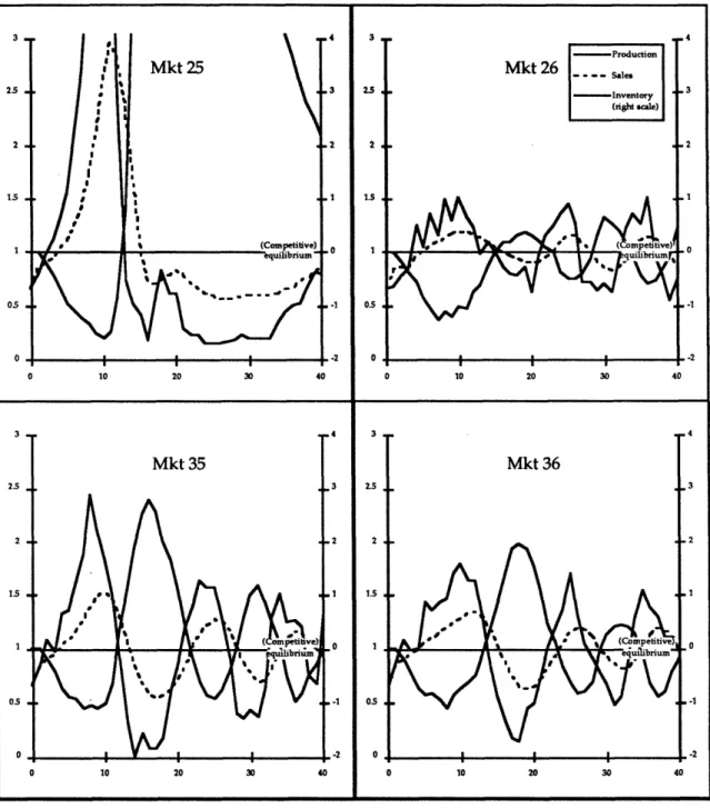
The variation in production is dramatically larger in the fixed-price complex condi-tion (Fig. 3). All markets show substantial cycles of "boom and bust". The initial increase in demand leads to inventory depletion before additional output can go through the supply line. In the face of rising demand and falling inventories, firms raise their production, leading to still higher demand, which in turn causes firms to raise production further. Because of the production delay and the continuous accumulation of inventory imbalances, firms have great difficulty catching up with demand. The upward spiral continues until higher production restores normal inventory levels, at which point all firms cut their production, leading to a decrease in demand and excessive unintended inventory accumulation. The result is a "recession" where production falls below equi-librium. The cycle in some markets is exceedingly large; in Market 25, output peaks at around four times the equilibrium value. None of the markets show any sign of being in equilibrium at the end of the trial.
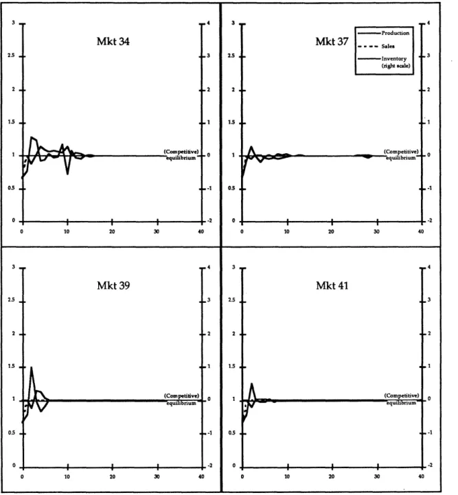
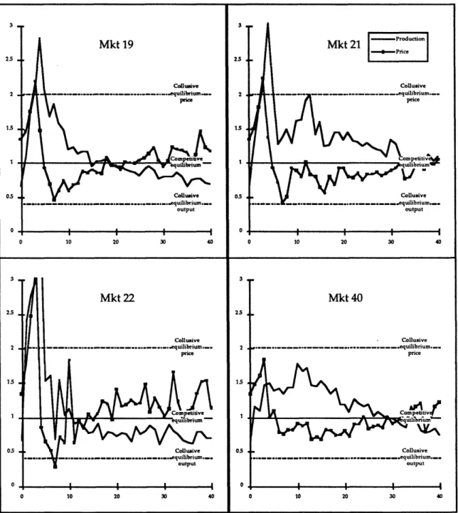
The markets with clearing prices also show marked differences between the simple and the complex condition. The markets in the simple clearing-price condition show no systematic pattern of behavior (Fig. 4). Some appear to settle in a range close to, or slightly above, the competitive price equilibrium, but with a fair amount of short-term fluctuation. Others show some longer-term fluctuation.
In contrast, the complex clearing-price markets all display a distinct "boom and bust" pattern of initial dramatic overshoot in production, followed by a gradual downward adjustment in output. Although the clearing-price complex condition shows a substantial initial boom and bust, the cycle is not sustained as it is in the corresponding fixed-price condition. A key structural difference between the fixed and clearing price regimes is the lack of cumulative effects of market imbalances in the latter. The market-clearing system effectively "forgets" past imbalances after they have gone through the pipeline delay,
D-4278 14
making it more forgiving of errors.
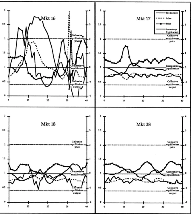
The posted-price markets also show effects of complexity on behavior. In the simple condition (Fig. 6), prices are relatively calm, and in three of the four, prices seem to be driven down towards the competitive level. In the fourth market (Mkt 32), firms change their prices little throughout most of the game. In all markets, inventories are kept closely in check and never depart substantially from the desired level.
The posted-price complex condition generally shows larger variance in prices and production compared to the simple case, although the variance differs from market to market (Fig. 7). One market (Mkt 16), exhibits dramatic, indeed expanding oscillations in prices and output. In two other markets, (Mkt 18 and Mkt 38), both prices and inven-tories and, in Mkt 18 also production, show a moderate but quite regular cycle. The last market (Mkt 17) shows relatively little variance in output or prices, except for a one-time peak in prices.
Spectral analysis confirmed what is evident from inspection of the results. While the spectra produced by rational agents will, after an initial learning period, be nearly white, the spectra of the experimental markets in the all complex conditions show the variance is concentrated in the low frequencies corresponding to the 10-20 period cycles or longer term movements evident in the figures.
Conclusion
The introduction of dynamic complexity results in significantly lower profits relative to optimal even in the presence of market institutions. Despite the introduction of finan-cial incentives and market institutions, the observed behavior shows strong evidence of misperceptions of feedback, although the consequences of these misperception are quite different in the different price regimes. The effects of poor mental models are most dramatic in the fixed-price regime, where subjects generated sustained cycles, replicating
previous non-market studies despite financial incentives for performance. In the clear-ing-price regime, automatic market clearing suppresses the accumulation of imbalances and thus makes the system much more forgiving of poor attention to delays and feed-back. In the posted-price regime, the possibility of using prices to control inventories makes the system potentially easier to handle. However, in three out of the four such markets, inventories and prices continue to oscillate throughout the trial: the cycle
involv-ing output and inventories in the fixed-price condition is replaced by one involvinvolv-ing prices and inventories in the posted-price condition. While much of the decrease in profits is the result of excessive inventory fluctuations, the introduction of complexity also made it more difficult for firms to find the price-output level that would maximize profits before inventory costs.
Plainly, models of dynamic decision making must include institutional features such as markets to capture the aggregate dynamics produced by the decision rules of the sub-jects. In particular, markets seem to moderate, but do not eliminate, the effects of
deci-sion-makers' misperceptions of feedback structure. However, the mere existence of markets does not imply that individual misperceptions of feedback are automatically ameliorated; models of economic dynamics must be grounded in empirical study of man-agerial decision making to capture the misperceptions of feedback which may produce systematically suboptimal dynamics even in the presence of well-functioning market institutions.
D-4278
References
Brehmer, B. (1990) Strategies in Real Time, Dynamic Decision Making, in Hogarth, R. (ed) Insights in Decision Making. Chicago: University of Chicago Press, 262-279.
Diehl, E. (1992). Effects of Feedback Structure on Dynamic Decision Making. PhD. Dissertation, MIT Sloan School of Management.
Funke, J. (1991). Solving Complex Problems: Exploration and Control of Complex Systems, in R. Sternberg and P. Frensch (eds.), Complex Problem Solving: Principles and Mechanisms. Hillsdale, NJ: Lawrence Erlbaum Associates.
Hauthakker, H. S., & Taylor, L. C. (1970). Consumer demand in the United States. Cambridge, MA: Harvard University Press.
Hogarth, R. M., & Reder, M. W. (1987). Rational Choice: The Contrast between Economics and Psychology. Chicago: Univ. of Chicago Press.
Kampmann, C. (1992). Feedback Complexity and Market Adjustment in Experimental Economics. PhD. Dissertation, MIT Sloan School of Management.
Kleinmuntz, D. (1985) "Cognitive Heuristics and feedback in a dynamic decision environment" Management Science 31: 680-702.
MacKinnon, A.J. and Wearing, A.J. (1985). "Systems Analysis and Dynamic Decision Making." Acta Psychologica. 58: 159-72.
Plott, C.R. (1982) "Industrial Organization Theory And Experimental Economics." Journal of Economic Literature 20: 1485-1527.
Plott, C.R. (1986). "Laboratory Experiments in Economics: The Implications of Posted-Price Institutions." Science. 232: 732-38.
Smith, V.L. (1986) Experimental methods in the political economy of exchange. Science 234: 167-235.
Smith, V.L. (1982) "Microeconomic Systems as an Experimental Science." American Economic Review 72: 923-55.
Smith, V., Suchanek, G., and A. Williams, 1988, Bubbles, Crashes, and Endogenous Expectations in Experimental Spot Asset Markets, Econometrica, 56(5), 1119-1152.
Sterman, J.D. (1989a). "Misperceptions of Feedback in Dynamic Decision Making." Organizational Behavior and Human Decision Processes. 43(3): 301-335.
Sterman, J.D. (1989b) "Modeling managerial behavior: Misperceptions of feedback in a dynamic decision-making experiment." Management Science 35: 321-339.
D-4278
Figure 1. Schematic representation of the experimental market III
Table 1. Analysis of variance of gross profits
Two-way analysis of variance of normalized average profits before inventory costs in each market, excluding the first 10 time periods, using price condition (P) and complexity (C) as factors. The normalization was
Index = Profits before inventory costs - Competitive equilibrium profits Collusive equilibrium profits
The fixed-price conditions were excluded since profits before inventory costs do not vary in the long run under fixed prices. N=16; Multiple-R2=.401.
SUM-OF-SQUARES 0.074 0.021 0.005 0.149 DF I 1 1 12 MEAN-SQUARE F-RATIO 0.074 5.957 0.021 1.700 0.005 0.373 0.012
Table 2. Analysis of variance of inventory costs
Two-way analysis of variance of the logarithm of the average inventory costs in each market, excluding the first 10 time periods, using price condition (P) and complexity (C) as factors. The clearing-price conditions have been excluded: inventories are identically zero in these cases. N=16; Multiple-R2=.798.
SUM-OF-SQUARES 81.308 13.070 33.654 32.368 DF MEAN-SQUARE 1 81.308 1 13.070 1 33.654 12 2.697 SOURCE C P C*P ERROR P 0.031 0.217 0.553 SOURCE C P C*P ERROR F-RATIO 30.144 4.846 12.477 P 0.000 0.048 0.004
Mkt 34 (Competitive) equilibrium ' 10 I 30 20 30 -4 -3 O1 -o -1 I 40 Mkt 39
I
(Competitive) pit-R~~~~~ 4V ~equilibrium -I I I 10 20 30 .4 .3 .2 .1 2 40 3 2.5 2 1.5 1 0.5 0 3 2.5 2 1.5 1 0.5 0 I I 10 20 0 10 20 30 3O 4 3 0 -2 40 4 -3 .1 0 -1 -2 30 40Figure 2 Observed behavior of market averages: fixed-price simple condition
The figure shows market-average production, sales, and inventory for each of the four markets in the condition, relative to the equilibrium output level. Inventory is shown on the right-hand scale. D-4278 3 253 2. 20 1.5 roucio Production Mkt 37
.
Ses Inventory (riht sale) A -- _ -- (Competitive) equilibrium'rV
1 0.5 0 0 3 254 2 15 1 0.5 o0 Mkt 41 - - equilibrium I I I 0 ! I ..-0-- ri- re isL
dE lee !I I -1 I 0A
nI (Competitive) i I0 10
I
20 30 0 10 20 30 3 2.5 2 1.5 05 0.5 10 20 30 40 25 2 1.5 05I
0 10 20 30 40Figure 3 Observed behavior of market averages: fixed-price complex condition
The figure shows market-average production, sales, and inventory for each of the four
markets in the condition, relative to the equilibrium output level. Inventory is shown on the
right-hand scale.
3 25 2 I 05 0 3 2 0 0 -1 -2 3 2.5 2 15 1 05 0 - -|111 0 10 20 30 40 Mkt 31 Collusive __.__.__e,,__,.,_,_.._. rie price Collusive ... .--.,. e ., .. , quilibrium... output
1I
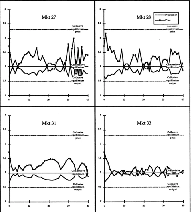
i I I i 0 3 25 2 1.5 0.5 0 3 2.5 2 1.5 0 0.5 0 0 10 20 30 40 Mkt 33 Collusive ..---. ___.. ... _.. .u .equilibrium.. price t _<~~opetitive ~~~~~~~ output I I Ii 0 10 20 30 40Figure 4 Observed behavior of market averages: clearing-price simple condition
Figure shows market average production, sales, and price relative to competitive equilibrium. Also shown are the collusive-equilibrium price and output. Note the differences in the
qualitative pattern of behavior between the simple and complex conditions.
D-4278 22 3 25 2 1 05 0 3 25 2 1.5 1 05 0 10 20 30 40 q P~~~~~~~~~~~~~~~~~~~~~~~~~~~~~~~~~~~~~~~~~~~~~~~~~~~~~~~~~~~~~~~~~~~~~~~~~ MI' I ! I - I lI -- = i - I --·--·I I
0 10 20 30 40 Mkt 22 Collusive __,....___...._ .._ .equrnaDrwm._. price l I l Competilive I ou~~~~~~~~~.tput I I I 10 20 30 40 3 25 2 IS 03 0 3 25 2 15 1 05 0 0 10 20 30 40 0 10 20 30 40
Figure 5 Observed behavior of market averages: clearing-price complex condition
Figure shows market average production, sales, and price relative to competitive equilibrium.
Also shown are the collusive-equilibrium price and output.
3 25 2 1.5 1 05 0
' I
3 25 2 15 05 0 0tl
]IT!
I
'1t
r
-rAl
lMkt 23 Collusive I'_...__.._. ... ___...__._.l i .equilibrium_..oe price T'~~~'>mput iive Collusive output -4 -3 .2 0 10 20 30 40 3 2 1 0 -1 -2 10 20 30 40 3 25 2 15 1 05 0 3 25s 2 15 1 05 0 0 10 20 30 40 0 10 20 30 .4 .3 .2 ,0 -2 40
Fgure 6 Observed behavior of market averages: posted-price simple condition
The figures show market-average production, sales, price and inventory for each of the four markets, relative to the equilibrium output level. Inventory is shown on the right-hand scale. The collusive equilibrium is also shown.
D-4278 24 3 2.5 2 1.5 1 0.5 0 0 3 2.5 2 1.5 1 0.5 0 Mkt 32 Collusive _..__.__._._,, .____...,.___.__equrlm price _LL- JCIL ~mpettv _ ~~~~~~~~~Co mpet i iv e ... Ii i% Collusive . __.__ ... __ ._ ____ .. _ __equilibrium output
!
L
I· I I -Z I 1 1 1 111 I 1 I . I 4 L I I I 00 10 20 30 40 0 10 20 30 40 3 2.5 2 is15 05 O 25 2 1.5 I 0.5 0 0 10 20 30 * 40 0 10 20 30 40
Figure 7. Observed behavior of market averages: posted-price complex condition
The figures show market-average production, sales, price and inventory for each of the four
markets, relative to the equilibrium output level. Inventory is shown on the right-hand scale.
The collusive equilibrium is also shown.
3 25 2 15 1 05 0 3 25 2 15 I 05 0 t ,