HAL Id: hal-01587535
https://hal.archives-ouvertes.fr/hal-01587535
Submitted on 27 Oct 2020
HAL is a multi-disciplinary open access
archive for the deposit and dissemination of
sci-entific research documents, whether they are
pub-lished or not. The documents may come from
teaching and research institutions in France or
abroad, or from public or private research centers.
L’archive ouverte pluridisciplinaire HAL, est
destinée au dépôt et à la diffusion de documents
scientifiques de niveau recherche, publiés ou non,
émanant des établissements d’enseignement et de
recherche français ou étrangers, des laboratoires
publics ou privés.
Stijn Hantson, Almut Arneth, Sandy P. Harrison, Douglas I. Kelley, I. Colin
Prentice, Sam S. Rabin, Sally Archibald, Florent Mouillot, Steve R. Arnold,
Paulo Artaxo, et al.
To cite this version:
Stijn Hantson, Almut Arneth, Sandy P. Harrison, Douglas I. Kelley, I. Colin Prentice, et al.. The
status and challenge of global fire modelling. Biogeosciences, European Geosciences Union, 2016, 13
(11), pp.3359 - 3375. �10.5194/bg-13-3359-2016�. �hal-01587535�
www.biogeosciences.net/13/3359/2016/ doi:10.5194/bg-13-3359-2016
© Author(s) 2016. CC Attribution 3.0 License.
The status and challenge of global fire modelling
Stijn Hantson1, Almut Arneth1, Sandy P. Harrison2,3, Douglas I. Kelley2,3, I. Colin Prentice3,4, Sam S. Rabin5, Sally Archibald6,7, Florent Mouillot8, Steve R. Arnold9, Paulo Artaxo10, Dominique Bachelet11,12, Philippe Ciais13, Matthew Forrest14, Pierre Friedlingstein15, Thomas Hickler14,16, Jed O. Kaplan17, Silvia Kloster18,
Wolfgang Knorr19, Gitta Lasslop18, Fang Li20, Stephane Mangeon21, Joe R. Melton22, Andrea Meyn23, Stephen Sitch24, Allan Spessa25,26, Guido R. van der Werf27, Apostolos Voulgarakis21, and Chao Yue13
1Karlsruhe Institute of Technology, Institute of Meteorology and Climate research, Atmospheric Environmental
Research, 82467 Garmisch-Partenkirchen, Germany
2School of Archaeology, Geography and Environmental Sciences (SAGES), University of Reading, Reading, UK 3School of Biological Sciences, Macquarie University, North Ryde, NSW 2109, Australia
4AXA Chair of Biosphere and Climate Impacts, Grand Challenges in Ecosystem and the Environment, Department of Life
Sciences and Grantham Institute, Climate Change and the Environment, Imperial College London, Silwood Park Campus, Buckhurst Road, Ascot SL5 7PY, UK
5Department of Ecology & Evolutionary Biology, Princeton University, Princeton, NJ, USA
6School of Animal, Plant and Environmental Sciences, University of the Witwatersrand, Johannesburg 2050,
South Africa
7Natural Resources and the Environment, CSIR, P.O. Box 395, Pretoria, 0001, South Africa
8UMR5175 CEFE, CNRS/Université de Montpellier/Université Paul-Valéry Montpellier/EPHE/IRD,
1919 route de Mende, 34293 Montpellier CEDEX 5, France
9Institute for Climate and Atmospheric Science, School of Earth & Environment, University of Leeds, Leeds, UK 10Institute of Physics, University of São Paulo, Rua do Matão, Travessa R, 187, CEP05508-090, São Paulo, S.P., Brazil 11Biological and Ecological Engineering, Oregon State University, Corvallis, OR 97331, USA
12Conservation Biology Institute, 136 SW Washington Ave., Suite 202, Corvallis, OR 97333, USA
13Laboratoire des Sciences du Climat et de l’Environnement, LSCE/IPSL, CEA-CNRS-UVSQ, Université Paris-Saclay,
91198 Gif-sur-Yvette, France
14Senckenberg Biodiversity and Climate Research Institute (BiK-F), Senckenberganlage 25,
60325 Frankfurt am Main, Germany
15College of Engineering Mathematics and Physical Sciences, University of Exeter, Exeter, UK
16Institute of Physical Geography, Goethe University, Altenhöferallee 1, 60438 Frankfurt am Main, Germany 17Institute of Earth Surface Dynamics, University of Lausanne, 1015 Lausanne, Switzerland
18Max Planck Institute for Meteorology, Bundesstraße 53, 20164 Hamburg, Germany
19Department of Physical Geography and Ecosystem Science, Lund University, 22362 Lund, Sweden 20International Center for Climate and Environmental Sciences, Institute of Atmospheric Physics,
Chinese Academy of Sciences, Beijing, China
21Department of Physics, Imperial College London, London, UK
22Climate Research Division, Environment Canada, Victoria, BC, V8W 2Y2, Canada
23Karlsruhe Institute of Technology, Atmosphere and Climate Programme, 76344 Eggenstein-Leopoldshafen, Germany 24College of Life and Environmental Sciences, University of Exeter, Exeter EX4 4RJ, UK
25Department of Environment, Earth and Ecosystems, Open University, Milton Keynes, UK 26Department Atmospheric Chemistry, Max Planck Institute for Chemistry, Mainz, Germany 27Faculty of Earth and Life Sciences, VU University Amsterdam, De Boelelaan 1085, 1081HV,
Amsterdam, the Netherlands
Received: 16 January 2016 – Published in Biogeosciences Discuss.: 25 January 2016 Revised: 4 May 2016 – Accepted: 23 May 2016 – Published: 9 June 2016
Abstract. Biomass burning impacts vegetation dynamics, biogeochemical cycling, atmospheric chemistry, and climate, with sometimes deleterious socio-economic impacts. Under future climate projections it is often expected that the risk of wildfires will increase. Our ability to predict the magni-tude and geographic pattern of future fire impacts rests on our ability to model fire regimes, using either well-founded empirical relationships or process-based models with good predictive skill. While a large variety of models exist today, it is still unclear which type of model or degree of complex-ity is required to model fire adequately at regional to global scales. This is the central question underpinning the creation of the Fire Model Intercomparison Project (FireMIP), an in-ternational initiative to compare and evaluate existing global fire models against benchmark data sets for present-day and historical conditions. In this paper we review how fires have been represented in fire-enabled dynamic global vegetation models (DGVMs) and give an overview of the current state of the art in fire-regime modelling. We indicate which chal-lenges still remain in global fire modelling and stress the need for a comprehensive model evaluation and outline what lessons may be learned from FireMIP.
1 Introduction
Each year, about 4 % of the global vegetated area is burnt (Giglio et al., 2013; Randerson et al., 2012). Fire is the most important type of disturbance and as such is a key driver of vegetation dynamics (Bond et al., 2005), both in terms of succession and in maintaining fire-adapted ecosystems (Fur-ley et al., 2008; Staver et al., 2011; Hirota et al., 2011; Rogers et al., 2015). Fires play an essential role in ecosystem func-tioning, species diversity, plant community structure and car-bon storage. The impact fire has on the ecosystem depends on the local fire regime, which includes a range of impor-tant characteristics such as fire frequency, intensity, season-ality, etc. Fire is also important through its effect on radiative forcing, biogeochemical cycling, and biogeophysical effects (Bond-Lamberty et al., 2007; Bowman et al., 2009; Ward et al., 2012; Yue et al., 2016).
Global carbon dioxide emissions from biomass burning are estimated to be about 2 PgC (P = 1015)per year, of which approximately 0.6 PgC yr−1comes from tropical deforesta-tion and peat fires (van der Werf et al., 2010). This is equiva-lent to ca. 25 % of those from fossil fuel combustion (Boden et al., 2013; Ciais et al., 2014), although in the absence of climate and/or land-use change, nearly all of these emissions are taken up during vegetation regrowth after fire. Together,
fire significantly decreases the net carbon gain of global ter-restrial ecosystems by 1.0 Pg C yr−1averaged across the 20th century (Li et al., 2014). Fire emissions are also an important driver of inter-annual variability in the atmospheric growth rate of CO2(van der Werf et al., 2004, 2010; Prentice et al.,
2011; Guerlet et al., 2013) and a significant contribution to the atmospheric budgets of CH4, CO, N2O and many other
atmospheric constituents. As a source of aerosol (including black carbon) and ozone precursors (Voulgarakis and Field, 2015), emissions from fires contribute directly and indirectly to radiative forcing (Myhre et al., 2013; Ward et al., 2012), reducing net shortwave radiation at the surface and warming the lower atmosphere, thus affecting regional temperature, clouds, and precipitation (Tosca et al., 2010, 2014; Ten Ho-eve et al., 2012; Boucher et al., 2014) and regional- to large-scale atmospheric circulation patterns (Tosca et al., 2013; Zhang et al., 2009). Through their impacts on ozone, and as a source of CO and volatile organic compounds, fires also affect the atmospheric abundance of the OH radical, which determines the atmospheric lifetime of the greenhouse gas methane (Bousquet et al., 2006). In addition, ozone produced from fires is directly harmful to plants, reducing photosyn-thesis (Pacifico et al., 2015) and fire-emitted aerosol can shift the balance between diffuse and direct radiation (Mercado et al., 2009; Cirino et al., 2014). Deposition of fire-produced N (Chen et al., 2010) and P aerosols (Wang et al., 2015) can enhance productivity in nutrient-limited ecosystems.
Fire also has direct effects on human society: more than 5 million people globally were affected by the 300 major fire events in the past 30 years, with economic losses of more than USD 50 billion (EM-DAT; http://www.emdat.be, Guha-Sapir et al., 2015). Air quality is regionally affected by the occurrence of fire due to increases in aerosol and ozone that are harmful to human health. At a regional scale, hospitaliza-tions and human deaths increase in major fire years (Marlier et al., 2013). The degradation of air quality caused by fire is estimated to result in 260 000 to 600 000 premature deaths globally each year (Johnston et al., 2012).
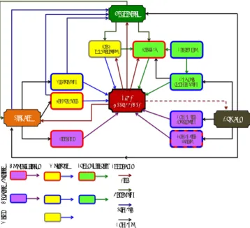
Given that fire impacts so many aspects of the earth sys-tem, there is considerable concern about what might happen to fire regimes in response to projected climate changes in the 21st century. However, as the IPCC Fifth Assessment Report (AR5) made clear, “there is low agreement on whether cli-mate change will cause fires to become more or less frequent in individual locations” (Settele et al., 2014). This is in large part due to the complexity of the interactions and feedbacks between vegetation, people, fire and other elements of the earth system (Fig. 1), which is not well represented in cur-rent Earth system models. Fire, vegetation, and climate are intimately linked: changes in climate drive changes in fire
FIRE
OCCURRENCE
Lightning Human Ĩire Ɛtarts
Human fire suppression Land use fragmentation Humans Fuel load Fuel characteristics Vegetation Climate Precipitation Temperature No of ignitions P osit iv e Neg ativ e
Moisture Fuel continuity
Mix ed Fire Feedbacks Vegetation Climate Humans Herbivores
Figure 1. Summary of the interactions between the controls on fire occurrence on coarse scales. Green-, yellow-, and purple-filled boxes represent controls influencing fuel, moisture, and ignition, re-spectively. Red-outlined boxes indicates positive influence on fire, while blue indicates a negative influence and brown a mixed re-sponse. Brown arrows indicate interactions between people and other controls, and dark green arrows represent interactions between vegetation and other controls; dark blue arrows represent feedback from climate, black arrows show direct effects, and red arrows show feedback from fire. The arrow from fragmentation to fuel load indi-cates its effect on fuel continuity.
as well as changes in vegetation that provides the fuels for fire, and in return fire alters vegetation structure and com-position, with feedbacks to climate through changing sur-face albedo, ecosystem properties, and transpiration and as a source of CO2, other trace gases, and aerosols, altering
at-mospheric composition and chemistry (Ward et al., 2012). Human activities strongly affect fire regimes (Bowman et al., 2011; Archibald et al., 2013) due to the use of fire for land management, while the use of fire as a tool in the deforesta-tion process is still occurring in the tropics (e.g. Morton et al., 2008). Humans may also suppress fire directly or indi-rectly through land-use change (Bistinas et al., 2014; Knorr et al., 2014; Andela and van der Werf, 2014). Grazing her-bivores (the densities of which are also often controlled by humans) can also decrease fire occurrence by reducing fuel loads (Pachzelt et al., 2015).
Statistical models have been used to examine the poten-tial trajectory of changes in fire during the 21st century (e.g. Moritz et al., 2012; Settele et al., 2014). Such models es-sentially assess the possibility of fire occurring given cli-mate conditions and fuel availability (fire risk or fire dan-ger) based on modern-day relationships between climate, fuel, and some aspects of the fire regime such as burnt area. However, changes in fire risk/danger will not necessarily be
closely coupled to changes in fire regime in the future given the direct impacts of CO2 on water-use efficiency,
produc-tivity, vegetation density, and ultimately vegetation compo-sition and distribution. This limits the utility of statistically based models for the investigation of feedbacks to climate through fire-driven changes of land-surface properties, veg-etation structure or atmospheric composition – feedbacks which have the potential to exacerbate or ameliorate the ef-fects of future climate change on ecosystems as well as in-fluence the security and well-being of people.
In contrast to statistical models, fire-enabled dynamic global vegetation models (DGVMs) and terrestrial ecosys-tem models (TEMs) can address some of the feedbacks be-tween fire and vegetation. Coupling fire-enabled DGVMs with climate and atmospheric chemistry models in an Earth system model (ESM) framework allows the feedbacks be-tween fire and climate to be examined. There has been a rapid development of fire-enabled DGVMs in the past two decades with many DGVMs currently including fire as a standard process. Four out of the 15 carbon-cycle mod-els in the MsTMIP (Multi-scale Synthesis and Terrestrial Model) intercomparison project (Huntzinger et al., 2016), 5 out of 10 carbon-cycle models in TRENDY (Trends in net land-atmosphere carbon exchange over the period 1980– 2010; http://dgvm.ceh.ac.uk/), and 9 ESMs in CMIP5 (fifth phase of the Coupled Model Intercomparison Project; https:// pcmdi.llnl.gov/search/esgf-llnl/) provide fire-related outputs. The complexity of the fire component of these models varies enormously – from simple empirically based schemes for predicting burnt area to models that explicitly simulate the process of ignition and fire spread to models that incorporate fire adaptations and their impact on the vegetation response to fire. However, to date there has been no systematic com-parison and evaluation of these models, and thus there is no consensus about the level of complexity required to model fire and fire-related feedbacks realistically.
The Fire Model Intercomparison Project (FireMIP), ini-tiated in 2014, is a collaboration between fire modelling groups worldwide to address this issue. Modelling groups participating in FireMIP will run a set of common exper-iments to examine fire under present-day and past climate scenarios, and will conduct systematic data–model compar-isons and diagnosis of these simulations with the aim of pro-viding an assessment of the reliability of future projections of changes in fire occurrence and characteristics. There has been no previous attempt to compare fire models across a suite of standardized experiments (model–model compari-son) or to systematically evaluate model performance using a wide range of different benchmarks (data–model compari-son).
The main objective of the current manuscript is to present an overview of the current state-of-the-art fire-enabled DGVMs as a background to the FireMIP initiative. We first present an overview of the current state of knowledge about the drivers of global fire occurrence. We indicate how these
have been treated over time in different fire models and de-scribe the variety in state-of-the-art fire-enabled DGVMs. Fi-nally, we give a short overview of the plans for FireMIP and the overall philosophy behind the model benchmarking and evaluation.
2 The controls on fire
Fire is driven by complex interactions between climate, veg-etation and people (Fig. 1), which vary in time and space. On meteorological timescales (i.e. minutes to days) and limited spatial scales (i.e. metres to kilometres), atmospheric circula-tion patterns and moisture adveccircula-tion determine the locacircula-tion, incidence, and intensity of lightning storms that produce fire ignitions. Weather and vegetation state also determine sur-face wind speeds and vapour-pressure gradients, and hence the rates of fuel drying, which in turn affect the probability of combustion as well as fire spread. However, topography also affects the spread of fire: fire fronts travel faster uphill because of upward convection of heat, while rivers, lakes, and rocky outcrops can act as natural barriers to fire fronts.
On longer timescales (i.e. seasons to years) and larger spa-tial scales (i.e. regional to continental), temperature and pre-cipitation exert a major effect on fire because these climate variables influence net primary productivity (NPP), vegeta-tion type and the abundance, composivegeta-tion, moisture content, and structure of fuels. Burnt area tends to be lowest in very wet or very dry environments, and highest where the water balance is intermediate between these two states. Related to this, burnt area is greatest at intermediate levels of NPP and decreases with both increases and decreases in productivity. These unimodal patterns along precipitation or productivity gradients emerge due to the interaction between moisture availability and productivity: dry areas have low NPP, which limits fuel availability and continuity, while NPP and hence fuel loads are high in wet areas but the available fuel is gen-erally too wet to burn. Temperature exerts an influence on the rate of fuel drying in addition to its influence on NPP. Season-ality in water availability also plays a role here: for any given total amount of precipitation, fire is more prevalent in sea-sonal climates because fuel accumulates rapidly during the wet season and subsequently dries out. While the vegetation and fuel exert an important control on fire occurrence, fire impacts vegetation distribution and structure, causing impor-tant vegetation–fire feedbacks. At a local scale, fires create spatial heterogeneity in fuel amount, influencing subsequent fire spread and limiting fire growth.
While natural factors are important drivers of global fire occurrence, human influences are also pervasive. People start fires, either accidentally or with a purpose, for example for forest clearance, agricultural waste burning, pasture manage-ment, or fire management. People can also affect fire regimes through land conversion from less flammable (forest) vege-tation to more flammable (grassy) vegevege-tation. The
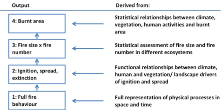
introduc-4: Burnt area
2: Ignition, spread, extinction 3: Fire size x fire number
Statistical relationships between climate, vegetation, human activities and burnt area
Statistical assessment of fire size and fire number in different ecosystems Functional relationships between climate, human and vegetation/ landscape drivers of ignition and spread
Full representation of physical processes in space and time
Output Derived from:
1: Full fire behaviour
Figure 2. Summary of the levels of model complexity required to derive different aspects of global fire regimes. Outputs from mod-els functioning at level 1 can be used to derive higher-level outputs, but it is not possible to work backwards (i.e. empirical relationships between burnt area and environmental drivers will not allow for as-sessment of changes in fire number and fire size). Currently there are fire routines in global DGVMs that represent all of these levels of complexity (see Table 1).
tion of flammable invasive species is another cause of chang-ing fire occurrence. Changes in land use can also reduce fuel loads through crop harvesting, grazing, and forestry. Hu-man activities lead to fragmentation of natural vegetation, which affects fire spread, and fires are also actively sup-pressed. There is a unimodal statistical relationship between burnt area and population density. At extremely low popu-lation densities, increasing popupopu-lation is associated with an increase in fire numbers and burnt area. At high population densities, increasing population is associated with a decrease in burnt area. However, in general, when climate and vegeta-tion factors are accounted for, there is a monotonic negative relationship between burnt area and human population – i.e. burnt area decreases with increasing human presence (Bisti-nas et al., 2014; Knorr et al., 2014). The unimodal statisti-cal relationship of burnt area with population density (and other socio-economic variables such as gross domestic prod-uct (GDP) that are linked to population density) results from the co-variance of population density with vegetation pro-duction and moisture (Bistinas et al., 2014). Low population densities are found in very dry or cold climates where vegeta-tion productivity and fuel loads are also minimal. High pop-ulation densities are (generally) found in moist environments with high vegetation productivity but where moist conditions limit fire spread.
3 History and current status of global fire modelling While not explicitly representing fire occurrence, early veg-etation models often included a generic treatment of distur-bance on plant mortality. There are two basic types of fire models that are applied in global vegetation models (Fig. 2): (a) top-down “empirical models” based on statistical rela-tionships between key variables (climate, population
den-sity) and some aspect of the fire regime, usually burnt area, and (b) bottom-up “process-based models” which represent small-scale fire dynamics (i.e. by simulating individual fires), before scaling up to calculate fire metrics for an entire grid cell. The boundaries between these two types are not rigid, however, and some models combine features of both. Fire models have developed in parallel, and there have been dif-ferences as well as some overlap between the approaches taken by different models to representing key processes. Our goal here is therefore not to describe every single fire model in detail, but rather to outline the major approaches to key processes and in particular to focus on models when they in-troduced fundamentally new approaches.
3.1 Empirical global fire models
The absence of global-scale fire information before remotely sensed burnt-area products became available was a common challenge to the development of fire models and hindered testing and parameterization of empirical algorithms. The GLOBal FIRe Model (Glob-FIRM; Thonicke et al., 2001) was the first global fire model, based on the notion that once there is sufficient combustible material burnt area depends on the length of the fire season. The fire season length is cal-culated as the summed daily “probability of fire” which is a function of the fuel moisture (approximated by the moisture in the upper soil layer), and the moisture of extinction. The functions relating moisture content, fire season length, and burnt area were calibrated using site-based observations. In addition, Glob-FIRM has a threshold value of 200 gC m−2 to represent the point at which fuel becomes discontinuous and the probability of fire occurring is zero. Glob-FIRM was initially developed for inclusion in the Lund–Potsdam–Jena (LPJ) DGVM (Sitch et al., 2003), but has since been cou-pled into several other DGVMs (with some modifications), including the Common Land Model (Dai et al., 2003), the Community Land Model (CLM; Levis et al., 2004), the OR-ganizing Carbon and Hydrology In Dynamic EcosystEms (ORCHIDEE; Krinner et al., 2005), the Lund–Potsdam– Jena General Ecosystem Simulator (LPJ-GUESS; Smith et al., 2001), the Biosphere Energy-Transfer Hydrology model (BETHY; Kaminski et al., 2013), and the Institute of At-mospheric Physics, Russian Academy of Sciences Climate Model (IAP RAS CM; Eliseev et al., 2014). A simple fire model with a similar structure to Glob-FIRM, has also been included in the Jena Scheme for Biosphere-Atmosphere Cou-pling in Hamburg (JSBACH) global vegetation model (Reick et al., 2013).
Some empirical models include human impacts on fire oc-currence. Typically, algorithms are used that link fire proba-bility/frequency to both an estimate of lightning ignition and to human population density. Pechony and Shindell (2009) proposed an algorithm whereby the number of fires increases with population, levelling off at intermediate population den-sities and then decreasing to mimic fire suppression under
high population densities (Table 1). The simulated number of fire counts is then converted into burnt area using an “ex-pected fire size” scaling algorithm (Pechony and Shindell, 2009). The human ignition and suppression relationships de-scribed by Pechony and Shindell (2009) have been adopted by several other, both empirical and process-based fire– vegetation models (Table 1). INteractive Fires and Emissions algoRithm for Natural envirOnments (INFERNO; Mangeon et al., 2016) is an integrated fire and emission model for JULES and HadGEM (the UK Met Office’s coupled climate model) based on the Pechony and Shindell (2009) approach, but water vapour pressure deficit is used as one of the main indicators of flammability in the model, while an inverse ex-ponential relationship is used to relate flammability to soil moisture. In an alternative approach, Knorr et al. (2014) used a combination of weather information (to account for fire risk) with remotely sensed data of vegetation properties that are linked to fire-spread and information on global popula-tion density to derive burnt area in a multiple-regression ap-proach. This model has been coupled to LPJ-GUESS DGVM (Knorr et al., 2016).
3.2 Process-based global fire models
MC-FIRE (Lenihan et al., 1998; Lenihan and Bachelet, 2015) was the first attempt to simulate fire via an explicit, process-based, rate-of-spread (RoS) model. MC-FIRE calcu-lates whether a fire occurs in a grid cell on a given day, based on whether the grid cell is experiencing drought conditions and that the “probability of ignition and spread”, as jointly determined by the moisture of the fine fuel class and the sim-ulated rate of spread, is greater than 50 %. The rate of spread is calculated based on equations by Rothermel (1972), which represent the energy flux from a flaming front based on fuel size, moisture, and compaction. Canopy fires are initiated us-ing the van Wagner (1993) equations. All of the grid cell is assumed to burn if a fire occurs – i.e. the original MC-FIRE was designed to simulate large, intense fires. Later work in-troduced functions to suppress area burnt by low-intensity and/or slow-moving fires (Rogers et al., 2011). MC-FIRE in-spired the development of several process-based, RoS-based models, and many fire-enabled DGVMs still use a similar basic framework (Table 1).
The Regional Fire Model (Reg-FIRM: Venevsky et al., 2002) introduced a new approach in fire modelling by sim-ulating burnt area as the product of number of fires and av-erage fire size. Reg-FIRM assumes a constant global light-ning ignition rate, and includes human ignitions depending on population density. It then uses the Nesterov index, an empirical relationship between weather and fire, to determine the fraction of ignitions that start fires. Every fire occurring during a given day in a given grid cell is assumed to have the same properties and thus be the same size. Reg-FIRM uses a simplified form of the Rothermel (1972) equations to cal-culate rate of spread; these effectively depend only on wind
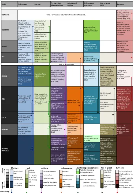
Table 1. Representation of fire processes in fire-enabled DGVMs. The intensity of the colour represents the complexity of the description of the process. Shades of grey describe the complexity of the model as a whole: light grey is the simplest and black the most complex. Blue represents the complexity of description of moisture control on fire susceptibility ranging from simple statistical relationships/fire danger indices (FDIs) of fuel as a whole (light blue) to description of moisture in multiple fuel size classes to fully modelled or specifically chosen FDIs for specific fuel moisture (dark blue). Green represents the complexity of fuel controlled fire susceptibility: simple masking at a specified fuel threshold (light green); fuel structure effects on ignition probability and rate of spread; and complex modelling of fuel bulk density (dark green). Purple shows complexity of natural ignition schemes: no specified/assumed ignitions (white); constant ignition source (light purple); simple relationship with fuel moisture; prescribed ignitions – normally through lightning climatology inputs; prescribed lightning with additional scaling for, for example, latitude-dependent cloud-to-ground lightning (CG); daily distributed lightning via a weather generator; and with additional complex ignition simulation (dark purple). Orange represents anthropogenic ignitions: none (white); constant background ignition source (light orange); ignitions varying based on human population density based on a “human ignition potential” (HIP) and/or gross domestic product (GDP); and inclusion of additional, complex human ignition schemes such as pre-historic human behaviour (dark orange). Cyan and lime green represent inclusion of human ignitions suppression and agriculture: none (white); constant suppression (light cyan); increasing suppression with population (medium cyan); simple agricultural masking of fire (light lime green); fuel load manipulation from agriculture (lime green); and a mix of agricultural and ignition suppression (dark cyan). Italic text under “human ignitions” and “human suppression” denotes models where the combined influence of human ignitions and suppression result in a unimodal description of fire relative to population density. Brown shows complexity of the calculation of fire sizes, typically through a rate-of-spread model (RoS): none (white); simplified RoS model to obtain fire properties (light brown); simplified RoS to model individual fires; full Rothermel RoS; and multiple RoS models (dark brown). Red shows complexity of the calculation of the overall burnt area: the entire cell is affected by fire (light red); constant scaling of the number of fires to burnt area depending on vegetation type; scaling based on moisture and fuel type; entirety of a sub-cell affected; and scaling of number of fires by fire size calculated by RoS model. Arrows demonstrate the exchange of components between models. Arrows start in the model containing the original process description.
Model Fuel moisture Fuel load Fire starts from lightning ignitions Anthropogenic ignitions Anthropogenic suppression Rate of spread (ROS) Burnt area
CASA/GFED None. Fire translated to burnt area from satellite fire counts.
Proportional to no. of fires, with more burnt area to fire in sparse vegetation (van der Werf, 2003)
GLOBFIRM
Moisture of extinction, above which fire does not occur (Thonicke et al. 2001)
Discontinuity fuel load threshold, below which fire does not occur (Thonicke et al. 2001)
Suppression from reduced fuel from grazing (Krinner et al. 2005
Increases exponentially with annual (Thonicke et al. 2001) or monthly (Krinner et. al. 2005) summed fire occurrence. Increased fire occurrence with (Thonicke et al. 2001)
Reduced fuel from grazing (Krinner et. al. 2005)
SIMFIRE
Maximum possible burnt area a function of FDI (Knorr et al. 2014)
Maximum possible fire as a function of fAPAR as proxy fuel load (Knorr et al. 2014)
Increases exponentially with population (Knorr et al. 2014; Knorr et al. 2016)
Multiplication of maximum fire functions for fuel, moisture & suppression (Knorr et al. 2014).
P&S
Function of VPD (proxy for ambient atmospheric conditions) (Pechony & Shindell, 2009) Fire scaled by vegetation density based on LAI (Pechony & Shindell, 2009)
Observed lightning flash count, scaled for cloud-to-ground (CG) ratio (Pechony & Shindell, 2009) Increases with population (Pechony & Shindell, 2009) MC-FIRE
Calculated from fuel size classes and live fuel component
(Lenihan et al. 1998). Size ratios effects RoS (Rothermel 1972)
1000hr hour fuel content drops below threshold and rate of spread is above a threshold (Lenihan et al. 1998)
Capped burnt area for low intensity or slow spread rate fires in populated areas (Rogers et al. 2011)
Fire behaviour scaled by fuel load and moisture-based fire danger index (FDI) based rate of spread for ground (Rothermal 1972; Lenihan et al. 1998) and crown (Van Wanger, 1993) fires
Entire grid cell affected by fire during fire occurrence (Lenihan et al. 1998)
Affects fire start (Lenihan et al. 1998) and RoS (Rothermel 1972)
CTEM
Represented by soil moisture (Arora & Boer 2005; Melton & Arora 2016)
Linear increase fire occurrence between discontinuity and saturated fuel thresholds (Arora & Boer 2005)
Probability of fire occurrence a multiple of probabilities from fuel, moisture & ignitions (Arora & Boer 2005).
Maximum of 1 fire per sub-grid cell unit. Overall burnt area in grid cell is multiplication of probability of fire by number of units by average fire size per unit (Arora & Boer 2005; Melton & Arora 2016)
Deforestation fire (Kloster et al. 2012)
No. of days fire burnt suppressed at higher population density (Melton & Arora 2016)
No FDI (Arora & Boer 2005)
Affected by differing fuel types (Arora & Boer 2005)
Latitude-dependent CG scaling for lightning (Kloster et al. 2012)
Li et al. Represented by soil moisture &relative humidity (Li et al. 2012)
Ignitions & limitation from fuel and moisture (Li et al., 2012)
Deforestation & degradation fires in tropical closed forests (Li et al. 2013) Suppression increases with GDP (Li et al. 2013) REGFIRM Number of fires instead of probability of fire (Venesky et al. 2002) ‘Human ignition potential’(HPI) (Venesky et al. 2002)
Variable wind speed affects rate of spread and fire oval shape (Venesky et al. 2002)
multiplied by average area burnt per fire (Venesky et al. 2002)
Fire occurrence based FDI (Venesky et al. 2002)
SPITFIRE/ LPX/Lmfire
HIP varying with development (Thonicke et al. 2010) Cropland fire masking (Thonicke et al. 2010) CG distributed between wet and dry lightning (Prentice et al. 2011)
Multi-day fires (Pfeiffer et al. 2013) Different RoS for different vegetation type (Pfeiffer et al. 2013) Additional ignition suppression term (Thonicke et al. 2010) “Storm days” (Kelley
et al. 2014)
Different human-fire relation for hunter-gatherers, pastoralists and farmers (Pfeiffer et al. 2013)
Terrain impediment to spread (Pfeiffer et al. 2013) Inter-annual lightning from atmospheric conditions (Pfeiffer et al. 2013) Explicit cropland fragmentation algorithm (Pfeiffer et al. 2013) Reduced rate of spread at high wind speeds (Lasslop et al. 2014)
Moisture Fuel Ignitions Anthropogenic Anthropogenic suppression Rate of spread
Simple Compl ex Empirical/FDI base Multiple fuel moisture types + multiple FDI Masking threshold Size classes/ ROS Complex Constant/assumed Moisture based Lightning scaling + complex weather Constant + additional ignition algorithm Agricultural masking
Varies with pop. density + agricultural masking Simplified Rothermel Full Rothermel Multiple spread types Relationship + weather generator
from pop. density Constant suppression
+ complex masking Fuel manipulation Fire function of fuel load deforestation fires
Uses RoS fire properties
Burnt area
Simple scaling of no. fires Empirically related to fuel and moisture Entire sub-cell Average burnt area multiplied by no. fires Entire cell affected decreasing moisture
for
Rate-of-spread models
Fire only occurs when
from moisture-
Socio-economic
Number of fires
speed, fuel moisture (as approximated by near-surface soil moisture), and PFT-dependent fuel bulk density. Fire dura-tion is determined stochastically from an exponential distri-bution with a mean of 24 h to account for the fact that less frequent large fires account for a disproportionate amount of the total area burnt. The RoS equations are used to estimate the burnt surface by approximating the shape of the fire as an ellipse, as suggested by van Wagner (1969).
The fire module in the Canadian Terrestrial Ecosystem Model (CTEM: Arora and Boer, 2005; Melton and Arora, 2016) uses a variant of the Reg-FIRM scheme where the pre-defined FDI approach is replaced by an explicit calcu-lation of susceptibility, which is the product of the probabili-ties associated with fuel, moisture, and ignition constraints on fire (Table 1). Ignitions are either caused by lightning, the incidence of which varies spatially, or anthropogenic. Anthropogenic ignition is constant in CTEMv1 (Arora and Boer, 2005) but varies with population density in CTEMv2 (Melton and Arora, 2016). As in Reg-FIRM, fire duration is determined in such a way as to incorporate the disproportion-ate area burnt by long-lasting fires, but CTEM does this de-terministically rather than stochastically. CTEM includes fire suppression via a “fire extinguishing” probability to account for suppression by natural and man-made barriers, as well as deliberate human suppression of fires. The fire model devel-opment in CLM (Kloster et al., 2010; Li et al., 2012, 2013) is based on the CTEM work but introduced anthropogenic igni-tions and suppression on fire occurrence as funcigni-tions of pop-ulation density. Li et al. (2013) also set anthropogenic igni-tions and suppression as funcigni-tions of gross domestic produc-tion (GDP) and introduced human suppression on fire spread. The SPread and InTensity of FIRE (SPITFIRE) model (Ta-ble 1; Thonicke et al., 2010) is a RoS-based fire model de-veloped within the Lund–Potsdam–Jena (LPJ) DGVM. It is a further development of the Reg-FIRM approach, but SPIT-FIRE uses a more complete set of physical representations to calculate both rate of spread and fire intensity. However, maximum fire duration is limited to 4 h. Anthropogenic ig-nitions are a function of population density as in REGFirm, although the function is regionally tuned in SPITFIRE. Fire is excluded from agricultural areas, but SPITFIRE effectively includes human fire suppression on other lands because hu-man ignitions first increase and then decrease with increasing population density. The SPITFIRE model has been imple-mented with modifications in other DGVMs, including OR-CHIDEE (Yue et al., 2014), JSBACH (Lasslop et al., 2014), LPJ-GUESS (Lehsten et al., 2009), and CLM(ED) (Fisher et al., 2015).
Some fire models based on SPITFIRE, such as the Land surface Processes and eXchanges model (LPX; Prentice et al., 2011; Kelley et al., 2014) and the Lausanne–Mainz fire model (LMfire; Pfeiffer et al., 2013), have introduced further changes into the ignitions scheme. Natural ignition rates in both models are derived from a monthly lightning climatol-ogy, as in SPITFIRE, but LPX preferentially allocates
light-ning to days with precipitation (which precludes burlight-ning) such that only a realistic number of days have ignition events. Similarly to LPX, LMfire limits lightning strikes to rain days, and also estimates interannual variability in lightning igni-tions by scaling a lightning climatology using long-term time series of convective available potential energy (CAPE) pro-duced by atmosphere models. LMfire further reduces light-ning ignitions based on the fraction of land already burnt, since lightning tends to strike repeatedly in the same parts of the landscape while being rare in others. LPX and LM-fire also modified the treatment of anthropogenic burning relative to the original SPITFIRE. LMfire specified that the number of anthropogenic ignitions differs amongst liveli-hoods by distinguishing human populations into three basic categories: hunter-gatherers, pastoralists, and farmers. Each of these populations has different behaviour with respect to burning based on assumptions regarding land management goals. LPX, on the other hand, does not include human igni-tions on the grounds that the supposed positive relaigni-tionship of population density to fire activity is an artefact, as dis-cussed above. Finally, LMfire accounts for the constraint on fire spread imposed by fragmentation of the burnable land-scape by human land use (as well as topography), while indi-vidual fires are allowed to burn across multiple days, and fires occurring simultaneously within the same grid cell can effec-tively coalesce as they grow larger. Like LMfire, the HES-FIRE model (Le Page et al., 2015) also focuses on the con-straints on fire spread – using landscape fragmentation (due to human activities, topography, or past fire events) to deter-mine the probability of extinction of a fire that is ignited.
Schemes to simulate anthropogenic fire associated explic-itly with land-use change have also been developed. Kloster et al. (2010) include burning associated with land-use change by assuming that some fraction of cleared biomass is burnt. This fraction depends on the probability of fire as medi-ated by moisture, such that the combusted fraction is low in wet regions (e.g. northern Europe) and high in dry regions (e.g. central Africa). Li et al. (2013) proposed an alternative scheme to model fires caused by deforestation in the tropical closed forests, in which fires depended on deforestation rate and weather/climate conditions and were allowed to spread beyond land-type conversion regions when weather/climate conditions are favourable. When the scheme was used in their global fire model, fires due to human and lightning ignitions described in Li et al. (2012) were not used in the tropical closed forests. Li et al. (2013) also include cropland man-agement fires, prescribing seasonal timing based on satellite observations but allowing the amount of burning to depend on the amount of post-harvest waste, population density, and gross domestic product, and fires in peatlands, depending on a prescribed area fraction of peatland distribution, climate, and area fraction of soil exposed to air. The Li et al. scheme has been the basis for the fire development in the Dynamic Land Ecosystem Model (DLEM; Yang et al., 2015). A
sim-ple representation of peat fires is also present in the IAP RAS CM (Eliseev et al., 2014).
3.3 Modelling the impact of fire on vegetation and emissions
The impact of fire on vegetation operates through combus-tion of available fuel, plant mortality, and triggering of post-fire regeneration. There is more similarity in the treatment of fire impacts between models than many other aspects of fire. Glob-FIRM assumes that all the aboveground lit-ter/biomass is burnt, while subsequent models assume that only a fraction of the available fuel is burnt. In CTEM, the completeness of combustion varies by fuel class and PFT (Arora and Boer, 2005), while models such as MC-FIRE and SPITFIRE include a dynamic scheme for completeness of combustion which depends on fire characteristics and the moisture content of each fuel class (Thonicke et al., 2010; Lenihan et al., 1998).
Post-fire vegetation mortality is generally represented in a relatively simple way in fire-enabled DGVMs (Table 2). Glob-FIRM, CTEM, Reg-FIRM, and the models described by Li et al. (2012) and Kloster et al. (2010) use PFT-specific parameters for fractional mortality. MC-FIRE has a more ex-plicit treatment of mortality, in which fire intensity and res-idence time influence tree mortality from ground fires via crown scorching and cambial damage. Canopy height rela-tive to flame height (which is a function of fire intensity) determines the extent of crown scorching. Bark thickness, which scales with tree diameter, protects against damage to the trunk, such that thicker-barked trees have more chance of surviving a fire of a given residence time. LPJ-SPITFIRE uses a similar approach except that bark thickness scales with tree diameter, which, together with canopy height, de-pends on woody biomass. LMfire includes a simple repre-sentation of size cohorts within each PFT, with the bark thickness scalar being defined explicitly for each size cohort. In contrast, gap-based vegetation–fire models such as LPJ-GUESS-SPITFIRE/SIMFIRE (Lehsten et al., 2009; Knorr et al., 2016) and CLM(ED) (Fisher et al., 2015) explicitly sim-ulate size cohorts within patches characterized by differen-tial fire-disturbance histories. LPX-Mv1 (Kelley et al., 2014) incorporates an adaptive bark thickness scheme, in which a range of bark thicknesses is defined for each PFT. Since thinner-barked trees are more likely to be killed by fire, the distribution of bark thickness within a population changes in response to fire frequency and intensity.
LPX-Mv1 (Kelley et al., 2014) is the only model to date to incorporate an explicit fire-triggered regeneration process, which it does through creating resprouting variants of the temperate broad-leaved and tropical broad-leaved tree PFTs. Resprouting trees are penalized by having low recruitment rates into gaps caused by fire and other disturbances. How-ever, resprouting is only one part of the syndrome of vege-tation responses to fire which include, for example, obligate
seeding, serotiny, and clonal reproduction (e.g. Pausas and Keeley, 2014).
4 Objective and organization of FireMIP
Existing fire models have very different levels of complex-ity, with respect to both different aspects of the fire regime within a single model and different families of models. It is not clear what level of complexity is appropriate to simulate fire regimes globally. Given the increasing use of fire-enabled DGVMs to project the impacts of future climate changes on fire regimes and estimate fire-related climate feedbacks (e.g. Knorr et al., 2016; Kelley and Harrison, 2014; Kloster et al., 2012; Pechony and Shindell, 2010), it is important to address this question.
Coordinated experiments using identical forcings allow comparisons focusing on differences in performance driven by structural differences between models. The baseline FireMIP simulation will use prescribed climate, CO2,
light-ning, population density, and land-use forcings from 1700 through 2013. Examination of the simulated vegetation and fire during the 20th century will allow differences between models to be quantified, and any systematic differences be-tween types of models or with model complexity to be iden-tified.
However, a single experiment of this type is unlikely to be sufficient to diagnose which processes cause the differences between models. Various approaches can be used for this purpose, including sensitivity experiments and parameter-substitution techniques. Similarly, the effect of model com-plexity can be examined by switching off specific processes. In FireMIP, experiments will be performed to study the im-pact of lightning, pre-industrial burnt area, CO2, nitrogen,
and fire itself between different models.
Many model intercomparison projects have shown that model predictions may show reasonably good agreement for the recent period but then diverge strongly when forced with a projected future climate scenario (e.g. Flato et al., 2014; Friedlingstein et al., 2014; Harrison et al., 2015). “Out-of-sample” evaluation is one way of identifying whether good performance under modern conditions is due to the concate-nation of process tuning. Within FireMIP, we will use simu-lations of fire regimes for different climate conditions in the past (i.e. outside the observational era used for parameteriza-tion and/or parameter tuning) as a further way of evaluating model performance and the causes of model–model differ-ences.
5 Benchmarking and evaluation in FireMIP
Evaluation is integral to the development of models. Most studies describing vegetation-model development provide some assessment of the model’s predictive ability by compar-ison with observations (e.g. Sitch et al., 2003; Woodward and
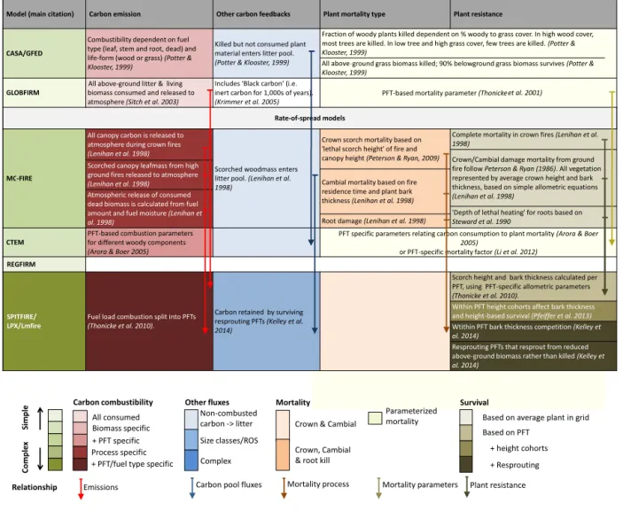
Table 2. Representation of the impacts of fire in fire-enabled DGVMs. Intensity of colour indicates the complexity of the description of the component. Green indicates complexity of the representation of fire impacts. Red describes the complexity of the description of atmospheric fluxes from fire: flux is equivalent to all consumed biomass (light red); consumption based on biomass-specific combustion parameters; inclusion of PFT combustion parameters; process-based; and biomass/PFT parameterized process-based (dark red). Blue represents the complexity of carbon fluxes to other carbon pools: no additional fluxes (white); non-combusted dead carbon flux (light blue); carbon fluxes based on fire spread properties; and fire-adapted vegetation carbon retention (dark blue). Orange represents complexity of simulated mortality processes: parameterized morality (yellow); mortality from crown and cambial damage (light orange); and additional root damage mortality (dark orange). Brown represents complexity of plant adaptation to fire when mortality processes are included: mortality based on a grid cell’s “average plant” properties of fire-resistant traits (light brown); PFT-based average traits; inclusion and height cohorts; and inclusion of dynamic/complex adaptations such as resprouting (RS) (dark brown). Arrows demonstrate the exchange of components between models, starting in the model containing the original description.
Model (main citation) Carbon emission Other carbon feedbacks Plant mortality type Plant resistance
CASA/GFED
Combustibility dependent on fuel type (leaf, stem and root, dead) and life-form (wood or grass) (Potter & Klooster, 1999)
Killed but not consumed plant material enters litter pool. (Potter & Klooster, 1999)
Fraction of woody plants killed dependent on % woody to grass cover. In high wood cover, Klooster, 1999)
All above-Klooster, 1999) GLOBFIRM biomass consumed and released to
atmosphere (Sitch et al. 2003)
Includes ‘Black carbon’ (i.e. (Krimmer et al. 2005)
PFT-based mortality parameter (Thonicke
Rate-of-spread models
MC-FIRE
All canopy carbon is released to atmosphere during crown fires (Lenihan et al. 1998)
Scorched woodmass enters litter pool. (Lenihan et al. 1998)
Crown scorch mortality based on 'lethal scorch height' of fire and canopy height (Peterson & Ryan, 2009)
Complete mortality in crown fires (Lenihan et al. 1998)
Crown/Cambial damage mortality from ground fire follow Peterson & Ryan (1986). All vegetation represented by average crown height and bark thickness, based on simple allometric equations (Lenihan et al. 1998)
Scorched canopy leafmass from high ground fires released to atmosphere
(Lenihan et al. 1998) Cambial mortality based on fire
residence time and plant bark thickness (Lenihan et al. 1998) Atmospheric release of consumed
dead biomass is calculated from fuel amount and fuel moisture (Lenihan et al. 1998)
'Depth of lethal heating' for roots based on Steward et al. 1990
Root damage (Lenihan et al. 1998) CTEM
PFT-based combustion parameters for different woody components (Arora & Boer 2005)
PFT specific parameters relating carbon consumption to plant mortality (Arora & Boer 2005)
or PFT-specific mortality factor (Li et al. 2012) REGFIRM
SPITFIRE/ LPX/Lmfire
Fuel load combustion split into PFTs (Thonicke et al. 2010).
Carbon retained by surviving resprouting PFTs (Kelley et al. 2014)
Scorch height and bark thickness calculated per PFT, using PFT-specific allometric parameters (Thonicke et al. 2010).
Within PFT height cohorts affect bark thickness and height-based survival (Pfeiffer et al. 2013) Wtithin PFT bark thickness competition (Kelley et al. 2014)
Resprouting PFTs that resprout from reduced above-ground biomass rather than killed (Kelley et al. 2014)
Simple
Compl
ex
All consumed
Carbon combustibility Other fluxes
Non-combusted carbon -> litter Size classes/ROS Complex
Mortality
Crown & Cambial Crown, Cambial & root kill
Parameterized mortality
Relationship Emissions Carbon pool fluxes Mortality process
Survival
Based on average plant in grid
Plant resistance Biomass specific
+ PFT specific Process specific + PFT/fuel type specific
Based on PFT + height cohorts + Resprouting Mortality parameters
inert carbon for 1,000s of years). All above-ground litter & living
most trees are killed. In low tree and high grass cover, few trees are killed. (Potter & ground grass biomass killed; 90% belowground grass biomass survives (Potter &
et al. 2001)
Lomas, 2004; Prentice et al., 2007). However, these compar-isons often focus on the novel aspects of the model and are largely based on qualitative measures of agreement such as map comparison (e.g. Gerten et al., 2004; Arora and Boer, 2005; Thonicke et al., 2010; Prentice et al., 2011). How-ever, they often do not track improvements or degradations in overall model performance caused by these new devel-opments. The concept of model benchmarking, promoted by the International Land Model Benchmarking Project (IL-AMB: http://www.ilamb.org), is based on the idea of a com-prehensive evaluation of multiple aspects of model
perfor-mance against a standard set of targets using quantitative metrics. Model benchmarking has multiple functions, includ-ing (a) showinclud-ing whether processes are represented correctly, (b) discriminating between models and determining which perform better for specific processes, and (c) making sure that improvements in one part of a model do not compro-mise performance in another (Randerson et al., 2009; Luo et al., 2012; Kelley et al., 2013). Since fire affects many inter-related aspects of ecosystem dynamics and the Earth system, with many interactions being non-linear, the last of which is particularly important for fire modelling.
Kelley et al. (2013) have proposed the most comprehen-sive vegetation-model benchmarking system to date. This system provides a quantitative evaluation of multiple sim-ulated vegetation properties, including primary production, seasonal net ecosystem production, vegetation cover, com-position and height, fire regime, and runoff. The benchmarks are derived from remotely sensed gridded data sets with global coverage and site-based observations with sufficient coverage to sample a range of biomes on each continent. Data sets derived using a modelling approach that involves calculation of vegetation properties from the same driving variables as the models to be benchmarked are explicitly ex-cluded. The target data sets in the Kelley et al. (2013) scheme allow comparisons of annual average conditions and seasonal and inter-annual variability. They also allow the impact of spatial and temporal biases in means and variability to be separately assessed. Specifically designed metrics quantify model performance for each process and are compared to scores based on the temporal or spatial mean value of the observations and to both a “mean” and “random” model pro-duced by bootstrap resampling of the observations. The Kel-ley et al. (2013) scheme will be used for model evaluation and benchmarking in FireMIP. It has been shown that spatial resolution has no significant impact on the metric scores for any of the targets (Harrison and Kelley, unpublished data); nevertheless, model outputs will be interpolated to the 0.5◦ common grid of the data sets for convenience.
The Kelley et al. (2013) scheme does not address key as-pects of the coupled vegetation–fire system including the amount of above-ground biomass and/or carbon, fuel load, soil moisture, fuel moisture, the number of fire starts, fire in-tensity, the amount of biomass consumed in individual fires, and fire-related emissions. Global data sets describing some of these properties are now available, and will be included in the FireMIP benchmarking scheme. These data sets in-clude above-ground biomass derived from vegetation opti-cal depth (Liu et al., 2015) as well as ICESAT-GLAS lidar data (Saatchi et al., 2011), the European Space Agency Cli-mate Change Initiative Soil Moisture product (Dorigo et al., 2010), the Global Fire Assimilation System biomass-burning fuel consumption product, fire radiative power, and biomass-burning emissions (Kaiser et al., 2012), and fuel consump-tion (van Leeuwen et al., 2014). The selecconsump-tion of new data sets is partly opportunistic, but it reflects the need to evalu-ate all aspects of the coupled vegetation–fire system as well as the importance of using data sets that are derived inde-pendently of any vegetation model that uses the same driv-ing variables as the coupled vegetation–fire models bedriv-ing benchmarked. The goal is to provide a sufficient and robust benchmarking scheme for evaluation of fire while ensuring that other aspects of the vegetation model can also be evalu-ated, and to this end new data sets will be incorporated into the FireMIP benchmarking scheme as they become available during the project.
The FireMIP benchmarking system will represent a sub-stantial step forward in model evaluation. Nevertheless, there are a number of issues that will need to be addressed as the project develops, specifically how to deal with the existence of multiple data sets for the same variable, how to exploit process understanding in model evaluation, and how to en-sure that models which are tuned for modern conditions can respond to large changes in forcing. The answers to these questions remain unclear, but here we provide insights into the nature of the problem and suggest some potential ways forward.
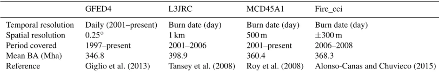
The selection of target data sets, in particular how to deal with differences between products and uncertainties, is an important issue in benchmarking. There are, for example, multiple burnt-area products (e.g. GFED4, L3JRC, MCD45, and Fire_cci: see Table 3). In addition to the fact that all of these products systematically underestimate burnt area be-cause of difficulties in detecting small fires (Randerson et al., 2012; Padilla et al., 2015), they differ from one another. Al-though all four products show a similar spatial pattern with more burnt area in the tropical savannas and less in temper-ate and boreal regions, L3JRC and MCD45 have a higher to-tal burnt area than MERIS or GFED4 (Table 3). Differences between products are lower (though still substantial) in the tropical savannas than elsewhere; extra-tropical regions are the major source of uncertainty between products (Fig. 3a). The same is true for interannual variability (Fig. 3b), where differences between products are higher in regions where to-tal burnt area is low. Most products show an increase in burnt area between 2001 and 2007 in extra-tropical regions, but there are disagreements even for the sign of regional changes (Fig. 3c). These types of uncertainties, which are also char-acteristic of other data sets, need to be taken into account in model benchmarking – either by focusing on regions or fea-tures which are robust across multiple products or by explic-itly incorporating data uncertainties in the benchmark scores (see e.g. Hargreaves et al., 2013).
Process analyses can provide an alternative approach to model evaluation. The idea here is to identify relationships between key aspects of a system and potential drivers, based on analysis of observations, and then to determine whether the model reproduces these relationships (see e.g. Lasslop et al., 2014; Li et al., 2014). It is important to use techniques that isolate the independent role of each potential driving variable because relationships between assumed drivers are not necessarily causally related to the response. Bistinas et al. (2014) showed, for example, that burnt area increases as NPP increases and decreases as fuel moisture increases. Given that increasing precipitation increases both NPP and fuel moisture this results in a peak in fire at intermediate levels of NPP and precipitation. Population density is also strongly influenced by NPP (i.e. the capacity of the land to provide ecosystem services) and thus the apparent unimodal relationship between burnt area and population density (see e.g. Aldersley et al., 2011) is an artefact of the relationship
Table 3. Overview of the burnt-area (BA) products used for the intercomparison and their characteristics.
GFED4 L3JRC MCD45A1 Fire_cci
Temporal resolution Daily (2001–present) Burn date (day) Burn date (day) Burn date (day)
Spatial resolution 0.25◦ 1 km 500 m ±300 m
Period covered 1997–present 2001–2006 2001–present 2006–2008
Mean BA (Mha) 346.8 398.9 360.4 368.3
Reference Giglio et al. (2013) Tansey et al. (2008) Roy et al. (2008) Alonso-Canas and Chuvieco (2015)
Figure 3. Coefficient of variation (%) characterizing (a) inter-product variability in mean burnt area; (b) the inter-inter-product vari-ability of the interannual varivari-ability in burnt area; and (c) the inter-product variability of the slope of temporal trends (2001–2007). Plots (a) and (b) are based on all four burnt-area products (GFED4, MCD45, L3JRC, Fire_cci) whereas plot (c) is based on three prod-ucts and does not include the MERIS data because it is currently only available for 3 years, see Table 3.
between population density and NPP. However, when appro-priate techniques are used to isolate causal relationships, the ability to reproduce these relationships establishes that the model is simulating the correct response for the right rea-son. Thus, process evaluation goes a step beyond benchmark-ing and assesses the realism of model behaviour rather than simply model response, a very necessary step in establishing confidence in the ability of a model to perform well under substantially different conditions from present.
One goal of FireMIP is to develop modelling capacity to predict the trajectory of fire-regime changes in response to projected future climate and land-use changes. It has been repeatedly shown that vegetation and carbon-cycle models that reproduce modern conditions equally well produce very different responses to future climate change (e.g. Sitch et al., 2008; Friedlingstein et al., 2014). The interval for which we have direct observations is short and does not encompass the range of climate variability expected for the next cen-tury. Benchmarking using modern observations does not pro-vide an assessment of whether model performance is likely to be realistic under radically different climate conditions. The climate-modelling community use records of the pre-observational era to assess how well models simulate cli-mates significantly different from the present (Braconnot et al., 2012; Flato et al., 2014; Harrison et al., 2014, 2015; Schmidt et al., 2014). FireMIP will extend this approach to the evaluation of fire-enabled vegetation models, building on the work of Brücher et al. (2014). Many data sources pro-vide information about past fire regimes. Charcoal records from lake and mire sediments provide information about lo-cal changes in fire regimes through time (Power et al., 2010) and have been used to document spatially coherent changes in biomass burnt (Daniau et al., 2012; Marlon et al., 2008, 2013). Hemispherically integrated records of vegetation and fire changes can be obtained from records of trace gases (e.g. carbon monoxide) and markers of terrestrial productivity and biomass burning (e.g. carbonyl sulfide, ammonium ion, black carbon, levoglucosan, vanillic acid) in polar ice cores (e.g. Wang et al., 2010, 2012; Kawamura et al., 2012; Asaf et al., 2013; Petrenko et al., 2013; Zennaro et al., 2014). Both hemi-spherically integrated and spatially explicit records of past changes in fire will be used for model evaluation in FireMIP.
6 Conclusions and next steps
Fire has profound impacts on many aspects of the Earth system. We therefore need to be able to predict how fire regimes will change in the future. Projections based on statis-tical relationships are not adequate for projections of longer-term changes in fire regimes because they neglect potential changes in the interactions between climate, vegetation and fire. While mechanistic modelling of the coupled vegetation– fire system should provide a way forward, it is still necessary
to demonstrate that they are sufficiently mature to provide reliable projections. This is a major goal of the FireMIP ini-tiative.
There has been enormous progress in global fire modelling over the past 10–15 years. Knowledge about the drivers of fire has improved, and understanding of fire feedbacks to cli-mate and the response of vegetation is improving. Global fire models have developed from simulating burnt area only to representing most of the key aspects of the fire regime. How-ever, there are large and to some extent arbitrary differences in the representation of key processes in process-based fire models and little is known about the consequences for model performance. While the development of fire models has been towards increasing complexity, it is still not clear whether a global fire model needs to represent ignition, spread, and ex-tinction explicitly or whether it would be sufficient to just represent the emergent properties of these processes (burnt area, or fire size, season, intensity, and fire number) in mod-els with fewer uncertain parameters. The answer to this ques-tion may depend on whether the goal is to characterize the role of fire in the climate system or to understand the interac-tion between fire and vegetainterac-tion. Burnt area and biomass are the key outputs needed to quantify fire frequency and car-bon, aerosol, and reactive trace gas emissions and changes in albedo required by climate and/or atmospheric chemistry models. Empirical models may be adequate to estimate such changes. Other aspects of the fire regime are important fac-tors with respect to the vegetation response to fire and thus may require a more explicit simulation of, for example, fire intensity and crown fires. FireMIP will address these issues by systematically evaluating the performance of models that use different approaches and have different levels of com-plexity in the treatment of processes in order to establish whether there are aspects of simulating modern and/or fu-ture fire regimes that require complex models. Systematic evaluation will also help guide future development of in-dividual models and potentially the further development of vegetation–fire models in general.
FireMIP is a non-funded initiative of the fire-modelling community. Participation in the development of benchmark-ing data sets and analytical tools, as well as in the runnbenchmark-ing and analysis of the model experiments, is open to all fire sci-entists. We hope this will maximize exchange of informa-tion between modelling groups and facilitate rapid progress in this area of science.
Data availability
The international disaster database can be ac-cessed at http://www.emdat.be/. The Firecci grid-ded burnt-area product can be downloaded from https://www.geogra.uah.es/esa/grid.php, the L3JRC global burnt-area product can be downloaded from http://forobs.jrc.ec.europa.eu/products/burnt_areas_L3JRC/ GlobalBurntAreas2000-2007.php, the MCD45 global
burnt-area products can be downloaded from http://modis-fire. umd.edu/pages/BurnedArea.php?target=Download and the GFED4 gridded burnt-area data can be downloaded from http://www.globalfiredata.org/data.html.
Acknowledgements. Stijn Hantson and Almut Arneth acknowledge support by the EU FP7 projects BACCHUS (grant agreement no. 603445) and LUC4C (grant agreement no. 603542). This work was supported, in part, by the German Federal Ministry of Education and Research (BMBF), through the Helmholtz Association and its research programme ATMO, and the HGF Impulse and Networking fund. The MC-FIRE model development was supported by the global change research programmes of the Biological Resources Division of the US Geological Survey (CA 12681901,112-), the US Department of Energy (LWT-6212306509), the US Forest Service (PNW96–5I0 9 -2-CA), and funds from the Joint Fire Science Program. I. Colin Prentice is supported by the AXA Research Fund under the Chair Programme in Biosphere and Climate Impacts, part of the Imperial College initiative Grand Challenges in Ecosystems and the Environment. Fang Li was funded by the National Natural Science Founda-tion (grant agreement no. 41475099 and no. 2010CB951801). Jed O. Kaplan was supported by the European Research Council (COEVOLVE 313797). Sam S. Rabin was funded by the National Science Foundation Graduate Research Fellowship, as well as by the Carbon Mitigation Initiative. Allan Spessa acknowledges fund-ing support provided by the Open University Research Investment Fellowship scheme. FireMIP is a non-funded community initiative and participation is open to all. For more information, contact Stijn Hantson ([email protected]).
The article processing charges for this open-access publication were covered by a Research
Centre of the Helmholtz Association.
Edited by: A. V. Eliseev
References
Aldersley, A., Murray, S. J., and Cornell, S. E.: Global and regional analysis of climate and human drivers of wild-fire, Science of The Total Environment, 409, 3472–3481, doi:10.1016/j.scitotenv.2011.05.032, 2011.
Alonso-Canas, I. and Chuvieco, E.: Global burned area mapping from Envisat-Meris and Modis active fire data, Remote Sens. En-viron., 163, 140–152, doi:10.1016/j.rse.2015.03.011, 2015. Andela, N. and van der Werf, G. R.: Recent trends in African fires
driven by cropland expansion and El Niño La Niña transition, Nature Climate Change, 4, 791–795, 2014.
Archibald, S., Lehmann, C. E. R., Gómez-Dans, J. L., and Bradstock, R. A.: Defining pyromes and global syndromes of fire regimes, P. Natl. Acad. Sci. USA, 110, 6442–6447, doi:10.1073/pnas.1211466110, 2013.
Arora, V. K. and Boer, G. J.: Fire as an interactive component of dynamic vegetation models, J. Geophys. Res.-Biogeo., 110, G02008, doi:10.1029/2005jg000042, 2005.