HAL Id: hal-02426393
https://hal.inria.fr/hal-02426393
Submitted on 6 Jan 2020
HAL is a multi-disciplinary open access
archive for the deposit and dissemination of sci-entific research documents, whether they are pub-lished or not. The documents may come from
L’archive ouverte pluridisciplinaire HAL, est destinée au dépôt et à la diffusion de documents scientifiques de niveau recherche, publiés ou non, émanant des établissements d’enseignement et de
Some properties of the Irvine cable model and their use
for the kinematic analysis of cable-driven parallel robots
Jean-Pierre Merlet
To cite this version:
Jean-Pierre Merlet. Some properties of the Irvine cable model and their use for the kinematic analysis of cable-driven parallel robots. Mechanism and Machine Theory, Elsevier, 2019, 135, pp.271 - 280. �10.1016/j.mechmachtheory.2019.02.009�. �hal-02426393�
Some properties of the Irvine cable model and their use
for the kinematic analysis of cable-driven parallel robots
J-P. Merlet
HEPHAISTOS project, Universit´e Cˆote d’Azur, Inria, France
Abstract
Cable model has a strong influence on the complexity of the kinematic anal-ysis of cable-driven parallel robots (CDPR). The most complete elasto-static model relies on Irvine equation that takes into account both the elasticity and the deformation of the cable due to its own mass and has been shown to be very realistic. This model is complex, non algebraic and numerically ill-conditioned, thereby leading to difficulties when using it in a kinematic analysis involving several cables. We exhibit some properties of this model that may drastically improve the analysis computation time when used in kinematic studies.
Keywords: cable-driven parallel robots, cable model, sagging cables
1. Introduction
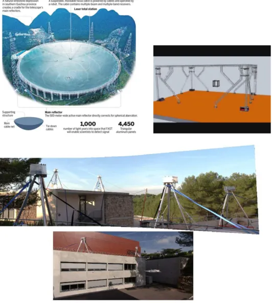
Cables are essential elements in cable-driven parallel robots (CDPR) in which grounded winches independently pay off and reel in cables wound on a drum and attached to a moving platform at the other end. Such a robot has the advantages of parallel robots (accuracy, high velocity, large payload) but also may exhibit large workspace as illustrated by the FAST telescope robot [1], the COGIRO robot of Tecnalia/LIRMM [2] and our MARIONET-CRANE prototype [3] (figure 1).
Most of the works related to CDPR assume ideal cables without elasticity and deformation due to the cable mass. With that model the distance Lr
between the attachment point B of the cable on the CDPR platform and the winch output point A is exactly the paid off cable length L0 as measured.
However the no-elasticity assumption does not hold for large CDPR with a difference between L0, Lr of several centimeters or a variation evaluated at
Figure 1: Large CDPR: the FAST telescope, the COGIRO robot and our MARIONET-CRANE prototype. The sagging effect on the later CDPR may easily be seen in the video part of the Hephaistos web site.
1% for a small CDPR [4]). As we will see the deformation of the cable due to its own mass induces also significant changes (see figure 3). Neglecting these effects will incur significant errors on the positioning of the CDPR but also on other state variables of the robot such as cable tensions or velocities. In this paper we will consider the elasto-static Irvine sagging cable model that has been proposed for elastic and deformable cable with mass [5] and that has been shown to be in very good agreement with experimental re-sults [6]. This model assumes that the cable lies in a vertical plane, the cable
plane, and is therefore a 2D model. There are also other models that take into account torsion, out-of-plane motion [7, 8], the multi-strand nature of the cable [9] or specific to synthetic rope [9, 10, 11, 12, 13] but they are mostly valid for cables with a much larger diameter than the one used for CDPR or for cables having a very specific structure. Lumped-mass model have also been proposed [14] but we will see that they are difficult to use for CDPR.
A global reference frame O, (xr, yr, zr) is defined, with z corresponding
to the upward local vertical, and a cable reference frame Ai, (x, z = zr) is
defined in this plane with its origin at Ai, one of the extremity of the cable
and x in the cable plane, being perpendicular to z = zr . The coordinates
of the other cable extremity Bi are (xb ≥ 0, zb) and we will assume that Bi
is below Ai so that zb ≤ 0 (Assumption 1). Vertical and horizontal forces
Fz, Fx > 0 are exerted by the platform on the cable at point Bi (figure 2).
x yr z= zr A Fx Fz O F B(xb, zb) zr xr u
Figure 2: Notation for a sagging cable
Note that Fz is negative if the platform is exerting a downward force at B
(the tangent of the cable at B has a negative z component), while Fz is
For a cable with length at rest L0 the coordinates of B are given by the Irvine equations [5]: xb = Fx( L0 EA0 + sinh −1(Fz Fx)− sinh −1(Fz−µgL0 Fx ) µg ) (1) zb = FzL0− µgL20/2 EA0 +pF 2 x + Fz2−pFx2+ (Fz− µgL0)2 µg (2)
where E is the Young modulus of the cable material, A0 the cable
cross-section area and µ the cable linear density. For example we may illustrate the influence of the cable deformation for a steel cable of diameter 6mm, length L0 = 50 meters with infinite E (and therefore no elasticity) and
µ = 0.346kg/m under a tension of 100 N by plotting the difference L0−Lras
a function of Fx (figure 3). As may be seen in the figure there is a significant
difference between L0 and Lr and this change will directly affect the CDPR
platform positioning.
Figure 3: Difference in meter between the cable length and the distance between the attachment points A, B as function for Fx (N) for a total tension of 100N and a cable
length at rest of 50 meters. This figure clearly shows that the sagging effect induces a large difference between the measured cable length and the distance between A, B as soon as Fx increases.
difference between the distance between A, B and the cable length. Neglect-ing these effects will introduce error in the kinematic analysis of CDPR.
Another interesting property of the Irvine equations is that when E → ∞, µ → 0, then they provide exactly the ideal cable model [15]. This point has been used in [15], [16] to propose algorithms for solving the inverse and direct kinematics of CDPR. The main idea of these algorithms is to start with the solutions of these problems for ideal cables (ie. E = ∞, µ = 0) and for each of these solutions to incrementally move E, µ toward their real values, using a guaranteed Newton scheme to find the new solution at each step. Another interest of the Irvine equations is that they provide a very compact description of the cable effect with very few physical parameters, namely E, µ. The µ parameter may easily been estimated accurately, while E is more difficult to estimate and is time-varying. However we believe that an auto-calibration of E (which is outside the scope of this paper) based on additional sensors giving information on the state of the robot (see [17] for example) is doable. On the other hand using the lumped-mass model [14] will require much more parameters (number and location of the nodes, mass and spring stiffness) that are difficult to estimate and has never been proven experimentally for CDPR. Furthermore the low number of parameters in the Irvine equations allows one to manage uncertain values with interval analysis, while increasing the number of parameters will make this task much more difficult.
Equations (1,2) have as variables xb, zb, L0, Fx, Fz. In the remaining
sec-tions of this paper we will consider that a combination of these variables have known values and we will determine closed-form solution for the re-maining variables or univariate polynomials in one of the variable for which the maximal number of roots will be established. Some works have addressed this topic especially assuming that 3 of these 5 variables have a fixed value and establishing 2 equations for the remaining variables[18] whose solution is determined numerically. Our first contribution will be to establish new relationships between the variables that have not, to the best of the author knowledge, been proposed before.
Our second contribution addresses the use of these new relationships for the solving of the inverse and direct kinematics (IK and DK) of CDPR for which the cable model will obviously play an essential role. Cable model also influences the static analysis whose purpose is to determine the tension in the cables [19].
the cable plane and the xb, zb of each cable are known) with the purpose
of determining L0. One may notice that (1,2) in their current form do not
provide a closed-form for L0. Hence solving the IK requires solving an
equa-tion system in 2n equaequa-tions (1,2) with 3n unknowns and of the mechanical equilibrium of the platform that imposes 6 additional equations. If n = 6 we end-up with a square system of equations [20],[21],[22], To solve the IK authors have used optimization or have assumed that the solution is suffi-ciently close to the rigid leg case which is therefore used as initial guess for a solving based on the Newton scheme. However these methods cannot with certainty find all the solutions (as it has already be proven that the IK may have multiple solutions).
In the DK problem the n L0 are known and the platform poses have to
be determined. The unknowns are here the 6 parameters that define the platform pose and the 2nFx, Fz while the constraints are the 2n equations
(1,2) and the 6 equations of the mechanical equilibrium, so that we have al-ways a square system that has usually multiple solutions. Note however that the DK assumes the measurement of L0 while current systems provided the
stressed length so that corrective steps should theoretically be applied. As equations(1,2) are not algebraic we cannot use methods such as elimination or Groebner basis that may provide all solutions for the DK and IK. Con-tinuation method [23] are an option but requires a starting point. A natural starting point is to consider the cables as ideal and using the solutions of the IK and DK. However singularity are crossed during the continuation and are difficult to manage [16, 24]. It was recently proposed to solve the DK by looking at the minima of the potential energy of CDPR [25] but finding numerically all these minima is tedious and uncertain.
We have addressed the IK and DK solving issues in previous publications, using as solving method an interval analysis-based approach that is guaran-teed to provide all solutions assuming that the unknowns are bounded [26, 27] and is able to manage different cable models. The next section presents the principle of solving based on interval analysis and explains how the additional relationships we will provide in this paper may speed-up the solving. Note that this paper is an extended version of the conference paper [28] with new results and examples that illustrate the use of this work for the kinematic analysis of CDPR.
2. Interval analysis
Interval analysis is based on interval evaluation of a function f in the unknowns {x1, x2, . . . xn} that are supposed to be bounded i.e. for each
xi we have xi ∈ [xi, xi] where xi, xi are respectively the lower and upper
bound for xi. Such bounds define a box in the n-dimensional space of the
unknowns. Being given such a box B the interval evaluation ˆf of f over B is an interval [f , f ] such that for any point X in B we have f ≤ f(X) ≤ f. In other words f is either equal to or a minorant of the minimum fmin of
f over B while f is equal to or a majorant of the maximum fmax of f over
B. The interval evaluation of f is relatively easy to obtain if f is expressed in terms of classical mathematical functions using the natural evaluation which basically consist in replacing the operators by interval equivalents. For example interval evaluation of the Irvine equations may be obtained by natural evaluation. A property of interval analysis is that two mathematically equivalent forms of f may have different interval evaluations. For example f1
= x2
+ 2x + 1 and f2
= (x + 1)2
are equivalent but ˆf2 will be tight with
only one occurrence of x while ˆf1 will not if x < 0. A solving algorithm
may then be designed just by discarding boxes for which we have for any equation in the set either f > 0 or f < 0 as this shows that there is no solution of this equation for the variable in the box. Otherwise the box is bisected: one variable is chosen and its range is bisected at its mid -point so that two new boxes are created differing just by this variable range. It is not needed to bisect a box until it is reduced to a point as sophisticated methods [29, 30, 31, 32] allow to determine if a single root is present in a box (provided that it is small enough) and provide a numerical method to calculate this root.
However the efficiency of interval algorithms is drastically dependent upon the tightness of the interval evaluation: the closer f , f are to fmin, fmax, the
faster will be the algorithm. An interval evaluation will be denoted tight if ˆf = [fmin, fmax]. But the natural evaluation may lead to large under or
overestimation of the minimum and maximum as soon as there are multiple occurrences of the unknowns in f (it may be proven that if there is only a single occurrence of each unknown in f , then ˆf is tight, up to round-off errors). The tightness will improve when the widths of the intervals for the unknowns decrease but an efficient way to improve the tightness of the evaluation is to consider the derivatives of f and their own interval evaluation. Let fi be the derivative of f with respect to xi and let [fi, fi] be its interval
evaluation overB. If fi > 0 or fi < 0, then f is monotonic with respect to xi.
Consequently ˆf may be obtained as [Min ˆf (Bi), Max ˆf (Bi)] where Bi are the
boxes that are derived from B with xi set to xi or xi. Note that this process
has to be applied recursively. Indeed assume that there is a j > 1 such that f is monotonic with respect to xj (implying that ˆf will be obtained using
Bj), while for i < j this was not the case. But for i < j the monoticity has
been evaluated usingB and as we are now using the tighter Bj the monoticity
test may give another result. Using this process we may tighten the interval evaluation of f up to the point where ˆf = [fmin, fmax] if f is such that all
fi, i ∈ [1, n] are positive or negative. Besides the use of derivatives another
method is usually efficient to decrease the computation time. Let us assume that an equation may be rewritten as H(xi) = G(x1, . . . xi−1, xi+1. . . xn)
where H is an invertible function of xi. Let ˆG = [G, G] be the interval
evaluation of G for a given box. The range ˆxi for the unknown xi is updated
by ˆxi ∩ H−1( ˆG) and the box is discarded if this intersection is empty. We
may also sharpen the range for xi by computing [xi, xi+ ǫ]∩ ˆG where ǫ is a
small value: if this intersection is empty then the lower bound for xi becomes
xi+ ǫ and we may repeat the process. A similar procedure may be used for
the upper bound.
One difficulty of interval analysis is determining the right combination of heuristics that leads to the best computation time being given that this heuristics may reduce the computation time of the basic interval analysis algorithm from an almost intractable value to a few seconds.
Our second contribution is to present in the next sections some interesting properties of the Irvine equations that can be used for analysis or solving purposes.
3. Properties of the Irvine equations
A preliminary property will play an important role: we have assumed that B has an altitude that is equal or lower to the one of A with the direct consequence that Fz ≤ µgL0/2 (Fz must be lower than this value as soon as
B is lower than A).
3.1. Derivatives of the Irvine equations
The sign of the derivatives of the Irvine equations may be obtained with interval evaluation but it is interesting to determine beforehand if they may be inherently monotonic.
Under assumption 1 we may establish the sign of derivatives of equations (1),(2) that will be presented without proof as they are trivial. We have
∂zb ∂L0 < 0 ∂zb ∂Fz > 0 ∂zb ∂Fx > 0 (3)
As all derivatives of zb have a constant sign, then its interval evaluation
for interval values for Fx, Fz, L0 will always be tight and can be computed
efficiently using only floating point operators. This may have an impact on the IK solving in which zb has a fixed value: If ˆzb ∩ zb =∅, then (2) has no
solution for the current Fx, Fz, L0 box. We have also:
∂xb ∂L0 > 0 ∂xb ∂Fz > 0 ∂xb ∂Fx > 0 (4)
It may also be interesting to consider the distance D = x2 b + z
2
b between A
and B. We have ∂D/∂L0 > 0 but no general monotonicity can be obtained
with respect to Fx, Fz.
Let Fx, Fz, L0 being bounded i.e. Fx ∈ [Fx, Fx], Fz ∈ [Fz, Fz], L0 ∈
[L0, L0]. Let us assume that zbis fixed and consider the equation f (L0, Fz, Fx)−
zb = 0. Using the implicit value theorem it may be shown that the solution
of this equation satisfies
∂Fx
∂L0
> 0 ∂Fx ∂Fz
< 0
so that Fx is restricted to lie in the interval [Fx′, Fx′] where Fx′ is the solution
of (2) obtained for L0 = L0, Fz = Fz and Fx′ is the solution of (2) obtained for
L0 = L0, Fz = Fz. The range for Fx may therefore be calculated as [Fx, Fx]∩
[F′
x, Fx′] and the equation has no solution if this intersection is empty. More
generally if we consider (2) when 2 of the unknowns are fixed and denotes its solution by S in the last unknown we get [L′
0, L′0] = [S(Fx, Fz), S(Fx, Fz)]
and [F′
z, Fz′] = [(S(Fx, L0), S(Fx, L0)].
3.2. New forms for the Irvine equation
We present in this section various new relationships between the quan-tities appearing in the Irvine equations. They are usually expressed in a semi-explicit form H(X) = G(Y ) where X is an element of the set{xb, zb, Fx, Fz, L0}
while Y is the complementary of X with respect to this set. The function H will be invertible and its definition may impose some constraint on G. In the numerical examples we will set E = 111
N/m2
, µ = 0.346kg/m and the cable diameter to 6 mm.
3.2.1. Using the zb equation Fx as function of zb, Fz, L0. Let a2 = F2 x + F 2 z b 2 = F2 x + (Fz− µgL0) 2 a2 − b2 = µgL0(2Fz− µgL0) < 0
then zb may be written as
zb = ( (a− b) µg )( (a + b) 2EA0 + 1) = L0(2Fz− µgL0) 2EA0 + a− b µg (5)
Let us assume now that zb, Fz, L0 are given so that (2) has only Fx as
unknown. Our objective is to get an expression of this unknown. Let us define a2 = F2 x + F 2 z b 2 = F2 x + (Fz− µgL0) 2 U = L0(Fz− µgL0/2) EA0 − z b
so that equation (2) may be written as
U + (a− b) µg = 0 (6) We have also a2 − b2 = 2FzµgL0− (µgL0) 2 = V = (a + b)(a− b) = (a + b)(−Uµg) from which we get
b =− V Uµg − a Reporting b in (6) leads to
2a =−Uµg − V
Uµg = W (7)
Note that U, V are not function of Fx so that W is expressed only as a
function of Fz, L0. As a 2 = (W/2)2 = F2 x + F 2 z we get F2 x = (W/2) 2 − F2 z (8)
where the right-hand term is a function of Fz, L0 only. This equation provides
Fx if zb, L0, Fz are fixed but also imposes a constraint on (W/2)2 − Fz2 that
Let’s assume that Fz has an interval value and consider P = Fx2 =
(W/2)2
− F2
z that is positive. The polynomial P is of degree 4 in Fz and
factors out in 4 terms that are linear in Fz. The roots of P are
s1 = µgL0 2 + µgA0Ezb 2A0E + µgL0 s2 = µgL0 2 + (zb− L0) A0E L0 and s3 = µgL0 2 + (zb+ L0) A0E L0 s4 = µgL0 2 − µgA0Ezb 2A0E− µgL0
If we assume 2A0E > µgL0 then the roots in Fz are ordered as s2, s1(<
µgL0/2), s4(> µgL0/2), s3 and P will be positive if Fz ∈ [s2, s1]. If 2A0E <
µgL0then the roots are ordered as s2, s4(< µgL0/2), s1(< µgL0/2), s3.
There-fore there are 2 possible ranges for Fz leading to a positive P : [s2, s4],
[s1, µgL0/2]. The previously determined range for Fz may be used to
up-date the range of several variables in an interval analysis based algorithm. Numerical example: Consider the case where L0 ∈ [50, 50.4], Fx ∈
[100, 130], Fz ∈ [−130, −100]. The interval estimation of zb based on
equa-tion (2) is [-54.954,-30.586]. Using equaequa-tion (8) leads to the range [0,286.34] for Fx. But if we restrict zb to the range [-54.954,-49] or [-37,-30.586] the
range for Fx as deduced from (8) does not have an intersection with the
range [100,130]. Therefore we can claim that zb is restricted to ]-49,-37]: this
interval is 7 times smaller than the one that has initially been obtained. L0 as function of zb, Fz, Fx.
We are now interested in determining L0 when Fx, Fz, zb are fixed. Let U1 =
pF2
x + Fz2, U2 = µgFz/EA0, U3 = (µg) 2
/(2EA0) and U4 = −µgzb + U1.
Equation (2) may be written as
U2L0− U3L 2
0+ U4 =pFx2+ (Fz− µgL0)2 (9)
Squaring the previous equation leads to Ps = (U2L0− U3L 2 0+ U4) 2 − (F2 x + (Fz− µgL0) 2 ) = 0 (10) As U1, U2, U3, U4 are not functions of L0 > 0 this equation is a fourth order
polynomial in L0. Using the Sturm sequences it is possible to show that Ps
has only 2 roots for L0 in the range [0,∞]. One of these root leads to
U2L0− U3L 2
that is not compatible with equation (9). Therefore solving Ps (whose roots
may be obtained in analytical form but cannot be displayed here for lack of space) leads to a single solution for L0. Note that for an interval-based
algorithm we will first compute an interval evaluation of Ps to determine
if it may have a zero and it is not necessary to use the analytical form of the roots to obtain bounds for L0 using only the interval evaluation of the
polynomial coefficients [33, 34]. As we may have a tight range for L0 (e.g. in
the DK problem) another possibility is to look at the Sturm sequences (or at the simpler Budan-Fourier sequence) of the polynomial for this range. whose elements are functions of Fx, Fz. If there is no root to the polynomial (10),
then the number of sign changes for L0 minus the number of sign changes for
L0 should be equal to 0, thereby inducing inequality constraints on Fx, Fz
that may possibly allow one to tighten the ranges for these variables.
Numerical example: we assume that L0 is measured and lie in the
range [50,50.03] meter . A sensor on the platform allows to get an estimation of zb as -42.3922 ± 0.05 meter. The force Fx is estimated to be in the range
[100,110] while Fz is in the range [-130,-110]. An analysis of the
Budan-Fourier sequence for L0 = 50 and L0 = 50.03 shows that the polynomial Ps
has a root in the L0 range only if Ps(50)× Ps(50.03) < 0. An analysis of
the derivatives of Ps with respect to Fx, Fz shows that they are positive. As
for Fx = 110, Fz = −110 we have Ps([50, 50.03]) < 0 we deduce that the
polynomial Ps has no root whatever the values of Fx, Fz in their respective
range are.
Fz as function of zb, Fx, L0.
We consider determining Fz for given L0, Fx, zb. Equation (8) is a 4th order
polynomial Q in Fz with the constraint that W > 0. Using Budan-Fourier
theorem [33] it is possible to show that Q has 0 or 2 roots in the range ]− ∞, µgL0/2] but only one these roots will lead to a positive W > 0. The
analysis of the sign of W is complex but it may be shown that if EA0 ≫ µgL0,
then Fz must belong to the range [µgL0/2+EA0zb/L0, µgL0/2−µgzb2/(2L0)].
3.2.2. Using the xb equation
Fz as function of xb, Fx, L0.
We consider the calculation of Fz being given Fx, L0, xb. We define
u = Fz Fx
v = Fz− µgL0 Fx
so that equation (1) may be written as
(xb Fx −
L0
EA0
)µg = sinh−1(u)− sinh−1(v) (11)
We define H1 = xb/Fx− L0/(EA0) and we use the identity
sinh−1(u)− sinh−1(v) = sinh−1(u√1 + v2− v√1 + u2)
Using the the hyperbolic sine of both terms of equation (11) we obtain: H(xb, L0, Fx) = sinh(H1µg) = u
√ 1 + v2
− v√1 + u2 (12)
We have already defined a2
= F2 x + F 2 z, b 2 = F2 x + (Fz − µgL0)2 so that a2 = F2 x(1 + u 2 ) and b2 = F2 x(1 + v 2
). Equation (12) may therefore be written as:
FxH(xb, L0, Fx) = ub− va (13)
Note that the left-hand term of this equation is not a function of Fz. Let us
define W = FxH(xb, L0, Fx) and u1, u2 such that 1 + u2 = u21, 1 + v 2 = u2 2 so that W = ub− va = Fzu2− u1(Fz− µgL0) (14) We have also u2 1− u 2 2 = u 2 − v2 so that u2 1− u 2 2 = (2FzµgL0− (µgL0) 2 )/F2 x (15)
Solving (14) for u2and reporting it in (15) leads to an equation in u1, Fx, Fz, L0, W
which is of second order in u1. Substituting u21 = (F 2 x + F 2 z)/F 2 x in this
equa-tion lead to a linear equaequa-tion in u1. This equation is solved in u1 and the
result is reported in u2 1 = (F 2 x + F 2 z)/F 2
x that becomes a polynomial of order
4 in Fz whose coefficients are functions of Fx, L0, xb
L0 as function of xb, Fx, Fz.
Consider equation xb − xsb where x s
b is a desired value for xb and xb is
provided by equation (1) and Fx, Fz are given. This equation may be written
as
F (L0) = u2L0− u3sinh−1(u4+ u5L0)− u1 = 0 (16)
with −u1 = xsb/Fx− sinh−1(Fz/Fx)/(µg), u2 = 1/(EA0) > 0, u3 = 1/(µg) >
a closed-form for the root in L0 of this equation, it appears that F has
interesting properties. Indeed the derivative of F with respect to L0 is strictly
positive, while F (0) = −xs
b/Fx < 0, and consequently there is a single root
in L0 for F = 0. Furthermore as the term u2L0 is positive if−u3sinh−1(u4+
u5L0) > u1, then F > 0. Further manipulation of this inequality leads to
F > 0 if L0 > |u5|sinh−1(u1/u3)/u4 = LM0 . Hence LM0 is an upper bound
for the root of F = 0. A simple dichotomy procedure allows one to obtain quickly an estimation of the root. At each step of the dichotomy we check if the Kantorovitch theorem conditions [35] hold for the current estimation of the root so that the Newton scheme will converge to the solution. Such a procedure leads to a very fast determination of the root, that may be obtained with an arbitrary accuracy. If Fx, Fz are provided as intervals, then
rewriting F as L0 = (u3sinh−1(u4+ u5L0) + u1)/u2may be useful to decrease
the range for L0.
Numerical example: we set Fx = 1, Fz = −10, xsb = 0.5. We obtain
LM
0 = 18.571. For Lm0 /2 we get F < 0 so that we set L0 = (LM0 /2 + LM0 )/2 =
13.92855. For that value the Kantorovitch conditions hold and the Newton scheme provide the solution L0 = 13.1732.
Fx as function of xb, L0, Fz.
Consider equation xb − xsb where xsb is a desired value for xb and xb is
provided by equation (1) and L0, Fz are given. It seems difficult to derive
a closed-form for the root in Fx of this equation. But we have shown in
section 3.1 that ∂xb/∂Fx is positive. As the limit of xb when Fx goes to 0 is
0 while its limits when Fx → ∞ is L0. Hence this equation has a single root
in Fx.
We note also that xb = FxL0/(EA0)+α where α is positive. Consequently
we have FxL0/(EA0) < xb or Fx < EA0xb/L0, this inequality providing an
upper bound for the root of Fx. Hence a dichotomy process, mixed with the
use of the Newton method as described in the previous section, will provide efficiently the root.
3.2.3. Using the xb and zb equations
We proceed along the same direction than the calculation of Fz described
in section 3.2.2 using the equation
FxH(xb, L0, Fx) = ub− va (17)
We have already established in section 3.2.1 the values of a, b as functions of zb, L0, Fz while u, v are functions of Fx, L0, Fz. Hence the right-hand term of
(17) is a function of zb, L0, Fx, Fz. This function is a third order polynomial
P3 in Fz. Using the Sturm sequence [33] and the constraint a > 0 it is
possible to show that P3 has a single real root in the range ]− ∞, µgL0/2].
Numerical example: we assume xb ∈ [24.65, 24.8], zb ∈ [−43.5, −43],
Fx ∈ [90, 100], Fz ∈ [−90, −85] and L0 ∈ [49, 49.02]. The number of sign
changes of the Budan-Fourier sequence for Fz =−90 and for Fz =−85 are
both one so that P3 has no root in its interval.
zb as a function of xb, Fx, Fz, L0.
Equation (2) provides a mean of calculating zb when Fx, Fz, L0 are known
but does not involve xb and we provide here another form that involves xb.
Using the notation and result of section 3.2.3 we get:
zb = L0 Fz (pF2 x + Fz2− F2 x µgL0 sinh(µg(xb Fx− L0 EA0 ))) +L0(Fx− µgL0/2) EA0 (18)
Note that we may also obtain a bound on the cable tension pF2 x + F 2 z at B as pF2 x + Fz2 = F2 x µgL0 sinh(µg(xb Fx − L0 EA0 )) + Fz( zb L0 + µgL0 2EA0 − Fz EA0 ) (19)
3.3. Using the cable tangents
Sensors may provide a relatively accurate measurement of the cable tan-gents v = (Fz − µgL0)/Fx at A and u = Fz/Fx at B [17]. Under the
assumption that u, v are known we get
Fx = µgL0 (u− v) Fz = uFx F 2 x + F 2 z = ( µgL0 (u− v)) 2 (1 + u2 ) (20)
A trivial transformation of (2) leads to:
µ gL0 2 (u + v) + 2 A0EL0( √ u2+ 1 −√v2+ 1) + 2 z bEA0(v− u) = 0 (21)
which is a quadratic polynomial in L0 whose coefficients are functions of
u, v, zb. It is easy to show that this polynomial has a single positive root.
Now equation (1) may be written as
Fx( L0 EA0 +(sinh −1(u)− sinh−1(v)) µg )− xb = 0 (22) As we have Fx = µgL0/(u− v) this equation may be transformed in a second
order polynomial in L0 whose coefficients are functions of u, v, xb. Here again
it is easy to show that this polynomial has at most one positive root.
As Fz = uFx and L0 = (Fx(u− v))/(µg) equations (11), (22) are
polyno-mials in Fx with coefficients that are functions of u, v. The resultant of these
equations in Fx establishes a polynomial relationship between xb, zb which is
a quadric, more precisely a parabola which is written as (Axb+ Czb)
2
+ Dxb+ F zb = 0 (23)
with
A = √µg(u− v)(u + v) C =−2√µg(u− v) D = 2EA0(u− v)(R1µg(u + v)− 2R2)R2
F = −2µgEA0(u− v)(R1µg(u + v)− 2R2)R1
R1 = (sinh−1(u)− sinh−1(v))/(µg) R2 =
√
1 + u2−√1 + v2
Note that if EA0 ≫ µgL0, then A, C are small and D, F very large so that
the parabola is very close to a line.
The measurements of u, v.L0provide a direct estimation of Fx = µgL0/(u−
v) and consequently of Fz = uFxand therefore of the cable tension at B
with-out any force sensor. As these measurements are uncertain (however with a bounded uncertainty) we will get a range for xb, zb using equations (1,2)
that may possibly be sharpened using the parabola equation (23). These sharpened evaluations may possibly be used to sharpen either L0, u, v and/or
Fx, Fz.
3.4. Summary
Each of the two Irvine equations involves 4 variables: xb (or zb), Fx, Fz, L0.
Consequently each equation may be used to determine one of the variables if the other 3 variables are known. If both equations are used we have 5 variables. If 3 of them are known the Irvine equations become a system of 2
equations in 2 unknowns and we may, theoretically, obtain these 2 unknowns as functions of the known variables. We have not been able to reach this goal (except for the trivial case where xb, zb are the unknowns). However if
we assume that 4 variables are known, then the Irvine equations are over-constrained and may be used to calculate the remaining unknown. Table 1 summarizes the obtained result. In this table the unknown are presented as Fx, Fz, L0, xb, zb. For one unknown there are several columns. Each of this
column is either empty or has a • or a ÷ symbol. A column with only • indicates that the unknown can be calculated in closed-form if the indicated variables are set. A column with only ÷ indicates that the unknown has not been obtained in closed-form but that an efficient numerical scheme can be designed to calculate the unknown. For example the first column for the unknown Fx shows that Fx can be calculated in closed-form if Fz, L0, zb are
known, while the second column shows that Fx can be calculated numerically
if Fz, L0, xb are known. Fx Fz L0 xb zb Fx - • • • • ÷ • • • Fz • ÷ - • ÷ • • • L0 • ÷ • • • - • • • xb ÷ • • ÷ - • zb • • • •
-Table 1: Summary of the result showing how the unknown indicated in the first row can be be obtained as function of the variables indicated in the first vertical column.
4. Conclusion
We have presented in this paper various results regarding the Irvine equa-tions that may be useful both for analysis and solving of kinematic equaequa-tions that rely on this cable model as they establish a more general view of the underlying structure of this model. We have shown that the proposed new forms of the Irvine equations may be useful to speed up the solving of the IK and DK of CDPR based on interval analysis (part of them have been implemented our CDPR IK and DK solver with a strong influence on the solving time for finding all solutions). But they may possibly also be used for alternate solving methods such as continuation. It must be reminded that
all these solving methods are not intended to be used for real-time computa-tion (i.e. within the sampling time of the CDPR controller) as generic and guaranteed Newton scheme exists for that purpose. Still open issues on the CDPR with sagging cables such as workspace and singularity analysis may benefit from this new approach to the Irvine equations.
Acknowledgement:
This paper has been partly supported by Agence Nationale de la Recherche (ANR), under grant ANR-18-CE10-0004-03 (CRAFT project)
References
[1] X. Tang, R. Yao, Dimensional design of the six-cable driven parallel ma-nipulator of FAST, ASME J. of Mechanical Design 133 (11) ( November 2011) 111012–1/11.
[2] M. Gouttefarde, D. Nguyen, C. Baradat, Kinetostatics analysis of cable-driven parallel robots with consideration of sagging and pulleys, in: ARK, Ljulbjana, June 29- July 3, 2014, pp. 213–221.
[3] J.-P. Merlet, D. Daney, A portable, modular parallel wire crane for rescue operations, in: IEEE Int. Conf. on Robotics and Automation, Anchorage, May, 3-8, 2010, pp. 2834–2839.
[4] V. Schmidt, A. Pott, Investigating the effect of cable force on winch winding accuracy for cable-driven parallel robots, Proceedings of the Institution of Mechanical Engineers, Part K: Journal of Multi-body Dy-namics 230 (3) (2016) 237–241.
[5] H. M. Irvine, Cable Structures, MIT Press, 1981.
[6] N. Riehl, et al., On the determination of cable characteristics for large dimension cable-driven parallel mechanisms, in: IEEE Int. Conf. on Robotics and Automation, Anchorage, May, 3-8, 2010, pp. 4709–4714. [7] M. Ahmadi-Kashani, A. Bell, The analysis of cables subject to uniformly
distributed loads, Eng. Struct. 10 (1988) 174–182.
[8] H. Hussein, M. Gouttefarde, F. Pierrot, Static modeling of sagging ca-bles with flexural rigidity and shear forces, in: ARK, Bologna, July, 1-5, 2018.
[9] S. Ghoreishi, et al., Analytical modeling of synthetic fiber rope. part II: a linear elastic model for 1+6 fibrous structure, Int. J. of Solids and Structures (2007) 2943–2966.
[10] J. Piao, et al., Open-loop position control of a polymer cabledriven parallel robot via a viscoelastic cable model for high payload workspaces, Advances in Mechanical Engineering 9 (12).
[11] W. Samuel, et al., Synthetic mooring rope for marine renewable energy applications, Renewable energy 83 ( November 2015) 1268–1278. [12] V. Schmidt, Modeling techniques and reliable real-time implementation
of kinematics for cable-driven parallel robots using polymer fiber cables, Ph.D. thesis, Universit´e Stuttgart ( June, 20, 2016).
[13] P. Tempel, F. Trautweing, A. Pott, Experimental identification of stress-strain material models of UHMWPE fiber cables for improving cable tension control strategies, in: ARK, Bologna, July, 1-5, 2018.
[14] J. Kamman, R. Huston, Multibody dynamics modeling of variable length cable systems, Multibody System Dynamics 5 (3) (2001) 211– 221.
[15] J.-P. Merlet, A new generic approach for the inverse kinematics of cable-driven parallel robot with 6 deformable cables, in: ARK, Grasse, June, 27-30, 2016.
[16] J.-P. Merlet, Preliminaries of a new approach for the direct kinemat-ics of suspended cable-driven parallel robot with deformable cables, in: Eucomes, Nantes, September, 20-23, 2016.
[17] J.-P. Merlet, An experimental investigation of extra measurements for solving the direct kinematics of cable-driven parallel robots, in: IEEE Int. Conf. on Robotics and Automation, Brisbane, 2018.
[18] D. Papini, On shape control of cables under vertical static loads, Mas-ter’s thesis, Lund University, Lund (2010).
[19] L. Hui, A giant sagging-cable-driven parallel robot of FAST telescope: its tension-feasible workspace of orientation and orientation planning, in: 14th IFToMM World Congress on the Theory of Machines and Mecha-nisms, Taipei, October, 27-30, 2015.
[20] K. Kozak, et al., Static analysis of cable-driven manipulators with non-negligible cable mass, IEEE Trans. on Robotics 22 (3) ( June 2006) 425–433.
[21] N. Riehl, et al., Effects of non-negligible cable mass on the static be-havior of large workspace cable-driven parallel mechanisms, in: IEEE Int. Conf. on Robotics and Automation, Kobe, May, 14-16, 2009, pp. 2193–2198.
[22] D. Sridhar, R. Williams II, Kinematics and statics including cable sag for large cable suspended robots, Global Journal of Researches in Engi-neering: H Robotics & Nano-Tec 17 (1).
[23] E. Allgower, Numerical continuation methods, Springer-Verlag, 1990. [24] J.-P. Merlet, A generic numerical continuation scheme for solving the
direct kinematics of cable-driven parallel robot with deformable cables, in: IEEE Int. Conf. on Intelligent Robots and Systems (IROS), Daejeon, October, 9-14, 2016.
[25] A. Pott, P. Tempel, A unified approach to forward kinematics for cable-driven parallel robots based on energy, in: ARK, Bologna, July, 1-5, 2018.
[26] J.-P. Merlet, The kinematics of cable-driven parallel robots with sag-ging cables: preliminary results, in: IEEE Int. Conf. on Robotics and Automation, Seattle, May, 26-30, 2015, pp. 1593–1598.
[27] J.-P. Merlet, On the inverse kinematics of cable-driven parallel robots with up to 6 sagging cables, in: IEEE Int. Conf. on Intelligent Robots and Systems (IROS), Hamburg, Germany, September 28- October 2, 2015, pp. 4536–4361.
[28] J.-P. Merlet, Some properties of the Irvine cable model and their use for the kinematic analysis of cable-driven parallel robots, in: EUCOMES, Aachen, September, 4-6, 2018.
[29] E. Hansen, Global optimization using interval analysis, Marcel Dekker, 2004.
[30] L. Jaulin, M. Kieffer, O. Didrit, E. Walter, Applied Interval Analysis, Springer-Verlag, 2001.
[31] J.-P. Merlet, ALIAS: an interval analysis based library for solving and analyzing system of equations, in: SEA, Toulouse, June, 14-16, 2000. [32] A. Neumaier, Interval methods for systems of equations, Cambridge
University Press, 1990.
[33] P. Ciarlet, J.-L. Lions, Handbook of numerical analysis, 7 : solution of equations in Rn (part 3), North-Holland, 2000.
[34] J.-P. Merlet, Determination of the minimal and maximal real roots of parametric polynomials using interval analysis, in: 1st Int. Workshop on Global Constrained Optimization and Constraint Satisfaction (Co-cos’02), Valbonne, October, 2-4, 2002, published in LNCS Volume 2861 / 2003,pp. 71-86.
[35] R. Tapia, The Kantorovitch theorem for Newton’s method, American Mathematic Monthly 78 (1.ea) (1971) 389–392.