Decision making under epistemic uncertainty : an application to seismic design

Decision Making under Epistemic Uncertainty:

An Application to Seismic Design

by

Anna Agarwal

Bachelor of Technology in Civil Engineering (2005) Indian Institute of Technology-Delhi, India

Submitted to the Department of Civil and Environmental Engineering in partial fulfillment of the requirements for the degree of Master of Science in Civil and Environmental Engineering

at the

MASSACHUSETTS INSTITUTE OF TECHNOLOGY February 2008

© 2008 Massachusetts Institute of Technology. All rights reserved.

Author:...

Certified by:.. .

. . .. . . . . . . .. . . . . ... ... .. ... . .

Department of Civil and Environmental Engineering December 17, 2007

.. .v- ,-, _{D ...e}

Daniele Veneziano Professor of Civil and Environmental Engineering Thesis Supervisor

Accepted by:.

K~f.,

.. . . .... . . . .. .. . . ... . Daniele Veneziano Chairman, Departmental Committee for Graduate Students

ARCHIES

MASSACHUSE1180"W.

OF TEOHNOLOGY

APR 1 5 2008

Decision Making under Epistemic Uncertainty:

An Application to Seismic Design

by

Anna Agarwal

Submitted to the Department of Civil and Environmental Engineering on December 17, 2007, in partial fulfillment of the requirements for the degree of

Master of Science in Civil and Environmental Engineering

Abstract

The problem of accounting for epistemic uncertainty in risk management decisions is conceptually straightforward, but is riddled with practical difficulties. Simple approximations are often used whereby future variations in epistemic uncertainty are ignored or worst-case scenarios are postulated. These strategies tend to produce sub-optimal decisions. We develop a framework based on Bayesian decision theory that accounts for the random temporal evolution of the epistemic uncertainty and minimum safety standards, and illustrate the effects of these factors for the case of optimal seismic design of buildings. Results show that when temporal fluctuations in the epistemic uncertainty and regulatory safety constraints are included, the optimal level of seismic protection exceeds the normative level at the time of construction. We do a sensitivity analysis concerning the repair and retrofit strategies that control the repair actions following earthquake damages and the amount of structural upgrading in the case of non-compliance with the safety standards. We see, that just like the optimal initial design system, upgrades should also be made conservatively to provide a margin of safety against future adverse changes in the epistemic uncertainty and regulations. The optimal degree of conservatism depends in a complex way on the cost of providing additional seismic protection, increase in earnings from additional seismic protection, costs of repairs and upgrading, seismicity of the region and the volatility of both the estimated hazard (due to changes in epistemic uncertainty) and the regulatory environment. The effect of all these influencing factors is studied through an extreme sensitivity analysis. We argue that the optimal Bayesian decisions do not depend on the aleatory or epistemic nature of the uncertainties, but only on the total (epistemic plus aleatory) uncertainty and how that total uncertainty varies randomly during the lifetime of the project.

Thesis Supervisor: Daniele Veneziano

Acknowledgements

First and foremost, I would like to express my sincere gratitude to my advisor, Prof. Daniele Veneziano, for giving me an opportunity to work with him. His guidance and constant encouragement was very important for completion of this work. He has always encouraged me to think beyond the immediate focus of research to be able to appreciate a holistic view of the problem situation. It has been professionally enriching to learn from his vast pool of knowledge. It has truly been a privilege to work under his able guidance.

I wish to thank Erdem Karaca for helping me with an important part of this thesis. He was always there with his help and advice whenever needed inspite of his several pressing commitments. I enjoyed and benefited from the

discussions with him throughout the course of this work.

I am indeed very grateful to the East Japan Railway Company for financially supporting this study. A special thanks to Makoto Shimamura, Yayoi Misu Uchiyama and Keiichi Yamamura for the useful discussions.

I would like to thank Kris, Jeanette, Patty and Sheila for helping me with the administrative matters. I thank my office-mates for their very enjoyable and intellectual company which went beyond the Institute corridors. Very special and heartfelt thanks to all my wonderful friends for making my stay at MIT a truly cherished one.

Last but not the least, I am grateful to the most important people in my life. From the bottom of my heart I thank my parents and my little sister for their unconditional love and support that is my driving force.

Contents

2. Optimal Bayesian Decision under Epistemic Uncertainty ... 15

3. Model for the Optimization of Seismic Design ... 19

3.1. The State V ector ... ... ... 21

3.2. Structural and Nonstructural Damages... 22

3.3. State Transitions, Losses and Rewards... ... 23

4. A pplication E xam ples ... ... 27

4.1. Building Characteristics... ... ... 27

4.2. Repair/ Retrofitting Strategies and Frequency Ratios... 52

4.3. Transition Rates and Transition Probabilities... ... 54

4.4. C osts and Earnings... ... 58

5. Num erical Results ... ... 62

5.1. Base-Case ... ... ... 62

R egulatory L im its... ... 63

5.3. Sensitivity to Cost and Loss Parameters... ... 74

5.4. Changing the Retrofitting Strategy... ... 77

5.5. Changing the Repair Strategy... 79

5.6. Sensitivity to the Fixed Cost of Structural Upgrading and the Earning Rate... 80

5.7. Comments on Sensitivity Analysis... ... 84

6. C onclusions ... ... 86

List of Figures

Figure 4.1 Spectral acceleration hazard for 8 high-rise and 9 low-rise designs in

Los Angeles, California... 31

Figure 4.2a. Inelastic spectral displacements from time-history analysis and fitted conditional lognormal parameters (log mean and log mean + one log standard deviation) for high-rise designs... ... 36

Figure 4.2b. Inelastic spectral displacements from time-history analysis and fitted conditional lognormal parameters (log mean and log mean ± one log standard deviation) for low-rise designs... ... 41

Figure 4.3a. Fragility curves for different damage states for high-rise designs... 46

Figure 4.3b. Fragility curves for different damage states for low-rise designs ... 50

Figure 5.1 Return per dollar invested (RPDI) for different initial designs: base case... 64

Figure 5.2 Sensitivity to the future volatility of the epistemic uncertainty and the regulatory limit on risk... ... ... 65

Figure 5.3 Comparison of the relative economic value of different designs using the present model with no change in E and R and the model of W en and K ang [20]... 68

Figure 5.4 Sensitivity to the future rates of changes in the epistemic uncertainty and the regulatory limit on risk... .... ... 73

Figure 5.6 Sensitivity of RPDI to the rate of damaging earthquakes for

high-rise designs...76

Figure 5.7 Dependence of RPDI on the retrofitting strategy... 78

Figure 5.8 Dependence of RPDI on the repair strategy... 80

Figure 5.9 Sensitivity of RPDI to the fixed cost of retrofitting... 81

List of Tables

Table 4.1 Characteristics of high-rise and low-rise designs... 28

Table 4.2 Drift ratio and central damage factor (CDF) for different damage levels... 29

Table 4.3 Damage rates for high-rise designs in Los Angeles, California... 51

Table 4.4 Damage rates for low-rise designs in Los Angeles, California... 51

Table 4.5 Transition probabilities Pe ... 55

Table 4.6 Transition probabilities r... 56

Table 4.7 Transition probabilities Pee ... 57

3 Table 4.8 Transition probabilities Pr r"... 58

Table 4.9 Damage cost Cas ($1000) for different designs and different damage lev els... 60

Table 5.1 Expected actualized costs of high-rise and low-rise designs by the approach of W en and Kang [20]... 67

Table 5.2 Transition probabilities Pee, _{, for changes in E to occur once} every 40 years ... ... ... 70

Table 5.3 Transition probabilities Pe, ,, for changes in E to occur once every 60 years... ... 71

Table 5.4 Transition probabilities Prr,, for changes in R to occur once every 20 years... ... 71

Table 5.5 Transition probabilities Pr r", for changes in R to occur once

every 60 years... _{... 72}

Chapter 1

Introduction

Many technological and natural systems on which we depend are complex and poorly

understood. In some cases what is uncertain is the functioning of the system, while in

others it is the environment in which the system operates. In either case, the risks posed

by or to these systems are uncertain, making decisions difficult and controversial. For example, underwater ecosystems are not well studied, making it challenging to establish restoration strategies; the degree of future climate change due to human activities is

uncertain, clouding the debate on the need to control greenhouse gas emissions; and

forecasting the long-term hydrogeologic conditions at Yucca Mountain, Nevada, is

controversial, making it difficult to establish the suitability of that site as a nuclear waste

repository. Similar uncertainty clouds decisions regarding the use of new technology as

we have very little or no prior experience with its use; for example predicting the

likelihood of malfunctions in a manned expedition to Mars is not easy, raising doubts on

whether the endeavor is too risky. All these are examples of what is commonly known as

epistemic uncertainty or uncertainty due to ignorance, as opposed to aleatory uncertainty, which reflects the variability in the outcome of a repeatable experiment [1-3].

When action cannot be delayed until all epistemic uncertainties are resolved and risks

become known, one must employ decision-making strategies that account for both

aleatory and epistemic uncertainty. The strategy preferred by most risk analysts rests on Bayesian decision theory [4, 5] and takes expectation of relative frequencies and utilities over the epistemic uncertainties EP. For example, the probability of an event A is found as P[A] = E {P[A I EP]}, where P[A I EP] is the conditional relative frequency of A

EP

given the epistemic variables EP. We call this the Bayesian strategy and refer to P[A] obtained through this expectation operation as the "total probability of A", since the relation follows from the Total Probability Theorem [6, 7].

In matters of public safety, administrators often use a different strategy, based on the so-called precautionary principle [8, 9]. According to this principle, when stakes are high all epistemic variables should be set to worst-case values EPworst and decisions ranked using the conditional utility (U I EPworst).

The distinction between epistemic and aleatory uncertainty depends to some extent on the representation one makes of the events of interest, collectively referred to here as the WORLD [2]. If some of the uncertainty is represented through a stochastic model, then one views that uncertainty as aleatory and uncertainty on the form and parameters of the model as epistemic. In the limit, if the WORLD is viewed as the deterministic outcome of laws and states of nature, then all uncertainties reflect ignorance and are considered epistemic. Due to this non-unique classification of uncertainties, a desirable property of a decision strategy is that it depends on the total (epistemic plus aleatory) uncertainty and is invariant or at least insensitive to the epistemic/aleatory split.

Bayesian decisions are invariant in this respect (see Chapter 2), whereas precautionary decisions depend on the epistemic/aleatory classification because they set to worst values only the epistemic variables. An invariant version of the precautionary principle would set all epistemic and aleatory variables to worst values, thus producing even more risk-averse decisions. Another problem with the precautionary strategy is that worst-case scenarios are difficult to specify (there is always something worse one can think of). For additional arguments against the precautionary principle, see [9-11].

While theoretically well founded, the Bayesian strategy is sometimes inappropriately used. This generally happens when the utility is a nonlinear function of the level of risk and one replaces the expected utility with the utility evaluated at the expected risk [7, 12]. A frequent source of this nonlinearity is the limit imposed by society on the acceptable risk [13]. The next chapter explains in detail this concept and the effect of this non-linearity.

A rarely recognized but fundamental aspect of epistemic uncertainty in decision making is that it evolves over time. With changes in epistemic uncertainty, the estimated risk would change too and might exceed the maximum acceptable risk. To bring the system back into compliance, costly retrofit actions would then be needed. The main objective of this thesis is to develop decision strategies in the presence of such risk limits. In this thesis, the proposed model realistically allows the epistemic uncertainty and the societal limit on the acceptable risk to vary randomly with time. It is shown that due to the non zero probability of future violations of the acceptable risk limits and of incurring costly retrofits, the optimal designs tend to be more conservative than those based on the assumption that uncertainties remain the same during the lifetime of the

project. These concepts are illustrated by considering the optimal design of high-rise and

low-rise buildings against earthquake loads.

The thesis is organized as follows. Chapter 2 discusses the general principles of

optimal bayesian decision under epistemic uncertainty. These principles are exemplified

in Chapter 3 for the optimum design of buildings against earthquake loads using the

theory of Markov models with reward. High-rise and low-rise buildings in Los Angeles, California, are selected to illustrate the proposed model. The characteristics of the

building designs and the chosen model parameters are described in Chapter 4. Numerical

results are presented in Chapter 5, including an extensive sensitivity analysis with respect to the model parameters. Chapter 6 draws conclusions and suggests future research

Chapter 2

Optimal Bayesian Decision under Epistemic

Uncertainty

Suppose that a decision D is to be made to maximize some utility U(D, WORLD), where

WORLD includes all events besides D that affect U. If U depends on the future state of

uncertainty, then all the events that will determine that future state should be included in

WORLD. At any given time, WORLD is uncertain due to both epistemic (EP) and

aleatory (AL) uncertainties. In Bayesian theory, a decision is optimal if it maximizes the expectation of U(D, WORLD) with respect to all (EP + AL) uncertainties at the time to of

the decision, i.e. if it maximizes

U(D) = E [U(D, WORLD)] (2.1)

(EP+ALID,t_o)

Conditioning the epistemic and aleatory variables on D indicates that uncertainty on the future depends on what decision is made at time to. For example, using a safer design reduces the probability of future system failures. Since expectation in Eq. 2.1 is over all uncertainties, Bayesian decisions do not depend on the epistemic/aleatory classification.

Over time, with advances in knowledge, availability of more information and more sophisticated modeling tools, the epistemic uncertainty evolves and is generally reduced. The future changes in the uncertainty are difficult to predict at the time of decision.

If the consequence of the decision were to last for a short time such that no new information could become available and the state of uncertainty would remain unchanged until the rewards are collected, then what would matter for making decisions is the expected value of the risk. But a frequent aspect of design decisions involving critical systems is that decisions have long lasting consequences, as opposed to immediate rewards. For example, a nuclear waste repository must be safe for tens of thousands of years and the policies we adopt on green house gas emissions have long-term climatic impacts. In these contexts, decision makers must consider the epistemic uncertainty and its possible future evolution.

Another important aspect we need to consider while making design decisions are the constraints that might be imposed on the maximum acceptable risk of the system. Introduction of these limits causes the utility to become nonlinear function of the level of risk. To appreciate the effect of nonlinearity between utility and risk, consider a system that may operate at any future time t only if the failure rate Af(t) evaluated using total uncertainty at time t _{is below some threshold fmax (t). The assessed risk/failure rate ,f}

might change during the lifetime of the system due to changes in epistemic uncertainty. In the face of changing technology and the public attitude towards risk, the regulatory threshold on risk Af,max is subject to change as well. Whenever Af (t) > Af,max(t), one must retrofit the system to bring it back into compliance. These possible future safety violations should be included among the events in WORLD and accounted for in the

utility function U(D, WORLD), which then becomes nonlinear in 2_{f(t)[13]. Bayesian}

decision strategy is sometimes inappropriately used and the expected utility is replaced

by the utility evaluated at the expected risk. Notice that Eq. 2.1 accounts for

nonlinearities as U(D) in that equation is the expected utility and not the utility when risks are fixed to their expected values. The frequent practice of ignoring safety violations

and evaluating U(D) under the condition that Af remains constant at present values

produces unconservative decisions.

Another way to evaluate U(D) in Eq. 2.1 is to first take expectation of

U(D, WORLD) with respect to the aleatory variables AL under fixed epistemic variables EP and then take expectation with respect to EP. This gives

U(D) = E E [U(D, WORLD)] (2.2)

(EPID,to) (ALID,to,EP)

The advantage of Eq. 2.2 over Eq. 2.1 is that the conditional aleatory model of

(WORLDID, EP) that is needed to evaluate the inner expectation in Eq. 2.2 is far simpler

than the total-uncertainty model of (WORLDID) needed for Eq. 2.1. For example, if earthquake occurrences are Poisson and there is epistemic uncertainty on the earthquake rate 2, taking expectation with respect to A produces a complicated mixture of Poisson processes with non-Poisson counts and dependent non-exponential interarrival times.

Although Eq. 2.2 is operationally simpler than Eq. 2.1, when there are many epistemic variables also this way to obtain U(D) is computationally non-viable. An alternative approach is to approximate the total uncertainty model of (WORLD|D) needed

for Eq. 2.1. For example, one might replace the Poisson mixture process of earthquake

arrivals with a Poisson process having the same mean rate mi.

Simplifications of this type will be used in the calculation of U(D) for alternative

seismic designs. The next chapter illustrates the effect of non-linearity in the utility-risk

relation when risk limits are imposed by considering the problem of optimal seismic

Chapter 3

Model for the Optimization of Seismic

Design

In this chapter, we focus on the optimum seismic design of buildings. The seismic safety of a design S relative to some failure event (taken here to be partial or total collapse) is usually assessed by combining hazard and fragility information. The hazard function H(y) gives the rate at which some ground motion intensity at the site of the building exceeds various levels y and the fragility function F(y) gives the probability of building failure for different y. Given H and F, the failure rate Af(F,H) is obtained as

2f (F,H) = - F(y)dH(y) (3.1)

0

When F and H are uncertain, the total failure rate Af is the expected value of Af(F,H) with respect to the epistemic uncertainties on F and H [14, 15]. If F and H are independent, this gives

2_f

_{= - E[F(y)]E[dH(y)]}

_(3.2)

The total failure rate Af varies randomly in time due to random variations in the epistemic uncertainty (new models and theories, newly collected data, etc.) and in the system properties (for example, due to earthquake-induced damages and retrofit actions). Also the regulatory limit Af,max varies randomly in time due to changes in social standards and the heightened awareness of seismic hazards following damaging earthquakes. In order for the system to operate at any time t, the safety factor

SF(t) = f,max (t)/iAf(t) must exceed 1.

At the time of construction to, the future rates Af(t) and Af,max(t) and the future safety factor SF(t) are uncertain and are treated as random processes Af(t I to),

2_{f,max (tI to), and SF(t I to) where conditionality on to indicates that uncertainties are}

assessed at time to. These processes are complicated to analyze. Therefore, when

calculating expected utilities, we make simplifying approximations as mentioned at the end of Chapter 2.

Specifically, we approximate the total process of future earthquake events as Poisson with rate equal to the total rate calculated at time to. Similar simplifying

approximations are made for the process of failure events and the evolution of the state of the system. The true hazard function is taken to be E[H(y)] at the time of design. At later times, E[H(y)] may vary due to changes in epistemic uncertainty, but the true hazard is assumed to remain constant. We also do not dwell with the specific sources of uncertainty in H(y) (e.g. alternative seismogenic features, attenuation laws and site amplification models) and F(y) (uncertainty in the performance of structural and non-structural elements, effectiveness of connections, limiting ductility, etc.) and simply

assume a certain rate at which the assessed total failure rate Af will experience changes

in the future due to variations in any of these elements.

These simplifications should not be critical for our objective, which is to illustrate how in the presence of regulatory limits on the risk, future variations in total uncertainty affect optimal decisions. These simplifications allow one to evaluate the utility U(D) using the powerful theory of Markov processes with reward [16-18], as described next.

3.1 The State Vector

The safety factor SF(t) is a fundamental quantity in our model and must exceed 1 at all

times. Its random variation in time is due to weakening/strengthening of the system as a

result of earthquake induced damages or repair and retrofitting actions, changes in

epistemic uncertainty, and changes in the regulatory limit 'f,max. To separate these

causes of variation, we express SF(t) as the combination of three frequency ratios:

SF(t) = Fs(t) FR (t) Rf,max(t) (3.3)

A,(t) FE (t)

where

Fs(t) = Af,max (to)/ f (t I to) FE(t) = Af(t)/ 2_{f(t I to)} FR(t)= Af,max (t)/f,max (to)

The ratio F$(t) measures the safety of the system at time t using the state of uncertainty

construction. This measures the initial seismic protection level of the system and is taken as a basic variable to be optimized in design. Optimization of the repair and retrofit strategies is another objective of this thesis. For t > t_o, Fs(t) tracks the changes in

system strength due to damages, repairs, and retrofitting interventions.

The factor FE(t) is the ratio of the failure rates of the system at time t based on information at times t and t_o. Changes in this factor are caused mainly by variations in epistemic uncertainty. Finally, FR(t) tracks changes in the regulatory constraint on risk.

We view Fs, FE and FR as components of a state vector that evolves randomly in time. To facilitate calculations, we replace these continuous state variables with discrete variables S (indexing structural strength, with values 1,...,ns), E (indexing epistemic uncertainty, with values 1_{,...,nE) and R (indexing the regulatory limit on risk, with values} 1,...,nR) and denote by X = [S,E,R] the resulting state vector. Each discrete value of X is

associated with a specific value of the frequency ratios Fs,FE andFR in Eq. 3.3; see Chapter 4 for details. Low-case letters x = [s,e,r] indicate specific integer values of X and

its components. In dealing with state transitions, we generally use primed symbols (e.g.

x') for initial values and double-primed symbols (e.g. x") for terminal values.

3.2 Structural and Nonstructural Damages

As a result of earthquakes, the system may sustain structural damages. Depending on the repair strategy, the system is returned to pre-earthquake conditions or strengthened to a higher level [18, 19]. If one tracked structural damage through an additional state variable, the resulting state vector would be excessively large. To save on storage and

computation, we condense out the structural damage levels depending on what repair is made. This is done by creating a duplicate state variable S* of S and considering S = s' to

transition to S* = s" whenever, as a result of structural damages and repairs, the system is brought from state s' to state s". In this way no approximation is made and the number of possible state values is only doubled. Once in S* = s", the system has the same properties as if it were in S = s" and the roles of S and S* reverse. This is the familiar technique to

account for repairs in Markov models with reward [16, 17], which we extend here to include multiple possible damage levels. In what follows, the S* states are included in the

S state variable, which thus has 2n_s possible values. The system has a total of

n = 2nsnEn_R - nina possible states, where nina is the number of states that are

inadmissible because they violate the constraint SF > 1.

In addition to structural weakening and strengthening, one must consider non-structural losses (including damage to non-non-structural building components, economic losses from downtime, social losses from injuries and fatalities etc.). One could use additional state variables to track such nonstructural damage conditions, but if damages are instantly repaired and losses are instantly incurred one can account for these damages and losses without further augmentation of the state vector X; see below.

3.3 State Transitions, Losses and Rewards

Changes in X originate from events of three types: (1) large earthquakes in the region, which may induce damages and subsequent repairs and may additionally trigger new studies of regional seismicity and tightening of the safety regulations, (2) studies of

regional seismicity conducted independently of earthquake occurrences in the region, which lead to changes in the epistemic uncertainty, and (3) public safety reviews made

independently of the above events, which may lead to changes in the acceptable risk level. Events of Type 1 can possibly modify all three state variables, whereas events of Type 2 and 3 affect directly only E and R, respectively (but if changes in E and R are such that the regulatory constraints are violated, then also S changes due to retrofitting).

To simplify the analysis, we assume that events of different types occur according to independent Poisson processes and that the state transitions caused by different events are independent. Then the state vector X evolves in time according to a Markov process, discrete in state and continuous in time. For each event type i (i = 1, 2, 3) one must specify the rate 2A and the transition probabilities Px, x, = Pr[x'-= x" levent of Type i].

How these rates and transition probabilities are assigned will be explained in Chapter 4 in the context of a specific application example.

Markov processes with reward allow one to further account for the benefits and costs accrued during the lifetime of the system. Such earnings and losses are discounted at a specified rate y, meaning that 1 dollar earned at a future time t is worth e-r(t-t_o)

dollars at time to.

While operating in state x, the system earns at a rate ex (dollars/year). Whenever

an event of Type 1 (an earthquake) occurs and causes a transition from state x' to state

x", a lump-sum cost Cxx ., expressed as negative earned dollars, is incurred. This lump-sum cost includes non-structural repairs as well structural repairs and improvements that are called for by the chosen repair and retrofit strategies. If the transition x'> x" can occur under different (damage, repair) scenarios, the total transition probability Px x,. is

the sum of the probabilities of all such scenarios and Cx x, is the expected cost over the

same scenarios.

Similarly, when events of Type 2 or 3 occur, a state transition may result due to changes in the calculated risk or in the regulatory limit on risk. If the changes violate the condition SF(t)2 1, the structure must be strengthened according to a specified retrofit policy, at lump-sum costs C2',x and C3, , (the dollar amounts differ from Clx,, because

events of Types 2 and 3 cause no physical damage).

What matters in the calculation of the present worth of the system is the expected earning rate e_x when the system is in state x, which is found from the rate ex and the lump-sum negative earnings CiX ,, as

3

ex = x +Li 'x"ix Cx'x, (3.4)

i=1 x"

The theory of Markov processes with reward [16, 17] says that

Qx(t),

following set of linear differential equations

dQx(t)

dt +(y)( + A)Qx(t)= ex + i Q. "x,(t) (3.5) i=1 x"

where y is the discount rate and A = Al + 2 + 3 is the total rate of events that can possibly induce state changes. The initial conditions at the time of construction t_o are

Qx (to) = for all x.

As t -> 00o, the expected actualized rewards Qx(t) approach asymptotic values

Qx,

3

(y+ )Qx =ex e + + A i ,PQI x, (3.6)

i=1 x"

Since the anticipated lifetime of a building is generally long relative to the reciprocal of the discount rate 1/y, one may use these asymptotic actualized rewards, incremented by

the (negative) cost of construction, to rank alternative designs and repair/retrofit strategies.

To exemplify the proposed methodology we consider two application examples: optimal design of high-rise and low-rise buildings in Los Angeles, California. The building characteristics and the chosen model parameters are presented in the next chapter.

Chapter 4

Application Examples

To illustrate the proposed model, we consider residential 9-story steel and 2-story reinforced-concrete buildings in Los Angeles, California. Characteristics of these buildings, including dynamic properties, damage and collapse rates, costs, and repair and retrofit strategies are described in this chapter, followed in Chapter 5 by numerical results.

4.1 Building Characteristics

The 9-story (hereafter "high rise") buildings are a subset of the 12 buildings (S1,..., S12), each with a single floor area of 1215 m2_{, designed by Wen and Kang [20]. Here we}

assume that design S4 just satisfies the current minimum safety requirements and ignore

the first 3 designs as inadmissible. Moreover, designs Sll and S12 perform at similar

levels and Sll is eliminated. This leaves us with 8 designs, which we rename S= 1,..., 8 (or equivalently SI,...,S8), in the order of increasing strength. Some characteristics of these designs are listed in Table 4.1.

Total construction cost

Design Period Mass TC

Level

(sec) (tons) ($1000)

High Low R ise High Rise Low Rise High Rise Low Rise

1 2.32 0.4 5183 219.6 11,056 246 2 2.06 0.38 5223.8 225.7 11,145 253 3 1.88 0.35 5267.4 231.8 11,238 259 4 1.77 0.33 5311.8 237.9 11,333 266 5 1.66 0.3 5356.1 244 11,426 273 6 1.57 0.28 5398.7 250.1 11,536 280 7 1.50 0.25 5440.3 256.2 11,643 287 8 1.20 0.23 5730.4 262.3 12,300 293 9 - 0.2 - 268.4 - 300

Table 4.1. Characteristics of high-rise and low-rise designs.

We also consider nine designs SI,...,S9 of a 2-story ("low-rise") reinforced-concrete building, with a single floor area of 135 m2 _{and a height of 7 m. We do not design these}

buildings using a detailed procedure like that of Wen and Kang [20]. Rather, we assume that for different designs the natural period ranges from 0.4 to 0.2 seconds, decreasing with increasing strength (code-specified periods for buildings of this height are around 0.3 seconds), and set other characteristics as shown in Table 4.1. The first design just satisfies the regulatory requirements, i.e. for S1 the collapse rate at the time of

construction equals the regulatory limit.

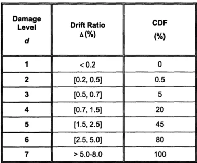
As in [20], the structural and non-structural damage d caused by an earthquake is described using a seven-point scale: d = 1 (no damage), 2 (slight damage), 3 (light), 4 (moderate damage), 5 (heavy damage), 6 (major damage), and 7 (collapse). Each damage level corresponds to a range of the maximum interstory drift ratio A; see Table 1 of [20,

Part II]. Here we use the same drift-ratio intervals (see Table 4.2), except for the collapse state, for which we assume that the minimum drift ratio increases linearly with S, from 5% for S1 to 8% for S8 (high-rises) or S9 (low-rises). The drift ratio of A = 0.7% (damage level d = 4) is also the threshold for structural damage. Lower drift ratios (damage levels d <5 3) involve only non-structural losses.

Table 4.2. Drift ratio and central damage factor (CDF) for different damage levels.

The rate at which each design suffers damage at level d is evaluated using Eq. 3.2, where

y is spectral acceleration at the elastic period of the structure. Erdem Karaca, an MIT

alumnus and now working with the US Geological Survey, provided the hazard and

fragility functions for high-rise and low-rise designs. The methodology adopted to derive

these functions is described henceforth.

The hazard functions H(y) for high-rise and low-rise buildings in Los Angeles,

California, are estimated based on the 2002 USGS national seismic hazard maps and

curves [21] for coordinates - Latitude: 34.05N, Longitude: -118.24W. Since the USGS Damage

Level Drift Ratio CDF

dA(%) (%) 1 < 0.2 0 2 [0.2, 0.5] 0.5 3 [0.5, 0.7] 5 4 [0.7, 1.5] 20 5 [1.5, 2.5] 45 6 [2.5, 5.0] 80 7 > 5.0-8.0 100

hazard maps are available only for a few discrete natural periods, the values at the elastic periods of the structures are obtained through interpolation. For the high-rises we use a second degree polynomial fit (in log-log space) to the USGS hazard data at 0.5, 1.0 and 2.0 seconds, whereas for the low-rises we linearly interpolate the USGS values between 0.3 and 0.5 seconds (again, in log-log space). The hazard curves for spectral acceleration are plotted in Figure 4.1.

(a) High-rises 30

...

...

.; l.-

· · ?·. ..;····... ·...

.1.!

...

.

..

..

..

..

..

...

..

....

...

...

...

...

.

...

.

.

;.

.

..

...

...

.

...

.

.

.

.

.i

i...

.

.

.

.

.

..

.

.

.

..i.

.i

i~

l

...

i...i

...

..

..

.

...

"

".'

...

...

....

"..

"

'

""."

"

...

...

....

..

...

:··

...

·

·

·

·

...

...

...

...

...

·

·

·

··· ···..

..

..

..

...

...

...

....

...

...

I...:...i.

...

.

...

...

..;....

...

...

...

...

...

...

···

····

10

• 10

1

₀₀₂

₁₀₀

Spectral Acceleration, g

(b) Low-rises

Figure 4.1. Spectral acceleration hazard for 8 high-rise and 9 low-rise designs in Los

Angeles, California.

Notice that, since the hazard is expressed here in terms of spectral acceleration, the curves are nearly the same for all the low-rise designs and are more separated for the

high-rise designs. The reverse would be true if we had considered spectral displacement.

The fragility function F(y) for a damage level d gives the probability of exceeding

d as a function of y. We derive this function for each building and each damage state

using time history analysis (THA) of equivalent single-degree-of-freedom (SDOF) models of the structures and the damage drift ratios given above. In THA, we assume

4) ca (.)

x

w

W

10-2

10

₁

₁₀₀

Spectral Acceleration, g

..

...

...

...

...

...

...I.

..

..

;....

.

...

...

....

...

.

hysteretic elastic-perfectly plastic behavior of the SDOF system, with no strength degradation and constant loading and unloading slopes. The required SDOF parameters for the high-rises including the yield strengths and periods are from Tables A.1 and A.4 in Kang [22]. For the low-rises, we assume a linear displacement profile and a yield drift ratio of 1/300 for all the designs. The elastic damping ratio is set to 5%. For the THA of each structure, we use 1585 pairs (EW and NS) of ground motion records from the Next Generation Attenuation ground motion database [23]. The records are from sites with rupture-to-site distance between 10 and 100km and include events with moment magnitudes between M6.0 and M8.0. We do not consider records with closest distances less than 10km to prevent near-source directivity effects and those with distances greater than 100km to reduce computational effort as most of the records in this distance range only resulted in linear response. In addition to the unscaled records, we use records scaled by a factor of 8.0 to increase the number of ground motions that result in nonlinear response.

We apply linear regression in log-log space to the THA results to estimate the mean building response and the variability of the inelastic displacement under given ground motion intensity (i.e. for given elastic spectral acceleration). The conditional inelastic displacement is assumed to follow a lognormal distribution. For the high rises, the (log) response displacement varies linearly with the (log) spectral acceleration and the residual variance may be considered constant; Figure 4.2a illustrates this for different high-rise designs. For the low-rises, this linear homoschedastic model applies only at low ground motion intensities and we fit bilinear models of the type exemplified in Figure 4.2b.

1. Design S1

2. Design _S2

Figure 4.2a. Inelastic spectral displacements from time-history analysis and fitted conditional lognormal parameters (log mean and log mean + one log standard deviation) for high-rise designs [begin].

10: ol C ~ I 1' I 0 ... "~~~n " .. ... ... ... ... ... ... .. . .. .... ... ,i . ...•••, C1 u 10' ~1 ic 0) 'rI, 0

C

10& 10, 10"r ·Ji

M

I._

a

Figure 4.2a. Inelastic spectral displacements from time-history analysis and fitted conditional lognormal parameters (log mean and log mean ± one log standard deviation) for high-rise designs [contd.].

C 0 a,e S10" 1) 10 oj ·O 10>~ tiA

au

5. Design S,

10

!0" 10a 10'" 10" 10'

Spectral Acceleration, g

6. Design S6

Figure 4.2a. Inelastic spectral displacements from time-history analysis and fitted conditional lognormal parameters (log mean and log mean ± one log standard

deviation) for high-rise designs [contd.].

10 2····-·-- ;;·;··· · · -·- -- ·;····;; ; ··· C ~ 47 u"_C 0._ Q10• o _m (0' 41) 0 y0o C A-I 103 102 10' 10C 101 Spectral Acceleration, g E 10 10 10, 5. Design S5 1 0 "j .... ... ... ... .... .... .. ... .... ... ... • .. ... ... .... ... ... ... .. .. ... , ... ... ... ... ... ... ... ... ... .. ... ... ... ... .

102 10 107 10F ' 10 10 Spectral Acceleration, g 7. Design S7 10• 10 E 10 0 10 1C, .1 In_. -. 10 102 10 01 10' Spectral Acceleration, g 8. Design S8

Figure 4.2a. Inelastic spectral displacements from time-history analysis and fitted

conditional lognormal parameters (log mean and log mean ± one log standard

deviation) for high-rise designs [end].

10 -1. . . -10: E10• o 0 c U 50 *1 0 10> 0 C r ·: .i /;" * ,rf 1 r :I i , :: ·i i r · : t I

10 10 100 10 Spectral Acceleration, g 1. Design S1 10,' c 10" Q. I A~ o - 10 U , IA CC 10~ 10'1 100 101 Spectral Acceleration, g 2. Design S2

Figure 4.2b. Inelastic spectral displacements from time-history analysis and fitted conditional lognormal parameters (log mean and log mean + one log standard deviation) for low-rise designs [begin].

10 E 10 10 I-a - 10 0 Ctn -~ "! V' i "I R z ::i i ,I I I

3. Design S₃

4. Design S4

Figure 4.2b. Inelastic spectral displacements from time-history analysis and fitted conditional lognormal parameters (log mean and log mean ± one log standard deviation) for low-rise designs [contd.].

45 ii --P r s I "i ~Y" IE Q 10 0 10 1 10~ 10" 100 10 Spectral Acceleration, g 10 10 10 10 101 ₁₆₀ Spectral Acceleration, g ' - · · ·· ·- · · ·· ·- · ·- ·- ·· · ~ I ·-·--- ··· · · · ·-· ·-··-·-- ·--- ·-·---··-·- ··· · -··· -- ··· ·· · · ···--·- - -- · ·-I : 10 10 '" "··· f i "oil r k·6',~f J!

1 0 g . - ···· ···; ··- ·· · ·- -- ·- · ··· · ·- · ··-- ·--- - ·--- ·· · · · - ·· · ··--- ···- - --. .···· 5. Design S₅ 10t S i. . y _i* ,~ p. 10 10, u10 (/)

,K.

Figure 4.2b. Inelastic spectral displacements from time-history analysis and fitted conditional lognormal parameters (log mean and log mean ± one log standard

deviation) for low-rise designs [contd.].

c mE 1( 0 ,! u•₀ 0 I. U cI, 0 £l I Spectral Acceleration, g i'

7. Design S,

8. _{Design S,}

Figure 4.2b. Inelastic spectral displacements from time-history analysis and fitted conditional lognormal parameters (log mean and log mean + one log standard deviation) for low-rise designs [contd.].

10 --10 u - io C 10'1 ₁₀0 ₀₁ Spectral Acceleration, g 10 0, 10 10₁₀, .i 1101 10 101 Spectral Acceleration, g 10,2

9. Design S9

Figure 4.2b. Inelastic spectral displacements from time-history analysis and fitted conditional lognormal parameters (log mean and log mean + one log standard deviation) for low-rise designs [end].

For each structure, the drift ratio thresholds for the various damage states are converted to

inelastic spectral displacements for the equivalent SDOF model. For the high-rises, the

conversion accounts for the bias in estimating the maximum interstory drift ratio from the maximum roof displacement. For this purpose we use the bias factors (and their standard

deviations) given in [24]. The same factors were used by Kang [22]. For the low-rises, a

linear displacement profile with height is assumed and no bias factor is applied.

Using the regression results illustrated in Figure 4.2 and the damage thresholds

for the inelastic drift ratio, we obtain the fragility curves, which give the probability that

each building exceeds various levels of damage as a function of ground motion intensity. The fragility curves for high-rise and low-rise designs are given in Figure 4.3a and Figure 4.3b respectively, they give probability of exceeding different damage levels (which are

1O2 -- 1~ · .·.--... · · - --- · ·. · - --.. ·..-C - · 4· C CI0

r=

a.

defined in Table 4.2) as a function of spectral acceleration. From Figure 4.3a-1 we see that at spectral acceleration of 0.1 g, the high-rise design S1 exceeds moderate and heavy damage with a probability of 0.7 and 0.1 respectively or we can say that at a spectral

acceleration of 0.1 g the probability of suffering moderate damage is 0.6.

Due to the different regression models for high- and low-rises shown in Figure 4.2, the fragility curves have the shape of lognormal distributions for the high-rises and more complicated shapes for the low-rises.

1. Design St

Figure 4.3a. Fragility curves for different damage states for high-rise designs [begin].

10_! SO..g2 _----7, -0.4f 0, 1/ 101 10, 10' Spectral Aceleratlon, g = 10,2 7r~~~ ..i ·! -1 1

U

i

/ "

/

•

A

Figure 4.3a. Fragility curves for different damage states for high-rise designs [contd.].

10 ' -. - Slight 0 I'

0 0

f

I

i

I

iI ,

I it t1

i i

c

.·C

4. Design S₄

5. Design S5

Figure 4.3a. Fragility curves for different damage states for high-rise designs [contd.].

so

a0.

0.8 0.7 ompte i 06-05! 0.4 i

0.31

0.2

ii

iI

Figure 4.3a. Fragility curves for different damage states for high-rise designs [contd.].

45

,1~

10

.-- Moderate * 07 6-compi

OV

0,31

011

/

,ii

l

-

r

..

'2

...

:

__

_J

.

Figure 4.3a. Fragility curves for different damage states for high-rise designs [end].

1. Design SI

Figure 4.3b. Fragility curves for different damage states for low-rise designs [begin].

0.9

1C

)I

2. Design S2

0.7[

0.

4

0i

Figure 4.3b. Fragility curves for different damage states for low-rise designs [contd].

0. 0 20. L

0.o

4

Spectral Acceleration, g

4. Design S4

5. Design S,

Figure 4.3b. Fragility curves for different damage states for low-rise designs [contd].

0.9

o6!

S03i

I

6. Design S6

7. Design S7

Figure 4.3b. Fragility curves for different damage states for low-rise designs [contd].

0. 1 -. - Slight O.9 -- -U _Modemlatetv PAWr 0.7-CompeI 0.5

1

0-.4i

0.

9

H---

UOM

o

0.5

/f !

i

Figure 4.3b. Fragility curves for different damage states for low-rise designs [end].

!I r • -•-? 2£.7,.s :• 0.

go.

0o.

The functions H(y) and F(y) derived from this analysis are taken as the expected hazard and fragility functions at the time of construction and are used in Eq. 3.2 to calculate the rate at which each design suffers different damage levels d. These damage rates are listed in Tables 4.3 and 4.4. The last column of these tables gives the frequency ratio Fs, which is used to track the structural state of the building, it is described in detail in the next

section.

Design _{Damage Level d}

Level Fs Ratio

S 1 2 3 4 5 6 7

1 0.0172 0.0597 1.00E-02 1.03E-02 2.16E-03 5.64E-04 9.82E-06 1

2 0.0281 0.0522 8.52E-03 9.08E-03 1.69E-03 3.87E-04 5.52E-06 101/4

3 0.0362 0.0470 7.29E-03 7.95E-03 1.26E-03 2.82E-04 3.11E-06 102/4 4 0.0408 0.0438 6.87E-03 7.29E-03 1.04E-03 2.26E-04 1.75E-06 103/4

5 0.0441 0.0412 6.69E-03 6.90E-03 9.18E-04 1.94E-04 9.82E-07 10

6 0.0504 0.0369 6.18E-03 5.75E-03 7.02E-04 1.41E-04 5.52E-07 10_5/4

7 0.0539 0.0346 5.85E-03 4.95E-03 5.76E-04 1.14E-04 3.11E-07 106/4

8 0.0564 0.0329 5.55E-03 4.51E-03 5.30E-04 1.10E-04 9.82E-08 100

Table 4.3. Damage rates (events/year) for high-rise designs in Los Angeles, California.

Design _{Damage Level d}

Level Fs Ratio

S 1 2 3 4 5 6 7

1 0.8370 0.0193 1.21E-03 1.19E-03 2.91E-04 1.32E-04 2.73E-05 1

2 0.8523 0.0155 1.07E-03 1.06E-03 2.65E-04 1.17E-04 1.54E-05 101/ 4

3 0.8683 0.0118 9.04E-04 8.85E-04 2.11E-04 8.02E-05 8.64E-06 102/4 4 0.8843 0.0090 7.48E-04 7.68E-04 1.59E-04 5.71E-05 4.86E-06 103/4

5 0.8440 0.0067 6.02E-04 6.55E-04 1.05E-04 3.82E-05 2.73E-06 10 6 0.8505 0.0050 5.08E-04 4.30E-04 6.00E-05 2.20E-05 8.64E-07 106/4

7 0.8567 0.0038 3.68E-04 2.36E-04 3.44E-05 1.08E-05 1.54E-07 109/4

8 0.8631 0.0028 1.87E-04 1.28E-04 1.79E-05 4.36E-06 2.73E-08 1000

9 0.8696 0.0019 9.95E-05 7.10E-05 7.72E-06 1.33E-06 2.73E-09 10,000

For low-rises, as we go from S=I to S=9, the period of the designs reduces by a factor of 0.5 and the rate of getting into d=6 (heavy damage) reduces by a factor of 100. As we go from S=1 to S=8 designs in high-rises the period changes by a factor of one-half, but the rate of getting into d=6 reduces only by a factor of 5. For the high-rises, the damage rates are insensitive to the seismic design S, for all the damage levels, except for the collapse state (d=7). This is because for structures with long natural periods the peak interstory drift is controlled by the peak ground displacement, with only a small dependence on building stiffness. The drift ratio threshold for collapse state is taken to increase linearly with S and so we observe that for high-rises the rate of collapse is sensitive to S.

4.2 Repair/ Retrofitting Strategies and Frequency Ratios

Earthquake-induced damage involving structural damages (d > 4) necessitates the repair of the building to the strength of one of the initial designs. The building could be repaired back to the pre-earthquake conditions or structurally upgraded. Changes in E and R (see

Section 3.3) could cause the building to violate the regulatory constraints, requiring retrofitting action. In the base case, we consider repairing back to the pre-earthquake structural state, but if E and R change such that one needs to retrofit, then retrofitting is done to the lowest admissible strength consistent with the values of E and R. Other repair and retrofit strategies are considered in Chapter 5.

As mentioned in Section 3.1, these changes in structural state, epistemic uncertainty and the regulatory limits are tracked by three state variables and the integer levels of the state variables S, E and R for high-rise and low-rise designs correspond to