Deformation Correction in Ultrasound Imaging
in an Elastography Framework
MASSA04S
by04
Shih-Yu Sun
LIBRARIES
B.S. Electrical Engineering, National Taiwan University (2006)
ARCHIVES
Submitted to the Department of Electrical Engineering and Computer Science
in partial fulfillment of the requirements for the degree of
Master of Science in Electrical Engineering and Computer Science
at the
MASSACHUSETTS INSTITUTE OF TECHNOLOGY
September 2010
0 Massachusetts Institute of Technology 2010. All rights reserved.
A uthor...
Department of Electrical Engineering and Computer Science
August 27, 2010
Certified by ...
. .
...
...
Research Scientist, Department of Mechanical Engineering
Thesis Supervisor
A -~
Accepted by...
...
T
Terry P. Orlando
Chair, Department Committee on Graduate Students
Deformation Correction in Ultrasound Imaging
in an Elastography Framework
by
Shih-Yu Sun
Submitted to the Department of Electrical Engineering and Computer Science
on August 27, 2010, in partial fulfillment of the
requirements for the degree of
Master of Science in Electrical Engineering and Computer Science
Abstract
Tissue deformation in ultrasound imaging is an inevitable phenomenon and poses challenges to the development of many techniques related to ultrasound image registration, including multimodal image fusion, freehand three-dimensional ultrasound, and quantitative measurement of tissue geometry. In this thesis, a novel trajectory-based method to correct tissue deformation in ultrasound B-mode imaging and elastography is developed in the framework of elastography.
To characterize the change of tissue deformation with contact force, a force sensor is used to provide contact force measurement. Correlation-based displacement estimation techniques are applied to ultrasound images acquired under different contact forces. Based on the estimation results, a two-dimensional trajectory field is constructed, where pixel coordinates in each scan are plotted against the corresponding contact force. Interpolation or extrapolation by polynomial curve fitting is then applied to each trajectory to estimate the image under a specified contact force.
The performance of displacement estimation and polynomial curve fitting are analyzed in a simulation framework incorporating FEM and ultrasound simulation. Influences of parameter selection are also examined. It is found that in displacement estimation, the coarse-to-fine approach outperforms single-level template search, and correlation filtering in coarse scale provides noticeable improvement in estimation performance. The strategies of image acquisition and order selection in polynomial curve fitting are also evaluated. Additionally, a finer force resolution is found to give better performance in predicting pixel positions under zero force.
Deformation correction in both B-mode imaging and elastography is demonstrated through simulation and in-vitro experiments. The performance of correction is quantified by translational offset and area estimation of the tissue inclusions. It is found that, for both B-mode and elastography images, those performance metrics are significantly improved after correction. Moreover, it is shown that a finer resolution in force control gives better performance in deformation correction, which agrees with the analysis of polynomial curve fitting.
Thesis Supervisor: Brian W. Anthony
Acknowledgements
I would like to thank my advisor, Dr. Brian Anthony, for his guidance. Brian always gives inspiring advices in conducting the research and shows great patience during discussion. I learn a lot more than doing research from working with him.
I would also like to thank Matthew Gilbertson. His awesome probe system has
enabled me to test various ideas and validate the proposed method. I am often amazed
by Matthew's skills in mechanical design and machining. I believe he can make
anything with a block of metal.
Last but not least, I would like to thank my parents Kao-Chin Sun and Shu-Huei Chen, my sisters Yi-Chun and Yu-Ting for being extremely supportive to me. And thank you, Yi-Ping. Your unconditional friendship, company, and love have been, and will always be, invaluable to my life.
Contents
1 Introduction
15
1.1 Related W ork ... 16 1.2 Contributions... 17 1.3 Thesis Outline ... 172
Background
19
2.1 Ultrasound B-mode Imaging...192.2 Ultrasound Elastography... 20
2.3 Summary... 24
3 Trajectory-Based Deformation Estimation and Correction
25
3.1 Concept ... 253.2 Two-Dimensional Displacement Estimation ... 27
3.2.1 Correlation-Based Template Matching ... 28
3.2.2 Coarse-to-Fine Search ... 30
3.2.3 Correlation Filtering ... 30
3.2.4 Subsample Estimation ... 33
3.2.5 Smoothing with Non-Uniform Spatial Resolution ... 35
3.3 Polynomial Curve Fitting... 37
3.4 Summary... 37
4 Ultrasound Simulation Using Finite-Element Methods
39
4.1 Simulation Setup... 394.1.1 FEM ... 39
4.1.2 Field II... 41
4.2 Displacement Estimation ... 42
4.2.1 Single-Level and Coarse-to-Fine Search... 42
4.2.2 Analysis of Parameter Selection... 47
4.3 Curve Fitting ... 50
4.3.1 Noise Modeling in Displacement Estimation...51
4.3.2 Analysis of Parameter Selection... 53
4.4 Deformation Estimation and Correction...55
4.4.1 Deformation Correction with 1 OOmN Force Resolution ... 56
4.4.2 Comparison of Force Resolutions ... 60
4.5 Sum m ary ... 62
5 In-Vitro Experiments
65
5.1 Experim ent Setup... 655.1.1 Force-Controlled Ultrasound Probe... 66
5.1.2 Ultrasound Imaging System ... 68
5.2 Experiment Results and Discussion...69
... 72.6 5.3 Sum m ary ... 72
6 Conclusions
73
6.1 Sum m ary ... 7 3 6.2 Future W ork ... 74Bibliography
77
8List of Figures
1-1 The ultrasound images of brachial artery under varying levels of probe
com pression... 15
2-1 Only envelopes of the reflected signal are used for B-mode image
formation, but additional information about the phase is inherent in the R F data. ... . 20
2-2 Illustration of strain estimation: in (a), a definition of strain is given; in
(b), the same concept is applied on a displacement field...22
2-3 The simulated pre-compression and post-compression B-mode images. ...23
2-4 The displacement estimation results (a) and the corresponding strain image (b) in the simulated ultrasound elastography...23
3-1 The B-mode image of a homogeneous tissue under compression and the
corresponding displacement field... 26
3-2 Behaviors of tissue deformation under varying contact forces could be
characterized by tracking pixel movements along the ultrasound image sequence ... 26 3-3 The image under a specified contact force could be estimated from the
trajectory field, which describes pixel movement with changing contact forces. ... . . 27
3-4 An overview of the 2D displacement estimation method ... 28
3-5 Displacement estimation is performed based on a template-matching
scheme using the waveforms inherent in the ultrasound images ... 29
3-6 Illustration of the correlation filtering method... 31
3-7 Illustration of coarse-scale displacement estimation...32
3-8 Design of the fine-scale search region to reduce possible peak detection
errors brought by correlation filtering ... 33
3-9 Curve fitting using three sample points is applied in two directions for
subsample accuracy in displacement estimation...34
3-10 (a) simulated axial displacement estimation results; (b) the black dots 9
indicate the occurrence of peak-hopping errors in the estimation results ... 36 3-11 (a) computed correlation coefficients in axial displacement estimation;
(b) the black dots indicate the locations where the correlation
coefficients are lower than 0.5 ... 36
4-1 The setup in FEM ... 40
4-2 A sampled set of the scatterers in ultrasound simulation ... 42
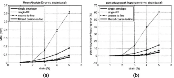
4-3 The axial displacement estimation MAE (a) and peak-hopping errors (b)
versus the applied strain ... 45
4-4 The axial displacement estimation MAE (a) and peak-hopping errors (b)
versus the probe elevational offset ... 45
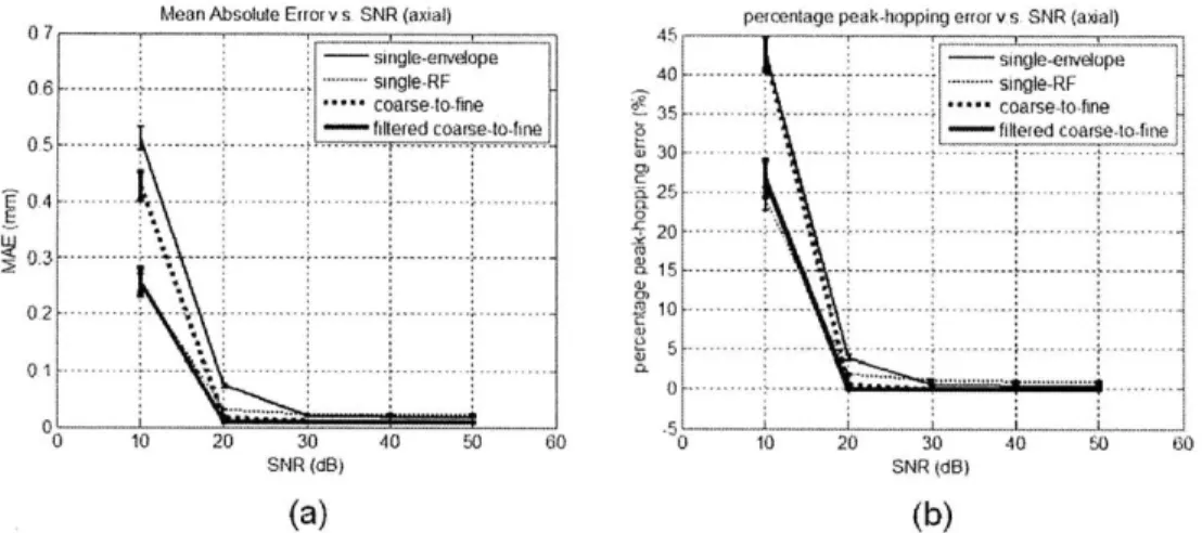
4-5 The axial displacement estimation MAE (a) and peak-hopping errors (b)
versus SN R ... 46 4-6 The lateral displacement estimation MAE versus the strain (a),
elevational offset (b), and SNR (c)...47 4-7 The axial displacement estimation MAE (a) and peak-hopping errors (b)
versus the coarse-scale kernel length ... 48
4-8 The axial displacement estimation MAE (a) and peak-hopping errors (b)
versus the fine-scale kernel length ... 49
4-9 The axial displacement estimation MAE (a) and peak-hopping errors (b)
versus the coarse-scale correlation filter length ... 50
4-10 The lateral displacement estimation MAE versus the coarse-scale kernel length (a), the fine-scale kernel length (b), and the coarse-scale filter length (c)... 50 4-11 Selected strain-force points for varying force resolutions: 20mN, 50mN,
and 1OOm N ... 52
4-12 Illustration of displacement error induced by noise in force control ... 53 4-13 Projection MAE versus the polynomial order: eight frames with a
1 OOm N resolution ... 54
4-14 Projection performance versus the number of frames used for varying force resolutions ... 55 4-15 The B-mode image of the 300 mN-compressed inclusion (a) is
corrected (b). From the comparison between (a), (b) and the true
uncompressed inclusion contour (c), it is shown that the deviation in the
position of the inclusion can be remedied. (d) ... 57
4-16 The performance of deformation correction is quantified by three parameters that are derived from area estimation. They are true positive (TP), false positive (FP), and false negative (FN)...58
4-17 The elastography image under 200-300 mN compression (a) is corrected (b). From the comparison between (a), (b) and the true uncompressed inclusion contour (c), it is shown that the deviation in the position of the inclusion can be remedied. (d)...59
4-18 Deformation correction of B-mode images: compare 20 mN, 50 iN, and 100 m N force resolution... 60
4-19 Difference images between the corrected B-mode images and the true uncompressed image using 20 mN, 50 mN, and 100 mN force resolution ... 61
4-20 Deformation correction of elastography: compare 20 mN, 50 mN, and 100 m N force resolution... 62
5-1 The breast ultrasound needle biopsy phantom used in the in-vitro experiment (from http://www.cirsinc.com/)...65
5-2 The in-vitro experim ent setup ... 66
5-3 The force-controlled ultrasound probe ... 67
5-4 GUI of the force-controlled probe... 67
5-5 GUI of the ultrasound imaging system...68
5-6 The B-mode image of the 4 N-compressed inclusion (a) is corrected to 1 N compression (b). From the comparison between (a), (b) and the true 1 N-compressed inclusion contour (c), it is shown that the deviation in the shape and position of the inclusion can be remedied. (d) ... 70
5-7 The elastography image under 3.5-4 N compression (a) is corrected to 1 N compression (b). From the comparison between (a), (b) and the true 1 N-compressed inclusion contour (c), it is shown that the deviation in the position of the inclusion can be remedied. (d)...71
List of Tables
4-1 The hyperelastic parameters of normal and pathological breast tissue in
F E M ... . . 4 1
4-2 Parameters for the search schemes ... 43
4-3 The efficient orders for each pair of force resolution and number of fram es ... . . 54
4-4 The most efficient number of frames and the corresponding efficient
order for each force resolution ... 55
4-5 Performance of correcting the B-mode image contour under 300 mN compression as measured by the translational offset from the true
uncompressed contour and the area estimation parameters ... 58
4-6 Performance of correcting the elastography image contour under
200-300 mN compression as measured by the translational offset from
the true uncompressed contour and the area estimation parameters ... 59
4-7 Performance of correcting the B-mode image contour under lOOmN compression using 20 mN, 50 mN, and 100 mN force resolution as measured by the translational offset from the true uncompressed
contour and the area estimation parameters ... 61
4-8 Performance of correcting the elastography image contour under 100-(120 mN, 150 mN, 200 mN) compression using 20 inN, 50 mN, and 100 mN force resolution as measured by the translational offset from the true uncompressed B-mode image contour and the area
estim ation param eters... 62
5-1 Performance of correcting the 4 N-compressed B-mode image contour
to 1 N compression as measured by the translational offset from the true
1 N-compressed contour and the area estimation parameters ... 70
5-2 Performance of correcting the elastography image contour under 3.5-4
N compression to 1 N compression as measured by the translational
offset from the true 1 N-compressed B-mode image contour and the
area estim ation param eters... 71
Chapter 1
Introduction
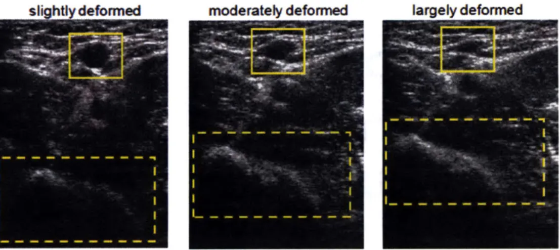
Diagnostic ultrasound imaging technology is indispensable nowadays as it provides inexpensive and non-invasive real-time imaging with high spatial resolution. Ultrasound imaging is typically performed in a manner where a probe makes firm contact with the skin for good image quality. In this procedure, deformation of the underlying tissue is inevitable, and thus structures shown in imaging are distorted. This phenomenon is shown in Figure 1-1, where the appearance of the same tissue changes due to varying levels of probe compression. The blob of tissue enclosed by dashed lines undergoes translational offset, and the cross-sectional area of the brachial artery (enclosed by solid lines) shrinks with an increased compression level.
Figure 1-1 The ultrasound images of brachial artery under compression
varying levels of probe
In most cases, this distortion effect does not impede diagnosis, since most of the characteristics of tissue are retained under compression. In fact, tracking pixel displacements in a sequence of compressed tissue images provides information to discriminate between normal and pathological tissue in elastography. [1] However, for applications where the undeformed appearance of biological tissue is required,
avoiding or correcting tissue deformation becomes crucial. For example, in freehand three-dimensional ultrasound (freehand 3D US), where the shape of tissue is reconstructed by stacking two-dimensional (2D) slices acquired in varying probe positions and contact forces, the corresponding pixels can be accurately aligned only if the deformation patterns in each slice can be appropriately corrected. Furthermore, deformation correction applied in 3D US facilitates quantitative measurement of tissue volumes and analysis of the shape. [2] The need to correct deformation also arises in multimodal image processing, in which tissue deformation in ultrasound scanning has to be corrected before the image can be accurately registered with those from other imaging modalities, such as X-ray, optical coherence tomography (OCT), computed tomography (CT), and magnetic resonance imaging (MRI). Other applications that could potentially benefit from the deformation correction method include computational anatomy and image-guided surgery [3],[4].
1.1 Related Work
Several deformation correction methods have been proposed, aiming to estimate B-mode images that would have been acquired in ultrasound scanning as if there had been no probe contact. In the surface model method proposed by Burcher et al. [2], the compression level of each scan frame are estimated using probe contact force measurement. Inter-frame registration is achieved, but this method does not address in-plane deformation of the underlying tissue. In [5], Treece et al. proposed a method that is able to correct in-plane deformation along the axial direction, which is the most significant effect due to probe compression. This method estimates tissue deformation
by combining probe position measurement and image-based registration. However, the
method becomes inadequate when it is important to characterize tissue deformation in two or three dimensions. Also, in this method, tissue elasticity is assumed to be uniform over the whole region of interest, but it is rarely the case in biological tissue.
A method that takes into account two-dimensional pixel movement was proposed by Burcher et al. [2], where tissue deformation patterns are predicted based on contact
force measurement and finite-element modeling. Correction of deformation is performed by an inverse approach. Nevertheless, this method incorporates a priori
knowledge of the spatial variation of tissue elasticity, which can be hard to measure in clinical settings.
To reduce dependence on assumptions of tissue elastic property, a preliminary study of trajectory-based deformation correction is described in the work of Burcher [6]. In this method, pixel trajectories under varying compression levels are estimated by B-mode speckle tracking. [7] Linear polynomial functions are then used to fit the trajectories to predict tissue geometry under a specified compression level. Encouraging in-vivo results of inclusion contour prediction are presented. However, this method models the mechanical behaviors of biological tissue deformation by linear dynamics. This approximation is applicable only when the range of applied contact forces is small.
1.2 Contributions
In this thesis, a novel deformation correction method developed within the framework of ultrasound elastography is described. This method allows integration with the existing elastography technique and requires no additional operator effort in the workflow. The contributions include:
e A novel application of elastography to solve the deformation correction problem in
ultrasound imaging.
- The ability of this method to correct tissue deformation when the range of applied contact forces is large
- Extension of deformation correction methods to addressing tissue deformation in ultrasound elastography
e An ultrasound simulation platform incorporating FEM and Field II for the
verification of algorithms involving imaging of biological tissue in varying compression states
1.3 Thesis Outline
The remainder of this thesis is organized as follows. In Chapter 2, current technologies in ultrasound imaging are briefly introduced, including B-mode imaging and
elastography. Chapter 3 describes the concept of the proposed trajectory-based deformation correction method and details of the algorithm. This method is validated
by simulation and in-vitro experiments, which are presented in Chapter 4 and Chapter 5,
respectively. This thesis concludes in Chapter 6 with a summary of the above chapters and a discussion of future work for possible improvement and extension of the proposed method.
Chapter 2
Background
The deformation correction method proposed in this thesis is developed within the framework of ultrasound elastography and is applicable to both ultrasound B-mode images and elastography. This chapter provides an introduction to the existing technologies related to this method. Section 2.1 describes the physics and process of B-mode image formation. Section 2.2 presents the method to perform ultrasound elastography using probe compression.
2.1 Ultrasound B-mode Imaging
Ultrasound imaging is an indispensable diagnosis tool due to its low cost and real-time nature, and has been under active development for decades. This technology uses mechanical waves modulated by a carrier frequency of higher than 20kHz to interrogate the structures of the underlying tissue. The wave is generated from electrical excitation of a piezoelectric transducer and propagates through the human body via a layer of transmission gel. The transmitted wave is reflected in human body when interfaces of mismatched acoustic impedance are encountered. Therefore, the reflected waveform is determined by the spatial variation in acoustic impedance of tissue and sensed by the same transducer. Envelope detection is then performed on the received radio-frequency (RF) wave, as illustrated in Figure 2-1. After repeating this procedure at preprogrammed positions, the acquired envelopes are post-processed and aligned to form a brightness image, or B-mode image, that describes the tissue structure. Examples of B-mode images can be seen in Figure 1-1.
Conventionally, three specific terminologies are used to refer to the directions in ultrasound scanning; they are axial, lateral, and elevational directions. Axial and lateral directions refer to the two dimensions that define the scan plane, with axial direction being parallel to ultrasound beam propagation. Elevational direction is orthogonal to the scan plane.
It should be emphasized that although only envelopes of the reflected waves are used to form a B-mode image, the raw RF data provide additional information about the phase of wave propagation, which is often useful for purposes other than image formation. In Chapter 3, both the use of RF data and the envelopes for pixel displacement estimation are discussed. The performances are analyzed in Chapter 4.
B-mode image
RF data
Figure 2-1 Only envelopes of the reflected signal are used for B-mode image formation, but additional information about the phase is inherent in the RF data.
2.2 Ultrasound Elastography
Spatial variation of brightness in B-mode images can describe the structure of tissue under the assumption that the acoustic impedance varies noticeably in different types of tissue. However, this assumption does not always hold. There are times when pathological tissue is not discernible from the surroundings in B-mode images. As a result, imaging methods that can detect tissue properties other than acoustic impedance are often desired.
Palpation has long been an effective method for diagnosis of pathologies. It is based on the fact that pathological tissue normally has higher stiffness than the surroundings. This observation implies that the ability to detect spatial variation in tissue stiffness could potentially assist diagnosis. One of the most popular methods for detecting this variation involves exerting a sequence of compression with an ultrasound probe on the tissue, imitating the practice of palpation, and acquiring images at the same time. Stiffness at each point of the tissue is then differentiated by tracking pixel displacements in the acquired images.
In solid mechanics, stiffness is often characterized by Young's modulus, which is defined as the ratio between stress and the induced strain at a particular point. Normally, to detect tissue abnormality in ultrasound images, strain is estimated instead of the Young's modulus. This simplification is based on the assumption that the stress field is uniform over the region of interest.
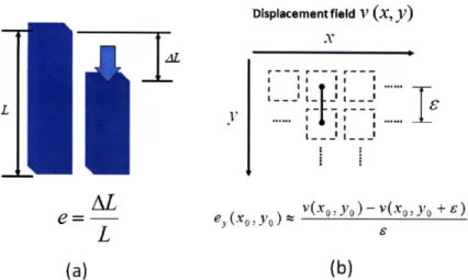
The definition and estimation of strain in elastography are illustrated in Figure 2-2. Suppose a rod with length L is squeezed by AL under a certain compression, as shown in Figure 2-2(a). The induced strain e is defined as
AL
e = - (2.1)
L
The same concept can be applied to estimating strain from the displacement field in Figure 2-2(b). It can be imagined that, when there is no compression, a tiny rod with
length s lies between (xo, yo) and (xo, yo + E), where , is the distance between
neighboring pixels. Under the compression, the spatial distribution of displacements in
y (the axial direction), v(x, y), can be measured. Note that since the tissue is seen with
respect to the coordinate system attached to the probe, points of the tissue in the image appear to be moving upward during compression.
Under the compression, the strain in y at the position (xo, yo), ey (xo, yo), can be
approximated as v(xo, Yo) - v(xo, yo + e), the change in length of the rod, divided by
the original length &. Note that to observe only the variation in strain instead of the exact values, the division by P can be omitted since it is a constant over the field.
Therefore, in the implementation of strain imaging, only the term v(xO, Yo)
Displacement field V
(X,
y)
LI
_AL
_ _ _ _ _(a)
(b)
Figure 2-2 Illustration of strain estimation: in (a), a definition of strain is given; in (b),
the same concept is applied on a displacement field.
It should be emphasized that, in ultrasound image formation, the spatial sampling distance in the axial direction is determined by the temporal frequency with which reflected ultrasound waves are sampled, whereas the sampling distance in the lateral direction is determined by the element width of the probe array. Therefore, the spatial resolution in the axial direction is much higher than that in the lateral direction. For the configuration of the Terason t3000 imaging system, for instance, the spatial sampling
distance is about 26
sm
axially and 150 gm laterally. [8] As a result, strain estimation isnormally applied only in the axial direction for elastography, although the performance could be improved by incorporating estimation of lateral strain. [9]
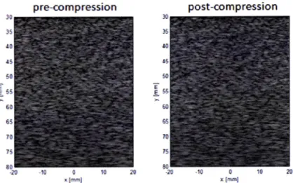
In the following, a simulated example of ultrasound elastography is described to demonstrate the feasibility of detecting pathological tissue in elastography even if it is invisible in B-mode images (see Chapter 4 for the simulation framework.) A pre-compression and a post-compression B-mode image of a tissue phantom are shown in Figure 2-3. The elasticity in a circular region of the phantom is set to be higher than the surroundings to mimic pathological tissue, but the spatial distribution of acoustic impedance is set to be uniform over the whole field. As a result, the simulated pathological tissue region is not observable in the B-mode images.
pre-compression
post-compression
35 3 a0 40 *$ 4 50 50 60 60 65 65 70 70 75 75 -20 -10 0 10 20 20 -10 0 10 20 xIMi1 x (miFigure 2-3 The simulated pre-compression and post-compression B-mode images.
The results of displacement estimation in y are shown in Figure 2-4 (a) (see Chapter 3 for the displacement estimation algorithm.) By applying the strain estimator on the displacement field, the strain image is acquired as in Figure 2-4 (b). In the strain image, it is obvious that there is a nearly circular inclusion with less strain, which implies higher stiffness in the region under the assumption of uniform stress. This observation agrees with the simulation setup of tissue elasticity properties.
dsolacment estmaon in v strain imaire
0-02 755 -. 66
~
-07 6 4870 -75 75 4M 5 _1 1 _5 15 fwn 15 AD -5 0 5 10 15~~?if,"
fTW1 vT(a)
(b)
Figure 2-4 The displacement estimation results (a) and the corresponding strain image
(b) in the simulated ultrasound elastography
2.3 Summary
This chapter provided a brief introduction to ultrasound B-mode imaging and elastography. B-mode images are formed by aligning the envelopes of the received RF data. Estimation of the displacement field due to probe compression can be performed on either the RF data or the envelopes. Elastography is performed in the form of strain imaging using the displacement estimates. Through simulation, it has been shown that elastography can show pathological tissue even when it is invisible in B-mode imaging.
Chapter 3
Trajectory-Based Deformation
Estimation and Correction
In this thesis, the trajectory-based deformation estimation and correction method is proposed to estimate the ultrasound B-mode and elastography images under a specified compression level, in which zero compression is of particular interest. The method involves modeling tissue deformation using pixel displacement fields and performing extrapolation or interpolation in the fields. In this chapter, this procedure is described in detail. Section 3.1 presents the high-level concept of the method. Section 3.2 covers the design of a two-dimensional displacement estimation algorithm. Section 3.3 describes the application of polynomial curve fitting to the estimated displacement fields to perform extrapolation.
3.1 Concept
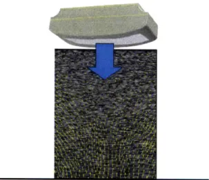
The trajectory-based deformation estimation and correction method is an extension to the elastography technique. As described in Section 2.2, elastography uses a sequence of compressed tissue images and the corresponding displacement estimates to differentiate elasticity of the underlying tissue. Actually, these displacement estimates could also be used to model tissue deformation between the compression states. Figure
3-1 gives an example of the displacement field of a homogeneous tissue under
compression.
To characterize the force-varying deformation patterns of the biological tissue under investigation, a sequence of ultrasound images under different contact forces are acquired, and the corresponding forces are measured by a force sensor installed in the probe. A set of displacement fields is established by tracking each pixel over the whole field of view along the image sequence, as shown in Figure 3-2. Here tissue
deformation in the elevational direction is assumed to be negligible and is ignored in displacement estimation.
Figure 3-1 The B-mode image of a homogeneous tissue under compression and the corresponding displacement field
contact force axial lateral ultrasound image tracking pixels I iI
Figure 3-2 Behaviors of tissue deformation under varying contact forces could be characterized by tracking pixel movements along the ultrasound image sequence
Knowledge of contact forces and the pixel displacement fields allow the construction of a trajectory field for the specific subject, in which pixel coordinates in the scan planes are plotted against the corresponding contact forces, as shown in Figure
3-3. Pixel positions under a specified contact force are then estimated from the
trajectories. Specifically, the locations of pixels under a specified contact force within
26
NOMPMMM"-the acquired force range could be estimated from linear interpolation between two neighboring forces. The images under contact forces beyond the acquired force range could be estimated by extrapolation. One selection of particular interest is zero force, which provides an estimate of the image that would have been acquired if there had been no contact force.
contact force
0
Figure 3-3 The image under a specified contact force could be estimated from the trajectory field, which describes pixel movement with changing contact forces.
3.2 Two-Dimensional Displacement Estimation
Displacement estimation is crucial in characterizing the force-varying tissue deformation patterns and is pivotal to the performance of the deformation correction method. Several methods have been developed to estimate pixel displacements in ultrasound images in both the axial and lateral direction, including B-mode block-matching [7],[10], phase-based estimation [11], RF speckle tracking [9],[12-15], and incompressibility-based methods [16],[17]. Those methods all pose displacement estimation as a time-delay problem, which has been extensively studied in the literature.
[18]
In this thesis, a 2D displacement estimation algorithm is developed based on an iterative ID displacement estimation scheme, where lateral displacement estimation is performed at the locations previously found in the corresponding axial estimation. [19] Coarse-to-fine template-matching is performed axially, with normalized correlation ...
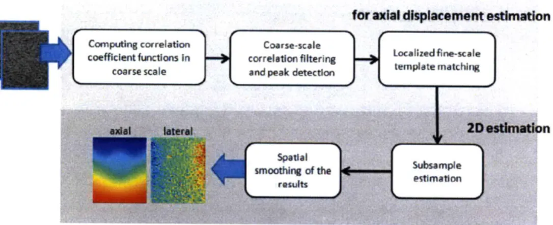
coefficients as a similarity measure. Subsample estimation accuracy is achieved by curve fitting. [20] This estimation algorithm is summarized in Figure 3-4, and the essential steps are detailed in the following subsections.
for axl displacement estmation
Computing correlation
Coarse-scale
coefficient functions In correlation filtering eoad m ae thdinc
coarse scale and peak detection temethin
Subsample
estimation
Figure 3-4 An overview of the 2D displacement estimation method
3.2.1 Correlation-Based Template Matching
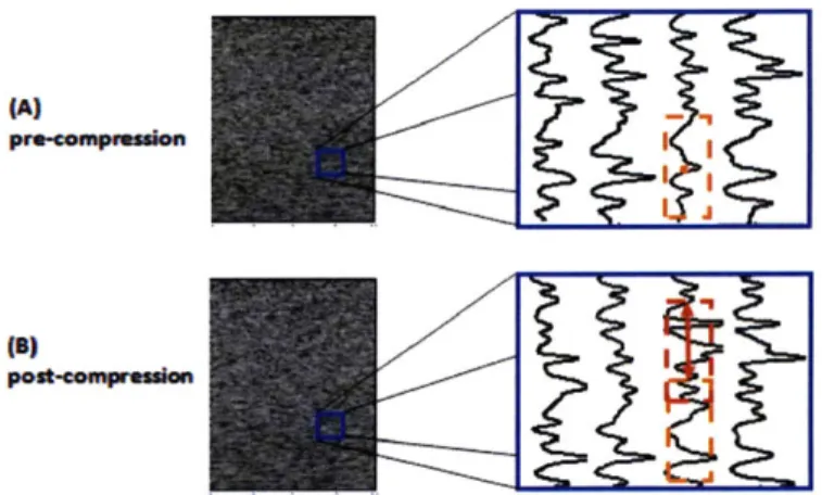
Template matching is one of the most frequently used methods in motion estimation. Figure 3-5 gives an example to illustrate the matching method in the axial
direction, in which the displacement field is to be estimated between pre-compression
(A) and post-compression (B) states. Suppose in image A, displacement of the location
indicated by the orange dot is to be measured. A kernel centered at that point is defined to include the pre-compression segment sA(t), which is to be searched in image B. The search starts from the corresponding location in image B and moves along the
post-compression waveform sB(t) to find the best match of the pre-compression segment. In a similar manner, all of the waveforms in image A are axially divided into overlapping kernels, and each of the segments is compared with the corresponding waveforms in image B.
#At
(9)
Figure 3-5 Displacement estimation is performed based on a template-matching scheme using the waveforms inherent in the ultrasound images
Among other frequently used similarity measures like MAE (Mean Absolute Error) and MSE (Mean Squared Error), the normalized cross correlation coefficient function p(t, t + T) is used here, which is defined by
f+T (sA( -r) - pA)(sB(V) - pa)dp
p(t, t + ) = - , (3.1)
GAGB
where t denotes the point of estimation in the axial direction and r denotes the lag of the correlation coefficient function. Here T denotes the time span of the correlation
kernel. pA and pB are the mean values of sA(t) and sB(t), respectively. GA and GB
are the standard deviations. After p(t, t + r) is estimated, peak detection is performed on this function. The lag that gives the peak is considered the location corresponding to
the best match. Note that only the sampled version of p(t, t + T) is acquired, so
interpolation is performed to find the peak of p(t, t + r) and the corresponding lag. (See Section 3.2.4 for the interpolation method)
Note that here displacement estimation in tissue compression is approximated as a time-delay problem, in which there is assumed to be no intra-kernel deformation. However, when the chosen kernel length T is relatively large under the applied strain, this approximation error becomes noticeable, and as a result, the location of correlation peak might deviate from the true displacement value. On the other hand, increasing the number of samples in correlation estimation could reduce the variance of estimation
.... ... .. .... ... .
- '.'.j'N"! '- .j. :::::: W ::: :::::: ::: ...
error. Therefore, in determining the kernel length T, one should consider the tradeoff between minimization of the mean and the variance of correlation estimation error.
In addition to estimation accuracy, the dynamic range of the algorithm should also fulfill the need of the specific application. The range is significantly influenced by the search length in template matching, which is equivalent to the length of the estimated correlation coefficient function. Although a larger search length makes displacement estimation less limited, this flexibility comes at the cost of an increased probability of incorrect peak detection. As a result, in determining the search length, there is also a tradeoff between optimization of the dynamic range and the estimation error.
3.2.2 Coarse-to-Fine Search
As mentioned in Section 2.1, either the raw RF data or the envelopes can be used as templates for displacement estimation, but they present different properties. Envelopes characterize the tissue structure without the high-frequency component inherent in RF data that might interfere with correlation peak detection. Hence, it is more suitable to use envelopes to track large-scale displacement than to use RF data. On the other hand, the additional phase information included in RF data can assist fine-tuning of displacement estimation.
In this displacement estimation algorithm, a coarse-to-fine search approach is designed to utilize the advantages of both using RF data and envelopes. Coarse-scale search is performed by using envelopes with decimated samples. Localized fine-scale search is then performed by using RF data around the location found in coarse scale.
3.2.3 Correlation Filtering
In the correlation-based template matching method, robust peak detection and displacement estimation rely heavily on the signal-to-noise ratio (SNR) of the correlation coefficient functions. To increase the SNR, it is tempting to choose a large correlation kernel, but the amplified intra-kernel deformation effect brings deviation of the correlation peak from the true displacement value.
Lubinski et al. proposed a correlation filtering method that allows the use of a short correlation kernel while maintaining a high SNR in the coefficient function. [21] In the coarse-to-fine search scheme, this filtering method is applied in the coarse-scale
search to reduce the relatively high probability of error in peak detection resulting from the large search range.
The correlation filtering method is based on the fact that displacement values are similar in the neighborhood of a given location of estimation. See Figure 3-6 for an illustration of this method. At each sample point along the axial direction, a correlation coefficient function is estimated from template matching, as expressed in Equation 3.1. For a given location of estimation t, the method weights and sums the correlation coefficient functions from the neighboring points. The synthesized coefficient function
p(t,
t + r) can be expressed asTh/2
p(t,
t + r)= h(<p) -p(t + (p, t + (p + T)d(p, (3.2)subject to the normalization condition
ITh/2
h(t) dt = 1, (3.3)
-Th/2
where Th is the length of the correlation filter. The Hanning window is chosen here as the weighting function h(t).
axial Hanning window direction
lag
Correlation functions computed at different
axial positions lag
Figure 3-6 Illustration of the correlation filtering method.
There is a tradeoff between choosing a large and a small Th. Given that the correlation filter includes only correlation coefficient functions that have a peak at the same lag (called "in the same type" subsequently), SNR in the synthesized coefficient function could be increased with Th. However, if Th is increased to such a length that the assumption does not hold, the peak of the synthesized coefficient function might start to deviate from the true displacement value.
31
The tradeoff is further analyzed in Figure 3-7, where displacement estimation in coarse scale is illustrated (in the coordinate system of the probe.) Under the assumption that the applied stress and tissue elasticity are uniform, the axial strain is almost constant over the depth of interest. The variables denotes the depth range within which the coarse-scale displacement estimates are identical (i.e., the correlation coefficient functions are in the same type.) h equals s times the strain value. In coarse-scale correlation filtering, if the depth of interest is around the center of one of the "stair levels" and Th is less than s, the included correlation coefficient functions are in the same type. However, in the worst-case scenario, where the depth of interest is near the "stair edge," correlation coefficient functions that are not in the same type are included and the probability of incorrect peak detection could increase.
d x
strain
..
real displacement
coarse estimation
displacement
0
depth
d
Figure 3-7 Illustration of coarse-scale displacement estimation
To avoid this possible deterioration in the performance of displacement estimation due to coarse-scale correlation filtering, the fine-scale search region is designed to be larger than required. This design is illustrated in Figure 3-8, where red and black dots represent samples in coarse- and fine-scale search, respectively. In this figure, suppose that point A corresponds to the correct location of the overall displacement estimation for a certain depth of interest. Accordingly, in the corresponding coarse-scale search, point B should be selected. In the case where the point D is incorrectly selected in the coarse-scale search, the fine-scale search region around point D still allows point A to be examined in the fine-scale search. In this way, even if incorrect coarse-scale peak detection occurs as in the worst case in Figure 3-7, this error could be corrected in the
fine-scale search, as long as the magnitude of error is not greater than one coarse-scale sampling distance. axial direction fine-level search region of B C B D A
Figure 3-8 Design of the fine-scale search region to reduce possible peak detection errors brought by correlation filtering
Note that since the computation of normalized correlation coefficient functions is
highly nonlinear, template matching using a short kernel with correlation filtering is not
equivalent to that using a large kernel without filtering. In fact, the equality can be proved to hold if correlation functions instead of correlation coefficient functions are used in template matching. A detailed analysis can be found in the work by Huang et al.[22]
3.2.4 Subsample Estimation
The correlation-based template matching technique and the related searching strategies are applicable to displacement estimation in the axial direction, but the spatial resolution of the estimated displacement field is limited by the spatial sampling distance. This limitation becomes even more serious in estimating lateral displacements because in the lateral direction, the spatial sampling distance is even larger and the magnitudes of displacements are generally smaller than those in the axial direction.
To achieve displacement estimation with subsample accuracy, interpolation is performed on the sampled cross correlation coefficient functions. It is based on an iterative ID estimation scheme, where estimation in the lateral direction is performed at the locations previously found in the corresponding axial displacement estimation,
Curve fitting through three sample points is used as the interpolation scheme. [20] See Figure 3-9 for an illustration of this procedure. Suppose in fine-scale template matching in the y-direction (axial), the position (0, 0) is found to give the maximum sampled correlation coefficient, R(0, 0). By using the neighboring correlation coefficient estimates, R(0, -1) and R(0, 1), the location that gives the maximum of the correlation coefficient function can be found by curve fitting. This location is denoted
by (0, 8). For interpolation in the x-direction (lateral), the same curve fitting procedure
is performed on other neighboring correlation coefficient estimates to find R(-1, 5) and R(1, 8), the coefficient estimates of the neighboring functions. Along with R(0, 8), these estimates are used to compute y and R(y, 8), following the same curve-fitting procedure.
x
Rf-1,-1) R 0,-1) R(1,-1)0
y6
R1,O,8 ) ,O) R ,8)o
0
*
7Figure 3-9 Curve fitting using three sample points is applied in two directions for subsample accuracy in displacement estimation
Several types of curve fitting have been developed and evaluated, including parabolic [20] and cosine curve fitting [23]. In previous studies [19], it has been shown that among these strategies, cosine curve fitting gives the best performance in this particular displacement estimation problem, and hence this fitting method is used in this thesis.
The formulas for cosine curve fitting are described in the following. Suppose for the example in Figure 3-9, three coefficient estimates R(0, -1), R(0, 0), and R(0, 1) are
to be fitted by a cosine function R(0, t) = a - cos (wt + p). Since there are three
degrees of freedom in the cosine function and three constraints are given by the coefficient estimates, the parameters can be found to be
W =
(R(o,
-1) + R(0,1) R(0, -1) - R(0,1) (34)2R(0,0)
2R(0,0)sino
We can then have
(p R(0,0)
; R(0,6) (3.5)
o costp
Similar computation can be performed to find R(-1, 6), R(1, 6), R(y, 6), and y.
3.2.5
Smoothing with Non-Uniform Spatial Resolution
The displacement estimation method described above relies heavily on robust peak detection of the correlation coefficient functions. Nonetheless, the performance of peak detection is often deteriorated by noise from various sources, such as an insufficient number of samples in correlation estimation and intra-kernel deformation of the templates. Among the resulting displacement estimation errors, peak-hopping errors are the most visually discernible, which are defined as deviations from the ground truths by at least half of the wavelength of the carrier waveform. A detailed discussion of peak-hopping errors can be found in the work of Weinstein et al. [24]
Those errors manifest themselves as "pepper-and-salt" noise in the estimated displacement fields and strain images. This noise could considerably degrade the performance of pixel tracking and interfere with the interpretation of strain images. Median filtering is the standard method to perform smoothing on the noisy results, but this reduction in noise comes at the cost of degrading the spatial resolution.
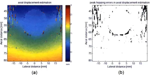
In fact, median filtering is required only in the region where those artifacts occur, but not in the whole field of view. Figure 3-10 shows simulated axial displacement estimation results and the locations where peak-hopping errors occur (see Chapter 4 for the simulation framework.) Figure 3-11 shows the spatial distribution of the correlation coefficients computed from axial displacement estimation and the locations where the coefficients are lower than the threshold value 0.5. The high correlation between the occurrence of peak-hopping errors and low correlation coefficients is demonstrated
through the comparison of Figure 3-10 (b) and Figure 3-11 (b).
Based on this observation, a filtering scheme with non-uniform spatial resolution is proposed to smooth the low-quality estimation results while reserving the spatial resolution in the region of high-quality estimation. The value of correlation coefficient is used as an indicator of the quality of displacement estimation. At the locations of
low-quality estimation, 9 x 9 median filtering is applied. Then the whole field of view
is smoothed by another 5 x 5 median filtering.
axial displacemeri esimation
70 2 2 1' 80 -15 -10 -5 0 5 10 15 m
Lateral distance Immi
(a)
Figure 3-10 (a) simulated axial displacement indicate the occurrence of peak-hopping errors
peak-hopping errors in axial displacement estimation
70
75
80
-15 -10 -5 0 5 10 15
Lateral distance Imm
(b)
estimation results; (b) the black dots in the estimation results
correlation values in estimation
Lateral distance (mim]
(a)
low correlation values in estimation
-15 -10 -5 0 5 10 15 Lateral distance Imm
(b)
Figure 3-11 (a) computed correlation coefficients in axial displacement estimation; (b) the black dots indicate the locations where the correlation coefficients are lower than
3.3 Polynomial Curve Fitting
After the trajectory field is established from the acquired sequence of ultrasound images, the image under a specified contact force can be estimated from the field. If the specified force lies within the range of the acquired forces, linear interpolation is performed on the trajectories between the two acquired forces that enclose the specified force. On the other hand, if the specified force is beyond the acquired force range, extrapolation is performed on the trajectories.
Here the ordinary least-square curve fitting is used to perform extrapolation. Polynomial curves with varying orders are examined, which can be expressed by Equation (3.6a) and (3.6b)
N
Xij(f) = ai,j,k -fk (3.6a)
k=0 N
Yi,(f) = f#i,,k fk, (3.6b) k=O
where xtj and yij are the lateral and axial coordinates, respectively, of the pixel located
at the position (i,
j)
of the reference image. a andplare
the parameter sets that are to bedetermined in the curve fitting procedure.fdenotes the contact force and N denotes the order of the polynomial curves.
It is widely reported that, when compressed under a wide range of forces, biological tissue exhibits significant nonlinear mechanical behaviors. [25] Therefore, to characterize the pixel trajectories, polynomial orders up to the number of acquired frames minus one are tested. The results are presented and discussed in Section 4.3.
3.4 Summary
This chapter provided a detailed introduction to the trajectory-based deformation estimation and correction method, which consists of 2D displacement estimation on the acquired ultrasound images and polynomial curve fitting on the established trajectory
field. The displacement estimation method is based on a template matching scheme, in which the search is performed using a coarse-to-fine approach. Correlation coefficients are used as the similarity measure, and the correlation filtering method is incorporated to improve correlation estimation. Two-dimensional curve fitting is used to provide subsample estimation accuracy. Finally, a smoothing scheme with non-uniform spatial resolution is proposed to filter out noise while preserving high spatial resolution in regions of high quality estimation.
Chapter 4
Ultrasound Simulation Using
Finite-Element Methods
In this chapter, compression of biological tissue and acquisition of the corresponding ultrasound images are simulated by using Finite-Element Methods (FEM) and the ultrasound simulation software Field II [26],[27]. The setup of simulation is described in Section 4.1.
Through the use of the simulated images and the FEM ground truth, performances of displacement estimation, extrapolation by polynomial curve fitting, and deformation correction are examined. These results are presented and discussed in Section 4.2-4.4, respectively.
4.1 Simulation Setup
The simulation framework consists of breast tissue modeling both in FEM and Field II.
A numerical tissue phantom was built in FEM to characterize the mechanical behaviors
of breast tissue under probe contact. A corresponding phantom was built in Field II for simulating ultrasound images of the numerical phantom in FEM under varying deformation states. Note that although simulation in this chapter is performed assuming that breast tissue is under investigation, the framework described is applicable to any kind of soft tissue.
4.1.1 FEM
A 100 mm x 60 mm numerical phantom that models breast tissue was built in
commercial FEM software (Abaqus 6.8, HKS, Rhode Island). Inside the phantom, a
circular region with a radius of 7.5 mm was delineated to mimic pathological tissue,
and the center was placed 22.5 mm below the top surface of the phantom. The whole phantom was then meshed into 3724 plane strain quadrilateral elements with 3825 nodes, as shown in Figure 4-1. FEM simulation was set to be two-dimensional, that is, in the axial and lateral directions. Deformation of the numerical phantom in the elevational direction is ignored, which is consistent with the assumption in the displacement estimation algorithm
measure the reaction
force at the point a fixed rigid Indenter that
mimics an ultrasound probe
pathological tissue
60rnm
i
normal'tissueproperties
~propertis
100mm
a rigid plane pushing upward
Figure 4-1 The setup in FEM
The mechanical behaviors of the phantom undergoing finite strains were characterized by hyperelastic models, as significant nonlinear behaviors of compression on biological tissue are widely found.[25] In addition, the simulated tissue was assumed to be isotropic and incompressible. Out of several hyperelastic models, such as the Neo-Hookean, Mooney-Rivlin, Yeoh, Arruda-Boyce, and Ogden models, the second-order polynomial model was selected as it has been suggested as a good fit of the mechanical behaviors of compressed breast tissue. [28] The model is described
by the strain energy function in Equation 4.1.
2 2
U = Cij(I1 - 3)i (12 - 3)j +{ (=ei - 1)2i, (4.1)
i+j=1 =1
where Uis the strain energy per unit volume,
h
and 12 are the first and second deviatoricstrain invariant, respectively, and
J,1
is the elastic volume strain. C's are the materialparameters with the units of force per unit area, and
Ds
are compressibilitycoefficients that are set to zero for incompressible materials.
In the numerical phantom, normal breast tissue was characterized by the 40
hyperelastic properties of adipose, and pathological tissue by those of low grade invasive ductal carcinoma (IDC), as IDC is the most commonly observed breast cancer. The hyperelastic parameters of those tissue types can be estimated from ex-vivo
experiments and are reported in [25] and [28]. These parameters are summarized in
Table 4-1.
Table 4-1 The hyperelastic parameters of normal and pathological breast tissue in FEM
C1 COI Cu1 C20 C02
Adipose 3.1 3.0 22.5 38.0 47.2
Low grade lDC 30.8 30.8 94.2 94.2 1390
unit: 104N mm2
A rigid indenter mimicking an ultrasound probe (vermon LA 5.0/128-522) was
modeled and used to compress the phantom against the rigid plane at the bottom. Compression was performed in a quasi-static manner for describing very slow motion and ignoring inertial effects. It should be noted that, in ultrasound scanning, the subject is scanned with respect to the probe. Therefore, features in the phantom would appear to be moving upward in the image when being compressed, while they would actually move downward physically. In order to describe tissue deformation measured in the coordinate system of the probe, in the simulated compression, the probe was fixed and the rigid plane was set to move upward.
4.1.2 Field II
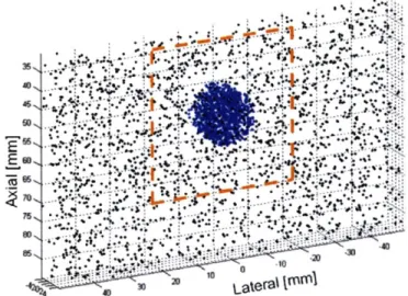
To simulate the ultrasound images of the numerical phantom in FEM, a corresponding
phantom was modeled in the ultrasound simulation software Field II. 2x 10⁵ scatterers
were randomly distributed in a 100 mm x 60 mm x 10 mm cube to simulate the
behavior of tissue reflecting ultrasound waves. The top surface of the phantom was set to be 30mm below the probe. A sampled set of the scatterers is shown in Figure 4-2. The circular region marked in blue corresponds to the simulated pathological tissue in FEM and was set to have a higher average of acoustic impedance in Field II. The rectangular region bounded by dashed lines indicates the field of view in the simulated ultrasound scan. The ultrasound images of the numerical phantom in varying
deformation states were simulated by relocating the scatterers according to the results of nodal displacement measurement in FEM deformation analysis.
Figure 4-2 A sampled set of the scatterers in ultrasound simulation
Here in the simulation, a linear probe array was modeled, with a center frequency
of 5 MHz and a sampling rate of 60 MHz. The transmit focus was set to be 55 mm in
depth. The pitch of the probe array was 0.3 mm, and 64 elements were used for every scan line. An image was composed of 128 scan lines, with a spatial spacing of 0.3 mm in the lateral direction.
4.2 Displacement Estimation
The displacement estimation method described in Section 3.2 is evaluated in this section. Specifically, the performance improvement from using the coarse-to-fine search scheme and incorporating correlation filtering are examined through the use of the simulated data. Subsequently, the influence of parameter selection on the performance of displacement estimation is examined.
4.2.1 Single-Level and Coarse-to-Fine Search
Section 3.2 describes a 2D displacement estimation method that incorporates
coarse-to-fine search, correlation filtering, and subsample estimation. This particular search scheme is termed "filtered coarse-to-fine" in this section. It is compared with the single-envelope, single-RF, and coarse-to-fine search scheme. Single-envelope and single-RF refer to the single-level correlation-based search scheme that uses envelopes and RF data, respectively, of ultrasound waves for template matching. Coarse-to-fine is the same as the filtered coarse-to-fine scheme except that correlation filtering is not
incorporated.
The parameters in each implementation of the search schemes are summarized in Table 4-2. Under the simulation setup, the axial search length of 3 mm corresponds to a maximum detectable strain of 5%. For single-envelope and single-RF, the search is performed on the original spatial resolution as in RF data acquisition, with a sample spacing of around 12.8 tm. For the coarse-to-fine scheme, 4-to-i decimated samples with a spacing of around 50 pm are used in coarse scale, and the original resolution is used for fine scale. Note that given these parameter settings, the computational cost for the coarse-to-fine search schemes is less than 10% of that for single-level search.
Table 4-2 Parameters for the search schemes
search scheme parameter # samples value (mm)
single-envelope kernel length 311 4
axial search length 234 3
single-RF kernel length 311 4
axial search length 234 3
coarse-to-fine kernel length (coarse) 77 4
axial search length (coarse) 58 3
kernel length (fine) 155 2
axial search length (fine) 7 0.09
correlation filter length 29 1.5
In addition, to examine the influence of noise on the performance of each search scheme, three major sources of waveform decorrelation are modeled. They are:
1. Applied strain: when the strain becomes larger, the intra-kernel deformation effect
between pre- and post-compression waveforms becomes more prominent, thus making it less appropriate to approximate displacement estimation as a time delay
problem. The examined strain levels are from 1% to 5%, with a spacing of 1%. 2. Elevational offset: the spatial shift of the probe in the elevational direction
introduces decorrelation between the pre- and post-compression waveforms. The examined elevational offsets are from 0 to 0.4 mm, with a spacing of 0.1 mm.
3. Signal-to-noise ratio (SNR): the quality of signal could also be influenced by other
factors, such as the thermal noise inherent in the hardware, the reverberation of ultrasound waves, patient motion artifacts, and so on. They are collectively modeled as additive white Gaussian noise (AWGN) in this analysis. The examined SNR levels are from 10 dB to 50 dB, with a spacing of 10 dB.
In the above framework, the estimation accuracy and robustness of each search scheme are compared. The accuracy is quantified by the mean absolute errors (MAE) between the displacement estimation results and the FEM ground truth. The robustness is characterized by the occurrence rates of the axial peak-hopping error, which is defined as an error larger than half of the carrier wavelength. At each noise setup in the following analysis, each search scheme was evaluated 25 times. For each independent trial, there was a different realization of the ultrasound simulation (i.e. different random locations of Field II scatterers) and random AWGN. The curves indicate the mean values of the results, and the error bars indicate one standard deviation.
Figure 4-3 shows the change in MAE and peak-hopping errors with the applied strain level in axial displacement estimation. The elevational offset is set to be zero, and SNR is set to be 30 dB. As expected, when the strain becomes larger, estimation is more error-prone for all the examined schemes. Nevertheless, it is obvious that the coarse-to-fine search scheme is more accurate and robust than single-level search in the presence of a high strain level, and coarse-scale correlation filtering brings noticeable improvement in displacement estimation. Similar observations can be made from analysis of elevational offsets (Figure 4-4), where the strain level is set to be 2% and