Degree Correlations and Motifs in Technological Networks

E

Ennggiinneeeerriinngg SSyysstteem

mss D

Diivviissiioonn

Working Paper Series

ESD-WP-2005-10

D

EGREE

C

ORRELATIONS AND

M

OTIFS IN

T

ECHNOLOGICAL

N

ETWORKS

Daniel E. Whitney

MIT Engineering Systems Division dwhitney@mit.edu

Degree Correlations and Motifs in Technological Networks

Daniel E. Whitney

MIT Engineering Systems Division Room E40-243

77 Massachusetts Ave Cambridge MA 02139 e-mail: dwhitney@mit.edu

ABSTRACT

Recent network research has sought to characterize complex systems with a number of statistical metrics, such as power law exponent (if any), clustering coefficient, community behavior, and degree correlation. A larger goal of such research is to obtain insight into the systems’ functions by means of these and similar analyses. In this paper we examine network models of mechanical assemblies. Such systems are well understood

functionally. We show that they have both rich and varied community structure as well as negative degree correlations (disassortative mixing), and show that this can be

explained by additional powerful constraints that arise from identifiable first principles. In addition, we note that their main “motif” is closed loops (as it is for electric and

electronic circuits), a pattern that conventional network analysis does not detect but which is used by software designed to aid in the design of such systems. The implication is that functional understanding of complex systems requires considerable domain knowledge beyond what typical network analysis tools employ.

I. Motivation

Recent network research has sought to characterize complex systems with a number of statistical metrics, such as power law exponent (if any), clustering coefficient, community behavior, and degree correlation. Use of such metrics represents a choice of level of abstraction, a balance of generality and detailed accuracy. It has been noted that “social networks” consistently display clustering coefficients that are higher than those of random or generalized random networks, that they have small world properties such as short path lengths, and that they have positive degree correlations (assortative mixing).

“Technological” or “non-social” networks display many of these characteristics except that they generally have negative degree correlations (disassortative mixing). [Newman 2003i] It has been shown that positive degree correlation and high clustering in social networks can be explained by the fact that they have no more than one edge between any pair of nodes (typical) and they display community structure with some variety in

community size. [Newman and Parkii] On this basis it is said that “social” networks are the exception in having positive degree correlation, and that others must of necessity display low clustering and negative degree correlations because they do not display community structure.

In this paper we examine a kind of technological network about which the author has considerable domain knowledge, namely mechanical assemblies. We have several objectives:

o To see whether these networks conform to other technological networks in their typical statistical properties, compared to those in [i]

o To see what particular properties they have because they are mechanical assemblies

o To explain why they display negative degree correlation even though they have rich community structure and high clustering coefficients

o To see what can be learned about their underlying function by examining them using the network analysis methods used by network researchers and to indicate what other tools are important in understanding them

II. Literature

Recent network analysis research has evolved from studying scale-free behavior [Albert and Barabásiiii] to a search for understanding the functional behavior of systems. Newman [1] states that the search for functional understanding is in its infancy and is the ultimate goal of the research. Various authors have studied software [Myersiv], the Internet [Li et alv], biological systems [Milo et alvi], [Ravasz et alvii], and electronic circuits [Ferrer I Cancho et alviii], among others. Each of these authors sought to find, with varying degrees of success, relationships between network statistics or structure, usually in the form of clusters (sometimes called modules) or internal patterns, and function. Deeper study has indicated that complex networks can be classified by domain, such as social,

informational, biological, and technological, and their statistical properties compared [i Table II]. Both [vi] and [Itzkovitz et alix] found repeating internal structures in various systems and had some success in linking them to functions. Others have sought to find clusters (highly linked sets of nodes that do not necessarily form repeating patterns), among them [Newman 2004x], and formulated a method for finding them [Girvan and

networks formed layers of similar structures but a different structural pattern in each layer, which they called “scale rich” and “self-dissimilar.” [v] showed that the structure of the Internet depends at least in part on technological constraints imposed by the design of the routers. [Whitney 1996xii] argued that technological systems that process large amounts of power are less likely to display strong modular structure than those which process information at essentially negligible power levels. [ii] offered an explanation for positive Pearson degree correlation in social networks and negative degree correlation for other types. Each of these papers indicates that some domain knowledge is necessary in order to understand the relationships between network structure and statistics on the one hand and function on the other.

This paper focuses on mechanical assemblies and network methods for understanding them. [Bourjaultxiii] introduced the “liaison” graph model of assemblies in which a part is represented by a node and a joint between parts by an edge and used network and circuit theory to find all possible assembly sequences. [Björkexiv] is one of many authors who use network methods to analyze tolerances and predict propagation of part size and shape variation in assemblies. Assemblies are equivalent to kinematic mechanisms, whose motion and constraint properties have been analyzed by network methods for decades [Phillipsxv], [Whiteheadxvi], [Blandingxvii], [Konkar and Cutkoskyxviii], [Shukla and Whitneyxix], [Whitney2004xx].

The paper is organized as follows: Section 0 describes assemblies generically and illustrates how their clustering and community structure arise. Section 0 provides basic statistics on a number of assemblies as an addition to Table 2 in [i]. Section 0 derives a powerful internal constraint on assemblies from first principles. Section 0 shows that this

constraint and important engineering design principles can explain why assemblies can simultaneously display rich community structure and negative degree correlation. Section 0 shows that the main functional motifs of assemblies and other technological systems are closed loops, which typical network analyses do not look for, and that clusters and

communities do not account for function as well as loops do. Section 0 concludes the paper with discussion and conclusions.

III. Some Properties of Assemblies

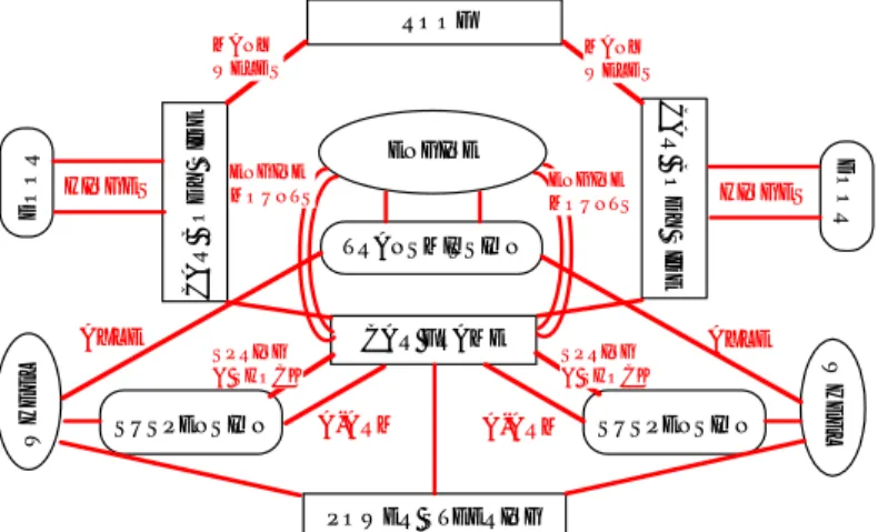
Mechanical assemblies are definitely technological networks. Compared to the Internet, mechanical assembly networks are small, but they can be comparable in size to food webs and other recently studied networks, often having in the low to mid hundreds of nodes and edges.1 Assemblies are typically designed to have a hierarchical structure, with subunits called subassemblies, which can be nested to a few levels (perhaps three to five, sometimes more). A hierarchical decomposition of an automobile might have top level assemblies {body, chassis, power train, interior} with respective main subassemblies {roof, car body side, car frame, doors, hood, trunk lid}, {springs, shock absorbers, steering gear}, {engine, transmission, drive axles, brakes}, and {seats, dashboard, steering wheel, shifter console, interior trim}, and so on. Figure 1 shows some of these subassemblies and the main liaisons between them. Similarly, aircraft have top-level assemblies {fuselage, engines, landing gear, control systems, interior} with corresponding subsystems.2

1 _{Assemblies are always modeled as undirected networks.} 2

ENGINE TRANSMISSION CAR FRAME CAR BO DY SIDE CAR BO DY SIDE SUSPENSION SUSPENSION WHEEL WHEEL D OOR D OOR ROOF HINGES HINGES AXLE AXLE A-ARM A-ARM SPRING & SHOCK SPRING & SHOCK ENGINE MOUNTS MANY WELDS MANY WELDS ENGINE MOUNTS POWER STEERING

Figure 1 Notional Network Diagram of a Car. A car is made of a large number of complex subassemblies containing from dozens to hundreds of parts. They join to each other at relatively few places. Except for the liaison called “many welds,” the liaisons in the figure are shown in their correct cardinality. Thus, the door joins the body side via the two hinges shown. The engine joins the transmission via the crankshaft and a bolted joint. Not shown are other complex subassemblies with the same properties, such as seats and instrument panel. Within each complex

subassembly are other complex sub-subassemblies that in turn join to their parents via a relatively few liaisons.

The main subassemblies often have more parts than their parent assemblies, and there is typically considerable diversity in size, shape, technological content, operating principles, and so on, giving rise to self-dissimilarity, clustering, “community structure,” and

heterogeneity. These properties are strongly driven by engineering, performance,

manufacturing, field repair, and supply chain forces which are too numerous and complex to discuss here but are the focus of an enormous literature.

When assemblies are modeled as networks where parts are nodes and an edge or liaison represents the fact that two parts assemble to each other, the resulting networks have a

ratio of edges to nodes that almost never exceeds 2.1 and averages around 1.6. The reason for this is a pervasive internal constraint that we show is also the root of their negative degree correlation. Data on assembly networks is discussed next.

IV. Statistical Properties of Assemblies

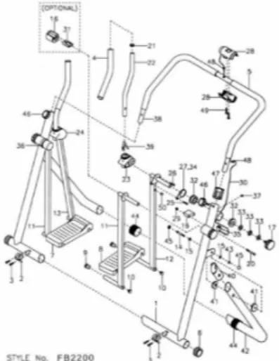
In this Section, we give in Table 1 the usual statistics about some assembly networks and compare them to Table 2 in [i]. The subject assemblies are, in increasing order of number of nodes, a rifle, an exercise walker, a model airplane engine, a bicycle, and a V-8

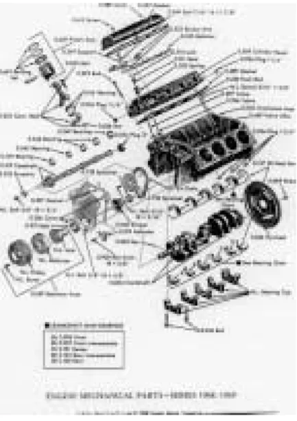
automobile engine. Three of these items are depicted in Figure 2, Figure 3, and Figure 4.

Figure 2 Exercise Walker Exploded View

Figure 4 V-8 Engine Exploded View. This engine is similar to but not exactly the same as the one analyzed in Table 1 and later in the paper.

Item n (number of nodes) m (number of arcs or edges) Ratio of m to n and [mean degree] Clustering

coefficient* Average path

length Random path length ln(n) /ln(<k>) Random clustering coeff <k>/ n Generalized random clustering coeff <k> n <k2 > − <k> <k>2       2 Degree correlation (Pearson) 1885 Winchester Single Shot Rifle 35 54 1.54 [3.09] 0.309 3.121 3.16 0.088 0.099 -0.177 Hyper 21 Model Airplane Engine 45 65 1.444 [2.889] 0.388 3.579 3.588 0.064 0.10 -0.235 Walker ** Figure 2 75 124 1.6 [3.2] 0.623 2.812 3.17 0.08 0.179 -0.213 Bicycle*** Figure 3 235 364 1.59 [3.175] 0.415 4.051 4.22 0.024 0.082 -0.202 V8 Engine**** Figure 4 462 684 1.512 [3.024] 0.225 4.345 4.964 0.0124 0.192 -0.2695

Table 1. Properties of Some Mechanical Assembly Networks. *Clustering Coefficient calculated ignoring nodes whose nodal

clustering coefficient = 0. **The walker assembly is symmetric and only half of it was analyzed. The version analyzed has 40

nodes and 64 edges. ***The bicycle was analyzed using only 10 identical spoke sets on each wheel, whereas the front has 32

and the rear has 40. Thus the version analyzed has 131 nodes and 208 edges. ***The engine network contains only 8 of the

omitted. Clustering coefficient and path length calculated using UCINET v 6.9 [Borgatti et alxxi]. Pearson correlation

As can be seen by comparing to Table 2 in [i], these networks conform to the

expectations and existing data for “technological” networks. They also display typical small world properties (larger clustering coefficient than random or generalized random

networks with the same n and m, and short path length). Their path lengths are

indistinguishable from those of random graphs with the same number of nodes and edges. While they are generally too small to be examined for power law behavior, their highest

degree nodes obey kmax > n, providing sufficient range in k to permit comparison with

the conditions for positive degree correlation used by [ii].

V. Mean Degree of Assemblies

It was stated above that the limit on mean degree in assemblies arises from a powerful internal constraint. This constraint is discussed here, first empirically and then

theoretically.

Figure 5 shows the distribution of average network connectivities (number of edges or liaisons divided by number of nodes or parts; equivalently half the average nodal degree

<k>) for several commercial products such as mechanical toys, cordless screwdrivers,

staple guns, and car and truck transmissions. Also shown are the theoretical maximum and minimum values for this metric for each product. It is notable that, with one exception discussed below, the products shown do not have nearly the connectivity that they theoretically could, based on how many nodes they have, if they were either random graphs or Albert-Barabási [iii] growth-preferential attachment scale free networks. In fact, the metric rarely takes on a value above 2. The reason for this is based on fundamentals of kinematics.

Liaisons per Part 0 2 4 6 8 10 12 14 16 18 Ballpo int Pe n Rear Axl e Juic er Thro ttleb ody _Seeker Elec tric Iron B&D Co rdle ss Scre wdr iver 6 Sp eed Tra nsmi ssion Tran saxl e Sear s Cord less Scre wdri ver Car Body Side Cui sina rt Mi niP rep Che aper St aple r Elect ric D rill Car Inst rum ent Pa nel Rugg ed S tapler Chin ese Puzzl e Liaisons/Part Min=(n-1)/n Max=(n-1)/2

Liaisons per Part

Figure 5 Network Connectivity Metric for Several Assemblies. [xx] The products in this chart have n = 10 to 30 parts or more, and the potential range of network

connectivities is large: min : (n−1) / n; max : (n−1) /2. But the maximum connectivity potential is not realized by any product surveyed with the exception of the “Chinese puzzle.” Instead, actual connnectivities hover near the minimum, and the maximum does not exceed about 2.1.

Figure 6 shows data from [Greerxxii] on the network connectivity of a number of

household products over several redesign generations. Each generation represents

application of Design for Assembly principles [Boothroyd, Dewhurst, and Knightxxiii],

primarily simplification and part-count reduction, as well as aggressive cost reduction implemented by materials and process substitutions. Metals were replaced by polymers, discrete fasteners were replaced by flex hinges or adhesives, metal forming was replaced by injection molding, for example. While Greer [xxii] was interested in the number of distinct parts needed to implement specific functions in these products (which falls steadily with each evolutionary stage), he also gathered information on the number of

parts and interfaces. Not only is the ratio of connections to parts similar to our data in Figure 5, but remarkably it is roughly constant over the generations for each product. Thus Greer’s [xxii] data are consistent with our own and demonstrate that this property extends across several design methodologies, materials choices, and manufacturing methods.

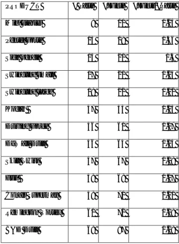
Table 2 shows data on the network connectivity of 14 products gathered by [Van Wie et al. xxiv] These are household products similar to those surveyed by [xxii] and have a similar average nodal degree. The range of connectivity in these datasets is narrower than that in Figure 5 but is consistent overall.

PRODUCT # Parts #Joints #Joints/#Parts

Mini stapler 8 10 1.25 Pentel Forte 13 19 1.46 Side pencil 15 21 1.4 Swingline small 17 21 1.24 Swingline large 18 22 1.22 Kodak 47 53 1.13 Driving Force 56 60 1.07 DeWalt Drill 56 64 1.14 Skill Twist 57 67 1.18 Fuji 58 68 1.17 Conair Supermax 58 70 1.21 Remington Vortex 61 72 1.18

Conair Quiettone 69 84 1.22

Average _1.225

Table 2 Network Connectivity Data for 14 Products Surveyed by Van Wie et al. [xxiv] 0 0.5 1 1.5 2 2.5 Orig inal Evo lutio n #1 Evo lutio n #2 Evol utio n # 3 Evol utio n # 4 Number of Evolutions Li nk Co nn e c ti v it y (I n t. I n te rf ac es / # C o mp o n e n ts ) BICYCLE 3-Bar BICYCLE 4-Bar ICE CREAM SCOOP TOOL CASE PENS STAPLE REMOVER CLOTHES HANGER BICYCLE BRAKE BOTTLE CAP CD CASE CLOTHES PIN FORCEPS COMPLIARS KITCHEN CLIP TOOL HOLDER WIRE STRIPPER

Figure 6 Data from [xxii] Showing Network Connectivity for Several Generations of the Same Product. Each later generation exhibits fewer parts and fewer parts per implemented function but roughly the same network connectivity. The average network connectivity for this data set is 1.24.

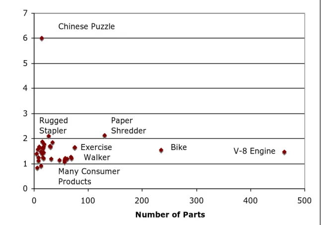
Figure 7 shows that the network connectivity of parts in assemblies having from 6 to 245 parts does not increase with the number of parts. In both real world scale free and

random networks, it is predicted that connectivity should grow with the number of nodes. [iii] For the data available, mechanical assemblies do not behave this way. Assemblies with more than 100 or 200 parts are rare, for reasons cited above. Figure 7 also shows visually the fact that, except for the Chinese Puzzle, network connectivities for these

0 1 2 3 4 5 6 7 0 100 200 300 400 500 Number of Parts Chinese Puzzle Paper Shredder V-8 Engine Many Consumer Products Rugged Stapler Exercise Walker Bike

Figure 7 Liaisons Per Part vs Number of Parts for 35 Mechanical Products. There is no correlation between the network connectivity of these assemblies and the number of parts in them. The Chinese Puzzle is an outlier for reasons discussed in the text. The average connectivity for this dataset is 1.55, close to the value for the V-8 Engine (1.51). Data in this figure are a combination of those gathered by the author and those in [Van Wie, et al xxiv].

Figure 5, Figure 6, and Figure 7 show that typical assemblies do not have anywhere near

the connectivity that they might.3 To see a physical reason why, we begin by making the

analogy between mechanical assemblies and kinematic mechanisms. All mechanisms are

assemblies. While not all assemblies move in the sense that typical mechanisms do, assemblies nevertheless obey the same fundamental principles of statics. Among the issues of concern in kinematics is the state of constraint of the assembly: is it under-constrained and thus capable of movement; is it “exactly” under-constrained, having just enough links to prevent motion; or is it over-constrained, having more than enough links to prevent motion? The last case is considered undesirable [xvii], [xvi] because it could result in locked-in stress in the assembly, leading to assembly difficulties or field failure. The implication is that constraint plays the role of a limit or cost related to adding arcs to

a node, as suggested by [Amaral, et alxxv] for other kinds of networks.

The Grübler criterion [xv] is typically used to determine the numerical value of the number of degrees of freedom M in a planar mechanism:

Equation 1 M =3 n

(

)

∑

f_i =degrees of freedom of joint i

If M >0, the mechanism has M under-constrained degrees of freedom. If M <0, the

mechanism has M more links than necessary to prevent motion and is over-constrained.

If M =0, the mechanism is exactly constrained. If we define

α

connectivity) and define the average number of degrees of freedom allowed per joint as

β

α

β

αβ

∑

(

α

)

αβ

(

)

(

)

Note that unless

β

α

Furthermore, larger

α

β

the mechanism is to be exactly constrained, then M =0 and Equation 2 can be solved for

α

α

(

β

)

β

This expression is based on assuming that the mechanism is planar. If it is spatial, like all those in Table 1, then “3” is replaced by “6” and Equation 1 is called the Kutzbach

criterion, but everything else stays the same. Table 3 evaluates Equation 3 for both planar and spatial mechanisms.

β

α

α

0 1 1

1 1.5 1.2

Table 3. Relationship Between Number of Liaisons Per Part and Number of Joint Freedoms for Exactly Constrained Mechanisms (M=0).

Table 3 shows that

α

over-constrained. If a planar mechanism has several two degree-of-freedom joints (pin-slot, for example) then a relatively large number of liaisons per part can be tolerated. But this is rare in typical assemblies. Otherwise, the numbers in this table confirm the data in Figure 5, Figure 6, and Figure 7. Most assemblies are exactly constrained or have one

operating degree of freedom. Thus

β

β

α

with our data. The products in Figure 6 and Table 2 are simpler in most cases than those in Figure 5 so it is not surprising that the former have smaller average network

connectivity than the latter.

The Chinese Puzzle is an outlier because it is highly over-constrained according to the Kutzbach criterion. It is possible to assemble only because its joints are deliberately made loose. Nonetheless, the overabundance of constraints is the reason why it has only one assembly sequence, that is, why it is a puzzle.

VI. Degree Correlation of Assemblies

The Pearson degree correlations ( r) of a number of networks have been calculated and it

has been noted that “social” networks tend to have positive values of r while

“technological” and other “non-social” networks tend to have negative values. [i] While, as Newman says, there is unlikely to be a single explanation for this for all types of networks, [ii] have shown that networks with rich community structure and a maximum

The mechanical assemblies in Table 1 all have negative values of r. Here we show that they also have rich community structure as calculated by the Girvan-Newman algorithm (as implemented in NETDRAW [xxi]). We show the network diagrams of the walker, the bicycle, and the V-8 engine respectively in Figure 8, Figure 10, and Figure 10. The communities identified make good sense. They are relatively numerous and have a dispersion of sizes. Thus the networks fit the requirements in Newman and Park as being

candidates for positive r, but display firmly negative r. On this basis we conclude that

the Newman-Park criterion may explain social networks but that these technological networks have other properties not accounted for by the Newman-Park model.

In spite of making good sense, the identified communities do not tell a lot about how the products work. Instead, we need to understand the assemblies functionally more deeply.

Figure 8. Network Diagram of the Walker, Showing Community Structure. The most highly connected and functionally important nodes in each community are named. (Color Online)

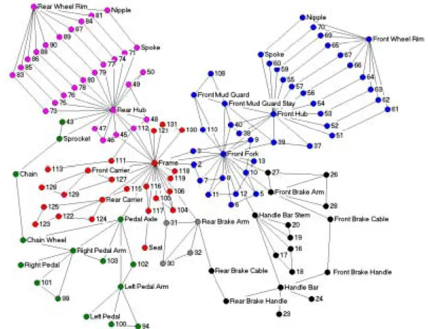
Figure 9. Network Diagram of a Bicycle. The most highly connected and

functionally important nodes in each community are named. Only 10 of 32 front (40 rear) spokes and nipples are shown and used in the analysis in Table 1. (Color Online) Head Block Crankshaft Camshaft 2 Crank Cvr Camshaft 1 Wires Intake Manifold Oilincvr Acc Belt Chain Tens Crank Chain 13 Piston 1 15 16 17 18 19 20 21 22 Valve 1 24 25 26 27 28 29 30 31 32 Rod 1 34 35 36 37 38 39 40 L M Brg 1 42 43 44 45 U M Brg 1 47 48 49 50 51 52 Crank Gear 54 55 Foll 1 57 58 59 60 61 62 63 64 Rod Cvr 1 66 67 68 69 70 71 72 Wrist P 74 75 76 77 78 79 80 81 Top Ring 1 83 84 85 86 87 88 89 90 91 92 93 94 95 96 97 98 99 100 101 102 103 104 105 106 107 108109 110 111 112 113 114 115 116 Alternator 118 119 Cam Sprocket 2 121 122 123 124 125 126 127 Acc Pulley 129 Cam 1 131 132 Roller 1 134 135 136 137 138 139 140 Head Gask 142 143 144 Cam Sprocket 1 146 147 148 149 150 151 152 153 154 155 156 157 158 159 160 ₁₆₁ 162 163 164 Plug 166 167 168 169170 171 172 Intake Gask 174 175 176 177 178 179 180 181 182 183 184 185 186 187 188 189 ₁₉₁₁₉₀ 192 193 194 195 196 197 198 199 200 201 202 203 204 205 206 207 208 209 210 211 212 213 214 215 216 217 218 219 220 221₂₂₂ 223 224 225 226 227 228 229 230 231 232 233 234 235 236 237 238 239 240 241 242 243 244 245 246

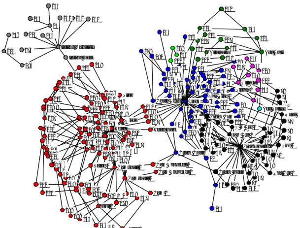
Figure 10. Network Diagram of V-8 Engine Showing Community Structure. The most highly connected and functionally important nodes in each community are named. Other nodes are named to help readers understand and navigate the network, and for use in Figure 11. (Color Online)

Why do these (and, most likely, many other) mechanical assemblies have negative r?

First, from a numerical standpoint, negative r goes with the tendency for highly

and vice versa. From a functional point of view, highly connected nodes in a mechanical assembly typically play either high load-carrying or load-distributing roles, or provide common alignment foundations for multiple parts, or both. The frames, pivot pins, and pedal arms of the walker, the frame and front fork of the bicycle, and the cylinder block, cylinder head, and crankshaft of the engine perform important load-carrying functions in their respective assemblies. In a clock or watch, two parallel plates align a number of gear wheels that in turn mate to each other in an open chain. The two plates, high degree nodes, mate only to the low degree gear wheels, plus to posts that mutually align the plates. The more gear wheels there are, the more negative the degree correlation will be, in spite of the fact that all the low degree nodes mate typically to two others.

It is worth noting that almost without exception these highly connected nodes do not connect directly to each other. In high power assemblies like engines, there are always interface parts, such as bearings, shims, seals, and gaskets, between these parts to provide load-sharing, smoothing of surfaces, or other services. Such interface parts are necessary and not gratuitous.

In addition, because they are often big, so as to be able to withstand large loads, these parts have extensive surfaces and can act as foundations for other parts that would otherwise have no place to hang on. On the engine, such parts include pipes, hoses, wires, pumps and other accessories, and so on. Several of these must be located accurately on the block with respect to the crank but many do not.

Recalling the discussion of constraint above, it is noted that some of the highly connected nodes, most importantly the block and crankshaft, are over-constrained when considered together with the parts they mate to, such as camshafts and connecting rods. This is

unavoidable, and gives rise to the need for considerable precision in their manufacture and assembly. But if these already highly constrained and high-degree nodes mated directly to each other, the ensemble would be hopelessly over-constrained and essentially impossible to manufacture efficiently. However, the parts that merely “hang on” to the block do not impose additional constraint. Additionally, these “hanger-oners” usually do not carry large loads and tend therefore to be weakly connected, reinforcing the negative

value of r.

Finally, most assemblies have only a few high-k foundational, load bearing, or common

locating parts, and many other parts mate to them while mating with low probability to each other. Thus even if the high k parts mated to each other, the assortativity calculation

would be overwhelmed by many (high k – low k) pairs, again yielding negative values

for r.

Thus negative degree correlation in assemblies can be seen as a consequence of the need to avoid over-constraint. Yet these same assemblies display rich community structure, as described in Section 0. Thus the need to avoid over-constraint apparently overpowers the conditions favoring positive degree correlation in social networks. Similar internal constraints may act in other technological networks.

Social networks apparently do not have to support such powerful internal constraints or

costs of multiple connections, and thus can display positive r. Indeed, the edges in an

assembly, and most technological networks, are “always on” and have the same high strength. In social networks like co-authorships, authors need not communicate simultaneously with all their present and past co-authors. Actors need not deal in one

nodes can “exist” without affecting each other. Equivalently, many links can be very weak at times, whereas the links in an assembly or electric/electronic circuit are at full strength all the time.

VII. Functional Motifs of Assemblies

The heritage of social network analysis has bequeathed to us a number of analysis tools that seek in networks the kinds of features that are important for social science, such as path length, clustering coefficient, community structure, and power laws. However, in many technological networks, the motifs that generate function are closed loops. This is certainly true for both mechanical assemblies and electric/electronic circuits, whether they operate at high or low power. Methods for designing and analyzing mechanisms and

circuits via loop methods have been in use for over a century.4 High k nodes are

certainly important for the reasons mentioned above, but the loads or mutual locations in question operate in support of higher-level functions that are implemented by loops. In the Walker, the loops cannot be seen until a person is added. This person exerts vertical loads on the pedals via gravity and horizontal back and forth loads on the handles and pedals while exercising. The horizontal load loops pass from the person’s arms and hands to the walker’s handles, then to the frame, then to the pedals, then into the person again via the feet and legs. The vertical load loops do much the same except that they contain an invisible gravity segment that exits the person’s body, enters the earth, and

4

In electric circuits, one simply finds any spanning tree and systematically closes the open ends. If the

circuit is linear, the superposition principle applies, and the circuit’s behavior can be analyzed using any set

returns to the walker via the feet on the frame. Similar loop logic can be applied to the bicycle.

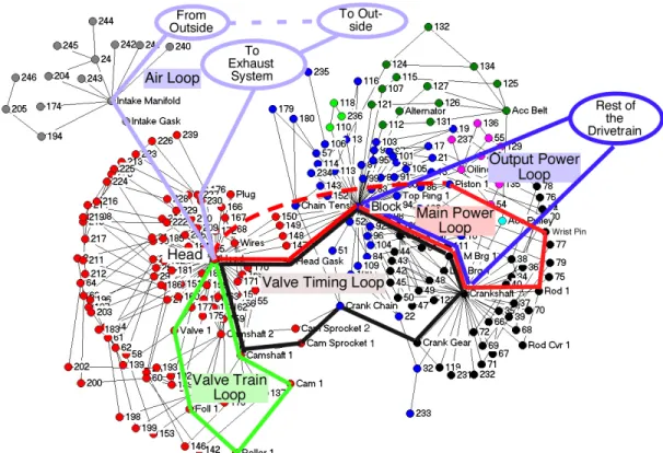
In the Winchester rifle, the mechanism has four states (empty, loaded, cocked, and fired). Transitions between these states open or close edges in the graph and consequently create or destroy different loops. Only one of these states was analyzed for inclusion in Table 1. The V-8 engine’s main loops are shown in Figure 11. Some loops are contained entirely within the engine while others (air, output power) close only when other parts of the car or its environment are included. Note that some of them stay within the identified communities while others extend beyond or link and coordinate different communities. These loops cannot be drawn by inspecting the graph but require domain knowledge. The clustering coefficient of a network is obtained by counting triangles, that is, by enumerating the shortest possible loops (length = 3). In general, the operative loops of an assembly are longer than three (typically 6 or 8) [xx] and thus do not contribute to the clustering coefficient. In fact, the conventionally defined clustering coefficient reveals nothing about the presence, number, or length of loops longer than three. Software for

finding motifs5 would be helpful here, but only some of the motifs thus found would be

functionally significant, and domain knowledge would be needed to identify them. Since positive degree correlation is related to more kinematic constraint while negative degree correlation is related to less kinematic constraint, the degree correlation

calculation can be thought of as a simplified cousin of the Grübler-Kutzbach criterion, because the former simply counts links and considers them of equal strength, whereas the

latter uses more information about both links and nodes and can draw a more nuanced conclusion. The most general method of characterizing mobility and constraint, which

removes a limitation in the [xix] network method, is that of Davies [Davies 1981xxvi]

[Davies 1983xxvii]. This method is based on identifying closed loops and comprises a

generalization to 6 dimensions of the familiar Kirchoff loop and node laws from electric circuit analysis. This fact reinforces the dominance of closed loops as necessary for understanding the behavior of these systems.

Most generally, an engine is an air pump. Its design is driven by the amount of desired power, which determines the required flow rate of air and fuel, which in turn determines the number and diameter of the cylinders and the piston stroke. These in turn drive the design of the main hubs plus essential cooling and lubrication systems (which are fluid flow loops). Various scaling laws drive larger engines to have more cylinders rather than one larger one. None of this is visible in the network diagram.

Figure 11. V-8 Engine with Five Main Functional Loops Indicated and Named. The main power loop shown is simplified, omitting parallel segments for the piston rings and an additional main bearing. It traces one of the 8 identical

crank-piston-cylinder-head loops in the engine. The valve train loop is also greatly simplified, omitting parallel segments that include springs and slack adjusters. It traces one of the 8 identical valve trains in the network as illustrated here. The edge in the main power loop shown in dashes represents burning gas pressure and is not strictly speaking a mechanical link between two parts. But it is functionally indispensable. (Color Online)

VIII. Conclusions and Discussion

At the beginning of this paper, we asked what can be learned about a complex system or family of systems by using widely applied network analysis methods. Here we have seen

One conclusion we can draw is that different kinds of systems have different operating motifs, and to understand a system is in some sense to know what those motifs are and how to find them. Tools for finding the independent loops in circuits and mechanisms have been used in commercial software since about 1970. The main task of designers of such systems consists of specifying and parameterizing the loops. Loops appear to be important in ecological, atmospheric, oceanographic, and climate systems as well. All of the assemblies analyzed here have a number of hubs. These are obviously

important parts but they do not perform functions by themselves. Instead, the identified functional loops seem to run from hub to hub. In systems where large amounts of power are involved, hubs often act as absorbers or distributors of that power or of static or dynamic mechanical loads. In other systems, the hubs can act as concentrators or

distributors of material flow or information flow. Generally, material, mechanical loads, and power/energy/information flow in closed loops in technological or energetic systems. All of the systems analyzed here display rich community structure with considerable variation in community size. All display negative degree correlation. The negative degree correlation can be readily explained via physical principles or engineering design reasoning. The communities identified by the Girvan-Newman algorithm make

functional sense in many cases but not others, and generally do not group items that form the functional loops.

Another, perhaps more tentative, conclusion is that functional knowledge is useful, perhaps necessary, in order to understand why a class of networks displays this or that characteristic, such as power law degree statistics, community structure, or positive (negative) degree correlation. The characteristics themselves, however, have limited

ability to provide insight into the “why” of a system’s network as compared to the “what.” A fundamental reason for this, illustrated by results quoted from [Greer], but well-known, is that there are many ways to implement the same function in a

technological system.

In some cases, such as judging the state of constraint of an assembly, the metrics alone can have important prescriptive value: over-constraint may be detrimental (though not always). A high-k node will be complex, costly to manufacture, and possibly at increased risk for failure (again not always, possibly unavoidable, and possibly the best way to design it after all).

For assemblies, the minimum domain knowledge required to learn much about the system is the connection graph plus information on the constraints applied on nodes by edges. Higher-level functional knowledge requires at a minimum knowing shape and mass properties of nodes. In electric circuits, one knows little without the connection graph and impedance information about the circuit elements themselves. With this information, almost everything about the circuit’s behavior can be explained.

Perhaps a useful way to characterize and group networks and systems is by the kind of information needed to determine their function at various levels of abstraction.

Acknowledgements

This paper benefited substantially from discussions with Professor Christopher Magee. The author would also like to thank Professors Dan Braha and Carliss Baldwin for stimulating discussions and Prof Mark Newman for sharing his software for calculating degree correlation. Many of the calculations in this paper were made using UCINET

i

M. E. J. Newman, SIAM Review 45, 167 (2003).

ii

M. E. J. Newman and J. Park, Physical Review E 68, 036122 (2003).

iii

R Albert and A-L Barabasi, Review of Modern Physics 24, 47 (2002).

iv

C. R. Myers, Physical Review E 68, 046116 (2003).

v

L. Li, D. Alderson, W. Willinger, and J. Doyle, SIGCOMM '04, Portland OR, (2004).

vi

R. Milo, S. Shen-Orr, S. Itzkovitz, N. Kashtan, D. Chklovskii, and U. Alon, Science

298, 824 (2002).

vii

E. Ravasz, A. L. Somera, D. A. Mongru, Z. N. Oltvai, and A.-L. Barabasi, Science

297, 1551 (2002).

viii

R. Ferrer i Cancho, C. Janssen, and R. Sole, Physical Review E 64, 046119 (2001).

ix

S. Itzkovitz, R. Levitt, N. Kashtan, R. Milo, M. Itzkovitz, and U. Alon, Physical

Review E 71, 016127 (2005).

x

M. E. J. Newman, European Physics Journal B 38, 321 (2004).

xi

M. Girvan and M. E. J. Newman, PNAS 99, 7821 (2002).

xii

D. Whitney, Research in Engineering Design 8, 125 (1996).

xiii

A. Bourjault, “Contribution á une Approche Méthodologique de l’Assemblage Automatisé: Elaboration Automatique des Séquences Opératoires,” Thesis to obtain Grade de Docteur des Sciences Physiques at l’Université de Franche-Comté, Nov, 1984

xiv

O. Björke, Computer-Aided Tolerancing (ASME Press, New York, 1989)

xv

J. Phillips, Freedom in Machinery (Cambridge University Press, Cambridge, 1984

xvi

T. N. Whitehead, The Design and Use of Instruments and Accurate Mechanism (Dover Press, 1954)

xvii

D. Blanding, Exact Constraint Design (ASME Press, New York, 2001)

xviii

R. Konkar and M. Cutkosky, ASME Journal of Mechanical Design 117, 589 (1995).

xix

G. Shukla and D. Whitney, IEEE Transactions on Automation Science and

Technology 2 (2), 184 (2005).

xx

D. Whitney, Mechanical Assemblies: Their Design, Manufacture, and Role in Product

Development (Oxford University Press, New York, 2004)

xxi

S. P. Borgatti, M. G. Everett, and L. C. Freeman, “Ucinet for Windows: Software for Social Network Analysis,” Harvard MA: Analytic Technologies, 2002.

xxii

Greer, James L., “Effort Flow Analysis: A Methodology for Directed Product Evolution Using Rigid Body and Compliant Mechanisms,” PhD Dissertation, University of Texas at Austin, 2002

xxiii

G. Boothroyd, P. Dewhurst, and W. Knight, Product Design for Manufacture and

Assembly (Marcel Dekker, New York, 1994).

xxiv

M. Van Wie, J. Greer, M. Campbell, R. Stone, and K. Wood, ASME DETC, Pittsburgh, DETC01/DTM-21689, (2001). ASME Press, New York, (2001).

xxv

L. Amaral, A. Scala, M. Barthelemy, and H. Stanley, PNAS 97, 11149 (2000).

xxvi

T. Davies, Mechanism and Machine Theory 16, 171 (1981).

xxvii