HAL Id: tel-00847076
https://tel.archives-ouvertes.fr/tel-00847076
Submitted on 22 Jul 2013
HAL is a multi-disciplinary open access archive for the deposit and dissemination of sci-entific research documents, whether they are pub-lished or not. The documents may come from teaching and research institutions in France or abroad, or from public or private research centers.
L’archive ouverte pluridisciplinaire HAL, est destinée au dépôt et à la diffusion de documents scientifiques de niveau recherche, publiés ou non, émanant des établissements d’enseignement et de recherche français ou étrangers, des laboratoires publics ou privés.
high-level synthesis
Naeem Abbas
To cite this version:
Naeem Abbas. Acceleration of a bioinformatics application using high-level synthesis. Other [cs.OH]. École normale supérieure de Cachan - ENS Cachan, 2012. English. �NNT : 2012DENS0019�. �tel-00847076�
THÈSE / ENS CACHAN - BRETAGNE
sous le sceau de l’Université européenne de Bretagne
pour obtenir le titre de DOCTEUR DE L’éCOLE NORmALE SUpéRiEURE DE CACHAN
Mention : Informatique
école doctorale mATiSSE
présentée par
Naeem Abbas
Préparée à l’Unité Mixte de Recherche 6074
Institut de recherche en informatique
et systèmes aléatoires
Acceleration of
a Bioinformatics
Application using
High-Level
Synthesis
Thèse soutenue le 22 mai 2012
devant le jury composé de :
philippe COUSSY,
Maître de conférences - Université de Bretagne Sud / rapporteur Florent DE DiNECHiN,
Maître de conférences - ENS Lyon / rapporteur Rumen ANDONOV,
Professeur des universités - Université de Rennes 1 / examinateur Tanguy RiSSET,
Professeur des universités - INSA de Lyon / examinateur Steven DERRiEN,
Maître de conférences - Université de Rennes 1 / directeur de thèse patrice QUiNTON,
N° d’ordre :
école normale supérieure de Cachan - Antenne de Bretagne
Campus de Ker Lann - Avenue Robert Schuman - 35170 BRUZ Tél : +33(0)2 99 05 93 00 - Fax : +33(0)2 99 05 93 29
nouveaux horizons pour la recherche en biologie et en pharmacologie. Les machines comme les algorithmes utilisées aujourd’hui ne sont cependant plus en mesure de répondre à la demande exponentiellement croissante en puissance de calcul. Il existe donc un besoin pour des plate-formes de calculs spécialisées pour ce types de traitement, qui sauraient tirer partie de l’ensemble des technologie de calcul parallèle actuelles (Grilles, multi-coeurs, GPU, FPGA).
Dans cette thèse nous étudions comment l’utilisation d’outils de synthèse de haut niveau peut aider à la conception d’accélérateurs matériels spécialisés massivement parallèles. Ces outils permettent de réduire considérablement les temps de conception mais ne sont pas conçus pour produire des architectures matérielles massivement parallèles efficaces. Les travaux de cette thèse se sont attachés à dégager des techniques de parallélisation, ainsi que les moyens d’exprimer efficacement ce parallélisme, pour des outils de type HLS. Nous avons appliqué ces résultats à une application de bioinformatique connue sous le nom de HMMER. Cet algorithme qui pourrait être un bon candidat à une accélération matérielle est très délicat à paralléliser. Nous avons proposé un schéma d’exécution parallèle original, basé sur une réécriture mathématique de l’algorithme, qui a été suivi par une exploration des schéma d’exécution matériels possible sur FPGA. Ce résultat à ensuite donnée lieu à une mise en œuvre sur un accélérateur matériel et a démontré des facteurs d’accélération encourageants. Les travaux démontre également la pertinence des outils de HLS pour la conception d’accélérateur matériel pour le calcul haute performance en Bioinformatique, à la fois pour réduire les temps de conception, mais aussi pour obtenir des architectures plus efficaces et plus facilement reciblables d’un plateforme à une autre.
opened new horizons in biological and pharmaceutical research. However, the existing bioinformatics tools are unable to meet the computational demands, due to the recent exponential growth in biological data. So there is a dire need to build future bioinformatics platforms incorporating modern parallel computation techniques. In this work, we investigate FPGA based acceleration of these applications, using High-Level Synthesis. High-Level Synthesis tools enable automatic translation of abstract specifications to the hardware design, considerably reducing the design efforts. However, the generation of an efficient hardware using these tools is often a challenge for the designers. Our research effort encompasses an exploration of the techniques and practices, that can lead to the generation of an efficient design from these high-level synthesis tools. We illustrate our methodology by accelerating a widely used application -- HMMER -- in bioinformatics community. HMMER is well-known for its compute-intensive kernels and data dependencies that lead to a sequential execution. We propose an original parallelization scheme based on rewriting of its mathematical formulation, followed by an in-depth exploration of hardware mapping techniques of these kernels, and finally show on-board acceleration results.
Our research work demonstrates designing flexible hardware accelerators for bioinformatics applications, using design methodologies which are more efficient than the traditional ones, and where resulting designs are scalable enough to meet the future requirements.
Contents
1 Introduction 1
1.1 High Performance Computing for Bioinformatics . . . 1
1.2 FPGA based Hardware Acceleration . . . 3
1.3 FPGA Design Flow . . . 3
1.3.1 Synth`ese de haut niveau . . . 5
1.4 Parall´elisation `a l’aide de r´eductions et de pr´efixes parall`eles . . . 6
1.5 Contributions de cette th`ese . . . 7
2 Introduction 9 2.1 High Performance Computing for Bioinformatics . . . 9
2.2 FPGA based Hardware Acceleration . . . 10
2.3 FPGA Design Flow . . . 11
2.3.1 High-level Synthesis . . . 13
2.4 Exploiting Parallelism with Reductions and Prefixes . . . 14
2.5 Contributions of this work . . . 15
3 An Introduction to Bioinformatics Algorithms 17 3.1 DNA, RNA & Proteins: . . . 17
3.2 Sequence Alignment . . . 19
3.2.1 Pairwise Sequence Alignment . . . 20
3.2.2 Multiple Sequence Alignment . . . 23
3.2.3 The HMMER tool suit . . . 27
3.2.4 Computational Complexity . . . 29
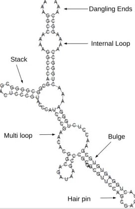
3.3 RNA Structure Prediction . . . 30
3.3.1 The Nussinov Algorithm . . . 31
3.3.2 The Zuker Algorithm . . . 32
3.4 High Performance Bioinformatics . . . 33
3.5 Conclusion . . . 34
4 HLS Based Acceleration: From C to Circuit 35 4.1 Reconfigurable Computing . . . 35
4.2 Accelerators for Biocomputing . . . 38
4.3 High Level Synthesis . . . 39 i
4.3.1 Advantages of HLS over RTL coding . . . 39
4.4 HLS Design Steps . . . 41
4.4.1 Compilation . . . 41
4.4.2 Operation Scheduling . . . 41
4.4.3 Allocation & Binding . . . 47
4.4.4 Generation . . . 50
4.5 High Level Synthesis Tools: An Overview . . . 50
4.5.1 Impulse C . . . 51
4.5.2 Catapult C . . . 52
4.5.3 MMAlpha . . . 53
4.5.4 C2H . . . 54
4.6 Conclusion . . . 54
5 Efficient Hardware Generation with HLS 57 5.1 Bit-Level Transformations . . . 57
5.1.1 Bit-Width Narrowing . . . 58
5.1.2 Bit-level Optimization . . . 59
5.2 Instruction-level transformations . . . 60
5.2.1 Operator Strength Reduction . . . 60
5.2.2 Height Reduction . . . 61 5.2.3 Code Motion . . . 63 5.3 Loop Transformations . . . 65 5.3.1 Unrolling . . . 65 5.3.2 Loop Interchange . . . 66 5.3.3 Loop Shifting . . . 66 5.3.4 Loop Peeling . . . 68 5.3.5 Loop Skewing . . . 68 5.3.6 Loop Fusion . . . 68 5.3.7 C-Slowing . . . 69
5.3.8 Loop Tiling & Strip-mining . . . 70
5.3.9 Memory Splitting & Interleaving . . . 70
5.3.10 Data Replication, Reuse and Scalar Replacement . . . 71
5.3.11 Array Contraction . . . 73
5.3.12 Data Prefetching . . . 73
5.3.13 Memory Duplication . . . 74
5.4 Conclusion . . . 76
6 Extracting Parallelism in HMMER 79 6.1 Introduction . . . 79
6.2 Background . . . 80
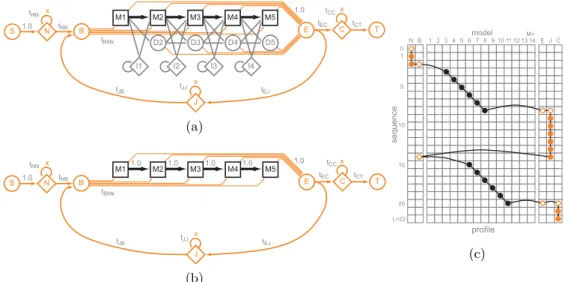
6.2.1 Profile HMMs . . . 80
6.2.3 Look ahead Computations . . . 82
6.3 Related work . . . 83
6.3.1 Early Implementations . . . 83
6.3.2 Speculative Execution of the Viterbi Algorithm . . . 85
6.3.3 GPU Implementations of HMMER . . . 87
6.3.4 HMMER3 and the Multi Ungapped Segment Heuristic . . . 87
6.3.5 Accelerating the Complete HMMER3 Pipeline . . . 89
6.4 Rewriting the MSV Kernel . . . 89
6.5 Rewriting the P7Viterbi Kernel . . . 90
6.5.1 Finding Reductions . . . 91
6.5.2 Impact of the Data-Dependence Graph . . . 93
6.6 Parallel Prefix Networks . . . 94
6.7 Conclusion . . . 96
7 Hardware Mapping of HMMER 97 7.1 Hardware Mapping . . . 98
7.1.1 Architecture with a Single Combinational Datapath . . . 98
7.1.2 A C-slowed Pipelined Datapath . . . 98
7.1.3 Implementing the Max-Prefix Operator . . . 99
7.1.4 Managing Resource Constraints through Tiling . . . 100
7.1.5 Accelerating the Full HMMER Pipeline . . . 101
7.2 Implementation through High-Level Synthesis . . . 102
7.2.1 Loop Transformations . . . 102
7.2.2 Loop Unroll & Memory Partitioning . . . 103
7.2.3 Ping-Pong Memories . . . 103
7.2.4 Scalar Replication . . . 103
7.2.5 Memory Duplication . . . 104
7.3 Experimental results . . . 104
7.3.1 Area/Speed Results for the MSV Filter . . . 104
7.3.2 Area/Speed Results for Max-Prefix Networks . . . 104
7.3.3 Area/Speed Results for the P7Viterbi Filter . . . 105
7.3.4 System level performance . . . 107
7.3.5 A Complete System-Level Redesign . . . 108
7.3.6 Discussion . . . 110
7.4 Conclusion . . . 110
8 Conclusion & Future Perspectives 113 8.1 Conclusion . . . 113
1
Introduction
1.1
High Performance Computing for Bioinformatics
La Bioinformatique est un domaine r´ecent, mais qui suscite depuis une dizaine d’ann´ee de plus en plus d’int´erˆet dans la communaut´e scientifique. Ce domaine recouvre des champs disciplinaires tr`es vari´es incluant la biologie, la g´en´etique, l’informatique mais ´egalement les math´ematiques. L’objectif premier de la bioinformatique est d’offrir aux biologistes des outils informatiques qui leur permettront d’analyser des donn´ees issues de s´equences g´en´etiques (par exemple de l’ADN, de l’ARN et/ou des prot´eines) afin d’essayer de d´ecouvrir ou de pr´edire les fonctions biologiques associ´ees `a ces s´equences.
Les probl´ematiques de la bio-informatique sont nombreuses, parmi celles-ci on peut citer la d´ecouverte de g`enes dans des s´equences d’ADN, la pr´ediction (et la classification) de la structure et des fonctions de prot´eines ainsi que la construction automatique d’arbres phylog´eniques en vue de l’´etude des relations ´evolutives.
En outre, cette derni`ere d´ecennie a vue l’apparition de techniques de s´equen¸cage d’ADN `
a haut d´ebit, qui ont permises de grandes avanc´ees (s´equen¸cage complet du g´enome humain [VAM+01], projet d’annotation du g´enome des plantes [SRV+07]). Ces progr`es se sont `a leur tour traduits par une explosion du volume de donn´ees g´enomiques (ADN, proteines) disponibles pour la communaut´e, comme l’illustre la figure 2.1, qui montre l’´evolution des banques NCBI GenBank [NCB11] (ADN) UniProt [INT] (proteines).
Il est `a noter que les nouvelles g´en´erations de technologies de s´equen¸cage, facilitent encore plus l’extraction d’´enormes quantit´es de s´equences, et vont certainement accentuer cette croissance exponentielle.
Les chercheurs sont de fait d´esormais confront´es `a un d´efi majeur : extraire de ces volumes de donn´ees gigantesques des informations utiles `a la compr´ehension de ph´enom`enes biologiques. Les outils traditionnellement utilis´es par la communaut´e bioinformatique ne sont en effet pas con¸cus pour fonctionner sur de telles masses de donn´ees, et les volumes de calculs mis en jeux dans ces outils d’analyses sont devenus trop importants au point de devenir un goulot d’´etranglement.
0 50 100 150 200 250 300 Bi ll ion s Number of Base Pairs in GenBank (a) (b)
Figure 1.1: The exponential growth of the (a) GenBank and (b) UniPortKB databases [NCB11, ?].
De nombreux travaux se sont donc int´eress´es `a l’utilisation de machines parall`eles pour r´eduire ces temps de calcul. Si les premier travaux ciblaient essentiellement des architectures de super-calculateurs classiques [SRG03, YHK09, CCSV04, GCBT10] (grilles, clusters), la d´emocratisation des architectures multi-cœurs [Edd, LBP+08] et l’´emergence du GPGPU1ont rendu ces travaux plus populaires. Outre ces travaux portant sur des architecture g´en´eralistes programmables, il faut ´egalement mentionner l’utilisation d’acc´el´erateur mat´eriels sp´ecialis´es `a base de logique programmable [HMS+07, SKD06, DQ07, LST] qui a d´emontr´e qu’il ´etait possible de profiter de capacit´es d’acc´el´eration tr`es ´
elev´ees pour tout en restant `a des niveaux de consommation ´electriques et donc des coˆuts de maintenance tr`es raisonnables.
L’augmentation de la densit´e et de la vitesse des circuits FPGA a ainsi favoris´e l’´emergence d’acc´el´erateurs mat´eriels reconfigurables orient´es vers le domaine du calcul haute performance (HPC), avec des applications en calculs financier [ZLH+05, WV08], simulations m´et´eorologiques [AT01], traitements vid´eo [LSK+05] mais ´egalement en bioinformatique[DQ07, SKD06].
Les acc´el´erateurs FPGAs se sont ainsi av´er´es ˆetre des architectures mat´erielles bien adapt´ees `a la mise en œuvre de traitements de type bioinformatique. Ceux-ci offrent souvent la possibilit´e d’exposer un un niveau important de parall´elisme `a grain fin dans l’algorithme, lequel peut ensuite ˆetre exploit´e tr`es efficacement par une mise en œuvre sur FPGA. Une part importante des algorithmes de bioinformatique repose en effet sur l’utilisation de techniques `a base de programmation dynamique, en autre pour la comparaison de s´equence (Smith-Waterman [SW81], Needleman-Wunsch [NW70] and BLAST [AGM+90]), l’alignement multiple de s´equences (CLUSTALW [THG94]), la recherche sur profil (HMMER [Edd]), le repliage de s´equences de RNA (MFOLD [Zuk03]) et mˆeme la construction d’arbres phylog´eniques (PHYLIP [Fel93]). Le caract`ere r´egulier des traitements effectu´es dans ces algorithmes se prˆete ainsi facilement `a une parall´elisation sur un architecture de type r´eseau r´egulier disposant de communication locales.
1
Qui vise `a utiliser les capacit´es de calculs tr`es importantes des cartes graphiques pour acc´el´erer des calculs scientifiques
1.2 – FPGA based Hardware Acceleration 3
1.2
FPGA based Hardware Acceleration
Les circuits FPGAs se pr´esentent comme un gigantesque matrice de cellules logiques programmables, ils peuvent donc ˆetre configur´es pour impl´ementer un nombre ´elev´e de chemins de donn´ees mat´eriels sp´ecialis´es et fonctionnant en parall`ele. Les d´eveloppeurs peuvent ainsi directement impl´ementer un acc´el´erateur mat´eriel d´edi´e `a l’application et tirer parti des gains en performance dus au parall´elisme et `a la sp´ecialisation.
Dans un FPGA, l’expression de ce parall´elisme peut prendre de nombreuses plusieurs formes : parall´elisme de tˆaches en implantant plusieurs cœurs de calculs op´erant en parall`ele, parall´elisme d’op´erations au travers de l’utilisation de chemins de donn´ees pipelin´es complexes. Parce que les FPGAs fonctionnent `a des fr´equences d’horloges bien plus faibles que les processeurs (en moyenne par un facteur 10), ils doivent compenser leur lenteur relative en exploitant un niveau de parall´elisme massif au sein du circuit, tout en s’assurant de la possibilit´e d’alimenter le circuit en donn´ee `a une cadence suffisante.
Une des techniques utilis´ees pour am´eliorer `a la fois le degr´e de parall´elisme et la fr´equence de fonctionnement des circuits implant´es sur le FPGA est d’utiliser des encodages de donn´ees `a pr´ecision r´eduite (entiers `a pr´ecision arbitraire, et codage virgule fixe en lieu et place des flottants).
Ici encore les algorithmes de bioinformatique se prˆetent tr`es bien `a ce genre d’optimisations (par exemple, le codage d’un base ADN peut se faire sur 2 bits au lieu d’un octet complet). Ces caract´eristiques en font donc de tr`es bon candidats `a une acc´el´eration mat´erielle sur FPGA, en particulier compar´e `a des machine de type GPUs plus orient´e vers le calcul flottant. De nombreux travaux se sont donc int´eress´es `a la mise en uvre, sur FPGA, dacc´el´erateur mat´eriels pour les algorithmes les plus couramment utilis´es [HMS+07, SKD06, DQ07].
Ces impl´ementations, qui ont d´emontr´es des facteurs dacc´el´eration tr`es encourageant, se basent sur des sp´ecifications du circuit ´ecrites en VHDL ou Verilog, et tr`es fortement optimis´ees pour une technologie FPGA donn´ee. Ce type dapproche pose de fait des probl`emes de portabilit´e, et passer dun acc´el´erateur FPGA `a un autre n´ecessite souvent de reprendre la conception du circuit `a z´ero. Le section suivante aborde ce probl`eme et discute de la pertinence des outils de synth`ese de haut niveau dans ce contexte.
1.3
FPGA Design Flow
Le flot de conception standard pour circuit FPGA se base en grand partie sur celui d’un ASIC. Les principales ´etapes de ce flot sont repr´esent´ees dans la Figure 2.2a, elles ne concernent cependant que la partie mat´erielle d’un co-design logiciel-mat´eriel, le logiciel embarqu´e ´etant d´evelopp´e `a l’aide de chaˆınes de compilation classiques.
La premi`ere ´etape de ce flot consiste `a d´efinir les sp´ecifications fonctionnelles des composants dans des langages de haut niveau (C, C++, Matlab) afin de d´eterminer le comportement exact du syst`eme. Une fois valid´ee, le concepteur doit d´efinir une
C / C++ / Matlab Specification
Validate Behavioral Model
Define Architecture
Implementation (Vhdl / Verilog)
Verification
Synthesis
Place & Route
FPGA
C / C++ / Matlab Specification
Validate Behavioral Model
HLS Specification
Synthesis
Place & Route
FPGA
(a) C / C++ / Matlab Specification
Validate Behavioral Model
Define Architecture
Implementation (Vhdl / Verilog)
Verification
Synthesis
Place & Route
FPGA
C / C++ / Matlab Specification
Validate Behavioral Model
HLS Specification
Synthesis
Place & Route
FPGA (b)
Figure 1.2: Flot de conception FPGA: (a) Flot de conception traditionnel bas´e sur l’utilisation de langages de description de mat´eriel (HDLs). La description d’une application en HDL est d´elicate et n´ecessite un effeort de v´erifictaion important. (b) Flot de synth`ese bas´e sur l’utilisation d’outils de synth`ese de haut niveau: l’´etape de conception manuelle au niveau RTL est rempla´ee par une description comportementale de haut niveau, suivie d’un phase de g´en´eraion automatique de description RTL.
architecture mat´erielle qui sera en mesure de satisfaire les contraintes de performance, de coˆut et de consommation ´electrique impos´es par le cahier des charges.
Une fois l’architecture d´efinie, les concepteurs doivent d´ecrire cette architecture au niveau RTL (Register to Logic) `a l’aide de langages de description de mat´eriel (Verilog ou VHDL) ou de sp´ecifications sch´ematiques. Cette description est ensuite valid´ee `a l’aide de simulations, afin de garantir sa correction.
Une fois v´erifi´ee, la description du circuit est alors synth´etis´ee, c’est-`a-dire transform´ee en une repr´esentation `a base de primitives logiques du FPGA cibl´e appel´ee netlist. Cette repr´esentation est ensuite plac´ee et rout´ee sur le circuit FPGA cibl´e, en permet de d´eriver un fichier bitstream qui servira `a configurer le FPGA.
Ce flot de conception reste cependant tr`es complexe et n´ecessite souvent de nombreuses it´erations avant d’obtenir une configuration mat´erielle op´erationnelle.
La premi`ere difficult´e est de bien choisir la cible architecturale (type de FPGA, capacit´es de traitement, de m´emorisation, etc.), car celle-ci va conditionner une grande partie des choix de conception ult´erieurs. Un mauvais choix initial peut ainsi avoir un impact tr`es important sur l’effort de conception global. Le seconde (et principale) difficult´e est la sp´ecification au niveau RTL (Register to Logic) de l’architecture de l’acc´el´erateur, qui se fait `a l’aide de langage de description mat´eriel tels VHDL ou Verilog. Cette ´etape est tr`es fastidieuse et n´ecessite une ´etape de d´ebogage tr`es longue, avec de nombreuses it´erations entre les ´etapes de sp´ecification et de validation.
1.3 – FPGA Design Flow 5
La complexit´e toujours croissante des syst`emes ´electroniques, qui s’illustre par une constante augmentation des fonctionnalit´es int´egr´ees sur un seul circuit FPGA, rend cette ´etape de conception RTL de plus en plus critique [CD08]. De fait, les outils de conceptions utilis´es pour la mise en œuvre de syst`emes de communication sans-fils 4G sont les mˆeme que pour le standard GSM, et ce malgr´e l’´enorme ´ecart de complexit´e entre ces deux standards.
De nombreux travaux se sont donc int´eress´es `a ce probl`eme, en proposant de relever le niveau d’abstraction utilis´e la sp´ecification de composants. L’objectif est d’offrir des outils de g´en´eration automatique de description RTL `a partir de sp´ecification algorithmiques dans des langages de plus haut niveau tel C ou SystemC. On parle alors d’outils de synth`ese de haut niveau.
1.3.1 Synth`ese de haut niveau
Les outils de synth`ese de haut niveau (High Level Synthesis) visent principalement `a r´eduire les d´elais de conception, en utilisant des sp´ecifications de plus haut-niveau que celles offertes par les approches bas´es sur des descriptions RTL. En plus de r´eduire le temps de conception `a proprement parler, les outils d’HLS permettent ´egalement de fortement r´eduire le temps de v´erification, en diminuant le nombre d’it´eration n´ecessaire pour obtenir un composant fonctionnel. Par ailleurs en lib´erant le concepteur de la gestion des horloges, du partage de ressource et de l’interfa¸cage m´emoire, ces outils r´eduisent ´egalement les risques d’erreurs.
Le portage de sp´ecification RTL d’une technologie `a une autre se fait souvent au prix d’une baisse des performances et d’une augmentation du coˆut en ressource et en consommation ´energ´etique [Fin10].
Au contraire, parce que la sp´ecification HLS se fait au niveau fonctionnel, le portage d’une IP mat´erielle d’une plate-forme `a une autre est simplifi´e, puisque c’est l’outil d’HLS qui va se charger de r´ealiser le mapping technologique.
Pour autant, les architectures mat´erielles g´en´er´ees automatiquement `a partir d’un niveau de sp´ecification plus abstrait ne sont que rarement aussi efficaces que des impl´ementations manuelles. En cons´equence, les faibles performances obtenues par une utilisation na¨ıve de ces outils limitent l’int´erˆet des FPGAs dans un contexte de calcul
haute performance .
Ces faibles performances s’expliquent par l’incapacit´e de ces outils `a extraire un niveau de parall´elisme suffisamment ´elev´e. Les acc´el´erateurs mat´eriels issus de ces outils peinent de fait `a rivaliser avec des architecture GPU et multi-cœurs, et ce d’autant plus qu’il doivent compter sur une fr´equence de fonctionnement plus faible.
Il est possible de lever cette difficult´e, en modifiant directement le code source de l’application de mani`ere `a faire apparaˆıtre un niveau de parall´elisme qui sera exploitable par l’outil. Ce type de technique est tr`es efficace d`es lors que l’on cherche `a acc´el´erer des calculs r´eguliers, ayant la forme de nids de boucles. En effet, il est possible de d’appuyer sur la grande quantit´e de travaux issus de la communaut´e de parall´elisation
6 Introduction s3 s2 s5 s4 s7 s6 s9 s8 s11 s10 s13 s12 s15 s14 s1 s0 x3 x2 x5 x4 x7 x6 x9 x8 x11 x10 x13 x12 x15 x14 x1 x0 s (a) x3 x2 x5 x4 x7 x6 x9 x8 x11 x10 x13 x12 x15x14 x1 x0 s3 s2 s5 s4 s7 s6 s9 s8 s11 s10 s13 s12 s15 s14 s1 s0 x3 x2 x5 x4 x7 x6 x9 x8 x11 x10 x13 x12 x15 x14 x1 x0 s (b)
Figure 1.3: Examples of Reduction, (a), and Scan, (b), are shown here, with a possible order of computation.
automatique [Wol90, Wol96].
Outre les aspects li´es `a la parall´elisation des calculs proprement dits, l’obtention de bonne performances n´ecessite ´egalement de prendre en compte de mani`ere tr`es fine la gestion des donn´ees dans les diff´erents niveaux de hi´erarchie m´emoire du syst`eme (m´emoire hˆote, m´emoire locale sur la carte, m´emoire embarqu´ee). Une des contributions de ce travail est de pr´esenter une revue d’ensemble des transformations cl´es permettant d’obtenir, grˆace `
a des outils de synth`ese de haut niveau, des architectures mat´erielles sp´ecialis´ees exploitant efficacement les possibilit´es des acc´el´erateurs FPGAs actuels.
1.4
Parall´
elisation `
a l’aide de r´
eductions et de pr´
efixes
parall`
eles
Les algorithmes ´el´ementaires utilis´es en alg`ebre lin´eaire peuvent ˆetre class´es en deux cat´egories. Dans la premi`ere, la taille du r´esultat d’un calcul est du mˆeme ordre que la taille de ces op´erandes; c’est par exemple le cas de l’addition de deux vecteurs. Dans la seconde la taille du r´esultat est plus beaucoup plus petite (en g´en´eral une valeur scalaire), d’o`u le terme de r´eduction propos´e par Iverson [Ive62], et qui correspond par exemple `a l’op´eration de sommation des ´el´ements d’un vecteur ou d’une matrice.
Dans ce travail, nous nous sommes int´eress´es `a deux types de calculs : les op´erations de r´eduction et les op´erations de pr´efixes2. Ces op´erations, qui op`erent sur des collections d’objets, sont bas´ees sur l’utilisation d’un op´erateur ´el´ementaire disposant de propri´et´es de commutativit´e et d’associativit´e.
Soit ⊕ le symbole identifiant cet op´erateur ´el´ementaire, une r´eduction sur un vecteur
1.5 – Contributions de cette th`ese 7
op´erande (x1, x2, . . . , xn) s’´ecrit comme:
s = n M
i=0
xi =x0⊕ x1⊕ . . . ⊕ xn (1.1)
Pour l’op´eration de pr´efixe, la taille du r´esultat est la mˆeme que celle de l’op´erande, et se d´efinit, pour vecteur op´erande (x1, x2, . . . , xn) et pour un vecteur r´esultat (s1, s2, . . . , sn) comme: sk= k M i=0 xi =x0⊕ x1⊕ . . . ⊕ xk (1.2)
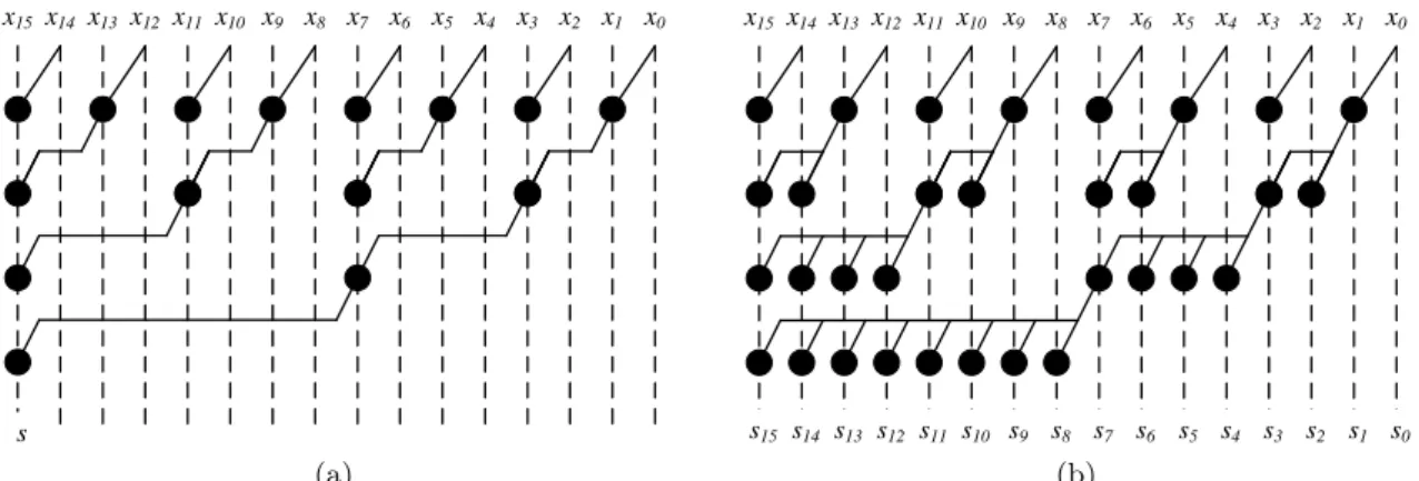
Ces deux types d’op´erations sont repr´esent´ees sur la Figure 2.3 pour n = 16. Il est important de remarquer que ces op´erations, a priori s´equentielles dans leur d´efinition, peuvent ˆetre r´ealis´ees de mani`ere parall`ele en r´eorganisant les calculs de mani`ere plus ou moins complexe. En particulier, la mise en œuvre efficace d’op´erations de type pr´efixes sur circuits VLSI est un sujet qui a re¸cu beaucoup d’attention3, et ce depuis le d´ebut des ann´ees 60. De nombreuses structures mat´erielles permettant d’explorer des compromis entre rapidit´e et coˆut en surface ont ainsi ´et´e propos´ees [LF80, BK82, KS73, HC87, Skl60]. La mise en œuvre mat´erielle d’un algorithme utilisant des op´erations de pr´efixes peut profiter de ces r´esultats, en explorant les diff´erentes possibilit´es de r´ealiser le traitement pour choisir la plus efficace. Cette exploration est d’autant plus facile lorsque la conception se fait `a haut niveau d’abstraction, par exemple en utilisant des outils de synth`ese de haut niveau.
Les algorithmes d’alignement de s´equences utilis´es en bioinformatique, sont bas´es sur des algorithmes de programmation dynamique, et exposent des sch´emas de calcul se prˆetant justement assez bien `a des reformulations math´ematiques permettant de faire ressortir des op´erations de r´eductions et/ou de pr´efixe.
Dans le chapitre ??, nous montrons comment certains des traitements mis en jeu dans l’outil HMMER [Edd] peuvent ˆetre reformul´ees comme des op´erations de r´eductions et/ou de pr´efixes, lesquelles permettent une parall´elisation plus efficace.
1.5
Contributions de cette th`
ese
Le chapitre 3 propose une courte introduction au domaine de la bioinformatique, et `a ses enjeux. Nous d´etaillons en particulier les principaux algorithmes utilis´es pour l’alignement la comparaison et le repliement de s´equences, en mettant l’accent sur leur coˆut en termes de traitements et sur leur capacit´e `a passer `a l’´echelle sur de gros volumes de donn´ees. Nous montrons en particulier que la plupart des approches utilis´es ne passent pas `a l’´echelle, et n´ecessitent de recourir `a des architectures mat´erielle exploitant des niveaux de parall´elisme important.
Le chapitre 4 pr´esente ensuite un survol des techniques et outils de synth`ese de haut niveau. Ces outils permettent de d´eriver une architecture mat´erielle sp´ecialis´ee directement `a partir d’une sp´ecification algorithmique (par exemple en C). Ils permettent ainsi de r´eduire de mani`ere drastique les temps de conception. Le chapitre pr´esente les diff´erentes ´etapes mises en jeu dans un flot de synth`ese HLS, et propose un ´etat de l’art des techniques utilis´ees dans ces outils. Le chapitre se termine par une revue des outils de HLS acad´emiques et commerciaux actuellement disponibles.
Le chapitre 5 s’int´eresse quant `a lui aux techniques de transformation de code permettant d’am´eliorer les performances des architectures obtenues par synth`ese HLS. Cette partie du manuscrit s’int´eresse en particulier aux transformations de boucles pour la parall´elisation et `a l’optimisation des acc`es `a la m´emoire, qui sont des points cruciaux pour l’obtention d’acc´el´erateurs efficaces.
Les chapitres 6 & 7 pr´esentent quant `a eux les contributions de ce travail, qui portent sur l’utilisation de transformations de programme complexes, en vue de l’acc´el´eration mat´eriel du programme HMMER. Cet outil, tr`es utilis´e dans la communaut´e bioinforma-tique, repose sur deux noyaux de calculs (MSV et P7Viterbi) r´eput´es difficiles `a acc´el´erer du fait de la pr´esence de d´ependances de donn´ees qui empˆechent a priori toute parall´elisation. Dans le chapitre 6, nous pr´esentons l’´etat de l’art concernant la parall´elisation de HMMER sur FPGA et proposons une reformulation des noyaux MSV et P7Viterbi qui permet de mettre en ´evidence un niveau important de parall´elisme au travers d’op´erations de r´eductions et de pr´efixes.
Le chapitre 7 s’int´eresse quand `a lui `a la mise en œuvre, sur un acc´el´erateur FPGA et `a l’aide d’un outil HLS commercial, d’une architecture de co-processeur parall`ele pour HMMER. L’originalit´e de l’approche vient de l’utilisation d’un sch´ema de calcul complexe, exploitant du parall´elisme `a grain fin (boucles vectoris´ees) et `a gros grain (utilisation d’un macro-pipeline de tˆache). Ces sch´emas ont donn´es lieu `a une mise en œuvre mat´erielle sur une carte FPGA (XtremeData), et nous a permis de d´emontrer des facteur d’acc´el´eration int´eressant par rapport `a une mise en œuvre optimis´ee exploitant de mani`ere tr`es fine les extension SIMD des processeurs multi-cœurs Intel.
2
Introduction
2.1
High Performance Computing for Bioinformatics
Bioinformatics can be defined as an application of concepts from computer science, mathematics and statistics to analyze biological data (e.g. DNA, RNA and Proteins) and to predict their the functions and structures. The typical problems found in bioinformatics consist in finding genes in DNA sequences, analyzing new proteins, aligning similar proteins into families and generating phylogenetic trees to expose evolutionary relationships.
In the last decade, there has been a rapid growth in the amount of available digital biological data with the advancement in DNA sequencing techniques, and particularly the success of projects such as The Human Genome Project [VAM+01] and genome annotation projects for plants [SRV+07]. The noticeable examples are the growth of DNA sequence information in NCBI’s GenBank [NCB11] database and the growth of protein sequences in the UniProt [?] database, as shown in Figure 2.1. Furthermore, the next-generation sequencing technologies have enabled the extraction of genome sequence data in huge quantities, and this will result in further growth of these databases.
Computer scientists and biomedical researchers are now facing a major challenge of transforming this enormous amount of genomic data into biological understanding. The traditional tools and algorithms in bioinformatics were designed to handle very small databases, hence a bottleneck in terms of computational time has arisen when scaled up to facilitate analyses of large data-sets and databases. Recently, a lot of research efforts have been done enabling modern bioinformatics tools to take advantage of parallel computing environments. The implementation of bioinformatic applications on modern multicore general-purpose processors [Edd, LBP+08], General Purpose Graphic Processors (GPGPU) [WBKC09b, VS11, MV08], grid technology [SRG03, YHK09, CCSV04, GCBT10] and reconfigurable platforms, such as field-programmable gate arrays (FPGAs) [HMS+07, SKD06, DQ07, LST] have shown promising acceleration and have significantly reduced the runtime of many biological algorithms while operating on the
0 50 100 150 200 250 300 Bi ll ion s Number of Base Pairs in GenBank (a) (b)
Figure 2.1: The exponential growth of the (a) GenBank and (b) UniPortKB databases [NCB11, ?].
enormous databases.
The considerable increase in logic density and clock speed of FPGAs, in recent years, have in turn increased the trend of using FPGAs to implement compute intensive algo-rithms from various domains, including finance [ZLH+05, WV08], weather forecast [AT01], video encoding [LSK+05] and bioinformatics[DQ07, SKD06]. FPGAs are an attractive target architecture for bioinformatics applications, considering their cost-effectiveness as customized accelerators and their ability to exploit the fine-grain parallelism available in many bioinformatics applications. A large class of bioinformatics applications rely on dynamic programming algorithms or a fast approximation of one, including sequence database search programs (Smith-Waterman [SW81], Needleman-Wunsch [NW70] and BLAST [AGM+90]), multiple sequence alignment programs (CLUSTALW [THG94]), profile based search programs (HMMER [Edd]), RNA-folding programs (MFOLD [Zuk03]) and even phylogenetic inference programs (PHYLIP [Fel93]). The FPGA architecture is very well suited for such dynamic programming algorithms, since it has a regular structure, similar to the data dependencies in dynamic programming algorithms, with a communication network to close neighbors.
2.2
FPGA based Hardware Acceleration
FPGAs are simply large fields of programmable gates, so they can be programmed into many parallel hardware execution paths. Due to their parallel nature, different processing operations do not have to compete for the same resources. The designer can map any number of task-specific cores on an FPGA, that all run as simultaneous parallel circuits.
On an FPGA, a designer can exhibit parallelism with the help of a variety of computation granularities (i.e. fine and coarse-grain parallelism), pipelining the long computation paths and through data parallelism. The parallelism granularity may range from very fine-grain computations (e.g. bit-level operations), to fine-grain operations, as in a SIMD architecture (e.g. word- and instruction-level operations) and to coarse-grain computations (e.g. many independent instances of a highly compute intensive kernel,
2.3 – FPGA Design Flow 11
operating in parallel).
Since FPGAs operate on a very low frequency (about 10 × low) in comparison with a CPU, so in order to outperform the CPU based performance, there should be enough computations to be computed in parallel. Hence compute intensive applications with massive inherent parallelism (e.g. converting each pixel of a color image to grayscale) are highly suitable for FPGA based implementation. Similarly applications with reduced width data are appropriate for FPGAs, due to their ability to compute custom bit-width operations. The majority of bioinformatics algorithms do not require even the full integer precision, thus floating point arithmetic on a modern CPUs will be not valuable. Therefore, FPGA based implementation of such applications can exploit the customizable precision and parallelism, and can result in improved speed and better utilization of the available resources.
The properties held by bioinformatic applications make them viable for FPGA based acceleration in comparison with other acceleration approaches, such as clusters and GPUs. And a lot of research work has been done to accelerate these applications on FPGAs using traditional hardware languages (VHDL and Verilog) [HMS+07, SKD06, DQ07]. The resulting implementations are very efficient and the obtained speedup is highly valuable. However, there are few issues with FPGA based implementations that hinders the designer to opt for an FPGA based implementation, e.g. the design flow is highly error prone and lengthy verification phase often becomes the bottleneck in design projects. In next section, we will highlight these issues by discussing the traditional FPGA design flow and a possible solution to these issues through high-level synthesis.
2.3
FPGA Design Flow
The standard design flow for FPGA designs is borrowed from ASICs, as shown in Figure 2.2a. In practice, a design is usually partitioned into hardware & software parts. The steps shown in Figure 2.2a are related only to the implementation of hardware blocks in such a design, while the software blocks will be implemented using standard software development techniques.
The first step in design flow is to define functional specifications in C, C++, Matlab or any other language in order to validate and fine-tune the desired behavior. Once tested, the designer needs to define an optimal architecture to implement the desired functionality. The architecture selection defines the performance, area and power consumption goals to be met. After the architecture is defined, the design team hand-codes these decisions in the form of a Hardware Description language (Verilog or Vhdl) or in the form of a schematic design. At this stage, functional simulation is carried out to verify the correctness of the described functionality.
After functional verification, the design can be synthesized, i.e. mapping boolean operators on lookup tables (LUTs) modules, shown in Figure 4.1b. The result of logic synthesis is called the netlist, a file describing the modules to be used for the
C / C++ / Matlab Specification
Validate Behavioral Model
Define Architecture
Implementation (Vhdl / Verilog)
Verification
Synthesis
Place & Route
FPGA
C / C++ / Matlab Specification
Validate Behavioral Model
HLS Specification
Synthesis
Place & Route
FPGA
(a) C / C++ / Matlab Specification
Validate Behavioral Model
Define Architecture
Implementation (Vhdl / Verilog)
Verification
Synthesis
Place & Route
FPGA
C / C++ / Matlab Specification
Validate Behavioral Model
HLS Specification
Synthesis
Place & Route
FPGA (b)
Figure 2.2: FPGA Design Flow: (a) Traditional FPGA design flow using Hardware Description languages (HDLs). The application description in HDL is very error prone and requires a lot of verification efforts. Similarly, it is not easy to port design to other FPGA architectures. (b) High-level Synthesis based FPGA design flow: The manual RTL based design steps are replaced with high-level behavioral description of design following by an automatic generation of RTL design.
implementation of the design and its interconnections. In next step, we place and route the design on FPGA, i.e. the operators (LUTs, Flip-Flops, Multiplexers, etc. ) described in the netlist will be now placed on the FPGA fabric and will be connected together through routing. This step is normally done by the CAD tool provided by the FPGA vendor. The CAD tool generates a file called bitstream. The bitstream file contains the description of all the bits to be configured, in order to configure LUTs, the interconnect matrices, multiplexers and I/O of the FPGA. Now, by loading the bitstream file on the FPGA, the hardware will be configured according to the functional specifications of the application.
However, the design flow is not that straightforward and often involves a lot of iterative development steps. First problem is to find a suitable architecture, since the following design steps closely related to the selected architecture. An inadequate choice of underlying architecture will prolong the development cycle greatly. The biggest problem in the design flow is the manual RTL description, as when the design is tested after first implementation, bugs are reported and a lot of development time is usually spent in hunting down and fixing the bugs individually. The iterative process of fixing bugs, generating new bugs and fixing them again, prolongs the time-to-market.
One major issue with HDL based implementation is the ever-increasing complexity of electronic designs. The increase in device capacity only exacerbates this issue, as pro-grammers seek to map increasingly complex computations to even larger devices [CD08]. The reality is that we are trying to develop 4G broadband modems and H264 decoders
2.3 – FPGA Design Flow 13
with tools and methods inherited from era, when GSM and VGA controllers were popular technologies [Fin10]. Eventually, creating RTL design triggers bug and cause the verification phase to be the bottleneck of any ASIC project.
Many research efforts have been done to ameliorate this issue by offering higher-level programming abstractions combined with an automatic RTL generation from popular high-level languages such as C or Matlab, known as High-level Synthesis (HLS) tools. 2.3.1 High-level Synthesis
High-level synthesis addresses the root cause of the problem, posed by HDL based design flow, by providing an error-free path from abstract specification to RTL. HLS reduces the implementation time, while also reduces the overall verification effort. The high-level of abstraction needs a lot less detail for the description, and the designer can only focus on describing the desired behavior. With fewer lines of code, when there are no such details as clocks, technology or micro-architecture specifications in side the sources, the risk of errors is greatly reduced. Similarly with fewer blocks to verify, the design can be exhaustively verified.
The abstract functional specifications in HLS, makes the design reuse more effective. Since the design sources are now the abstract specification of the design, retargeting to other architectures is easier. Similarly, the concepts of IP and reuse, which have been promoted to address the design complexity challenge with RTL design, are often unhelpful. The retargeting of legacy RTL is usually done at the expense of power, performance and area [Fin10]. However, in HLS, we are dealing with pure functional specifications and technology specific information is added later by HLS tool automatically. This makes the IP reuse and change in existing functionality, easy to implement and verify.
For biocomputing applications, HLS framework simplify the complex algorithmic description phase and also maximize the design portability. However, the abstract specification of a design may lack several design optimization details, which also expands the hardware mapping possibilities. This can lead to a less efficient design through automatic RTL design generation, in comparison with the efficiency of a highly detailed manual RTL design. Consequently, the resulting performance of HLS based design is often not good enough to justify the use of an FPGA based acceleration. Most of the research efforts in development of these HLS tools, are dedicated to an efficient translation of the given input C code into a hardware design, and this task has been accomplished quite effectively. However, there has been a very little focus on automatic parallelization extraction from the input C code. Therefore, the designer needs to pay a lot of attention on ‘what’ kind of C code will generate ‘what’ kind of circuit.
To tackle this problem, the HLS input needs to be reformed by exposing the hidden parallelism in the algorithm. This task can be accomplished with a prior dependency analysis of input design and based on this analysis parallelism can be expressed with the help of modern high performance compiler optimization techniques [Wol90, Wol96]. The input code should also manage memory resources in an efficient way ( i.e. minimizing
14 Introduction s3 s2 s5 s4 s7 s6 s9 s8 s11 s10 s13 s12 s15 s14 s1 s0 x3 x2 x5 x4 x7 x6 x9 x8 x11 x10 x13 x12 x15 x14 x1 x0 s (a) x3 x2 x5 x4 x7 x6 x9 x8 x11 x10 x13 x12 x15x14 x1 x0 s3 s2 s5 s4 s7 s6 s9 s8 s11 s10 s13 s12 s15 s14 s1 s0 x3 x2 x5 x4 x7 x6 x9 x8 x11 x10 x13 x12 x15 x14 x1 x0 s (b)
Figure 2.3: Examples of Reduction, (a), and Scan, (b), are shown here, with a possible order of computation.
data communication overhead and maximizing data reuse). Hence, there is a dire need to identify, analyze and layout the rules and guidelines, a designer should keep in mind, while designing for hardware using high-level synthesis tools.
The leitmotiv of this thesis consists in a critical analysis of state of the art HLS tools, identifying their capabilities and shortcomings, formalize techniques to craft an efficient hardware using these tools and exercise these strategies on a well-known, compute-intensive and naively sequential bioinformatic application (i.e. HMMER).
2.4
Exploiting Parallelism with Reductions and Prefixes
The basic algorithms of linear algebra and matrix computation fall into two broad classes. In the first one, the output of a computation is of the same size or bigger than the input data. This is the case, for instance, for vector operations. In the second class, the output is much smaller, typically only one value, than the input data, hence the name reduction which has been coined by Iverson [Ive62].Here, we are interested in two special kind of such computations, namely reduction and scans or prefix computations, where operations hold associativity and commutative properties. Let say, ⊕ represents such an operation, then a reduction can be defined, over a input vector (x1, x2, . . . , xn), as:
s = n M
i=0
xi =x0⊕ x1⊕ . . . ⊕ xn (2.1)
A prefix operation belongs to the first class of computations, where output is exactly the same size as the input, and can be defined for an output vector (s1, s2, . . . , sn) as:
sk = k M
i=0
2.5 – Contributions of this work 15
The operations can be visualized in Figure 2.3 for n = 16. The possibility to compute these operations in parallel and in numerous order of executions, has given significant importance to these computations. While targeting FPGA, a designer can easily devise a compromise between the speed and area.
The parallel implementation of prefix networks (Parallel Prefix) has received a wealth of attention from VLSI community going back almost 50 years and various network topologies have been proposed [LF80, BK82, KS73, HC87, Skl60]. These network topologies allow a variety of hardware implementations of a prefix operation, managing various design trade-offs, such as speed, area, wiring and fan-out. Thus, expressing parallelism in the form of prefix operations allows to utilize these previously developed network topologies. Furthermore, the high-level synthesis based implementation of such networks simplifies the design exploration task.
Sequence alignment techniques, based on dynamic programming algorithms, in bioinformatic applications generally compute a best score for a comparison and the computations involved usually hold the above mentioned algebraic properties. So there is a strong tendency that reduction and prefix computations can be detected in these algorithms and it will lead to parallel implementation of the algorithms. In Chapter ??, we demonstrate how algorithmic dependencies in HMMER [Edd] can be transformed into reductions and prefixes through algorithmic rewriting and which ultimately help to accelerate the execution.
2.5
Contributions of this work
Chapter 3 provides an brief introduction to bioinformatics field and common practices in this field. We highlight some important algorithms for sequence alignment and RNA folding. A review of these algorithms provides a fair insight to the algorithmic complexities and also highlights the challenge being faced by biologists and computer scientists, i.e. exercising these algorithms on constantly growing size of genome databases in becoming time prohibitive. There is a pressing need to utilize the advancements in computation platforms and accelerate bioinformatics applications.
Chapter 4 discusses how bioinformatics applications are viable for FPGA based acceleration. It also reasons the importance of high-level synthesis in FPGA based implementation, in comparison with traditional RTL based designs. The chapter introduces to the design flow inside an HLS tool and discusses the state of the art techniques applied in each step of the design flow. It also provides an overview of few well-known HLS tools in market, investigates their handling of input code and identify the basis of performance degradation.
Chapter 5 is dedicated to design techniques and code transformations, a designer needs to bear in mind while designing hardware from high-level specifications (i.e. C code). The sole idea is to highlight that ‘what’ kind of C code will be translated to ‘what’ kind of hardware, and ‘what’ kind of transformations may help to accomplish design goals
(Speed/Area).
Chapter 6 & 7 presents the research work carried out to accelerate HMMER application by exercising the previously discussed techniques for efficient hardware design using HLS. HMMER is a widely usied tool in bioinformatics for sequence homology searching. The computation kernels of HMMER, namely MSV and P7Viterbi are very compute-intensive, and their data dependencies, if interpreted naively, lead to a purely sequential execution. We propose an original parallelization scheme for HMMER based on rewriting its mathematical formulation, in order to expose hidden potential parallelization opportunities by transforming computations into well-known architectures, i.e.parallel prefix networks & reduction trees. Besides exploring fine-grain parallelization possibilities, we employ and compare coarse-grain parallelization through different system-level implementations of the complete execution pipeline, based on either several independent pipelines or a large aggregated pipeline. We implement our parllelization scheme on FPGA, and then present and compare our speedup with the latest HMMER3 SSE version on a Quad-core Intel Xeon machine. Our results show that a careful HLS based implementation can fairly compete an RTL based design in terms of performance and holds a definite edge in terms of time-to-market and design efforts.
3
An Introduction to
Bioinformatics Algorithms
Bioinformatics can be defined as the science of developing computer systems and algorithms for the purpose of spreading up and enhancing biological research [Aga08]. To understand bioinformatics in a meaningful way, it is necessary for a computer scientist to understand some basic biology. This chapter provides a short introduction to those fundamental concepts in biology and highlights some common algorithms being used in bioinformatics.
3.1
DNA, RNA & Proteins:
Cells are the smallest structural unit of life that has all the basic characteristics of a living organism, such as maintaining life and reproducing it [SEQb]. A cell contains all the necessary information as well as the required equipment to not only produce a replica of itself, but also helps its offspring start functioning [JP04]. Each cell in a human body contains 23 pairs of chromosomes, consisting of 30,000 genes in each of them. There are around 1012 cells in a body, which gives an estimate of approximately 3 billion pairs of DNA bases [oEGP08]. Similarly, the plant genome-sequencing project reports more than 40,000 genes in average plants [SRV+07].
The three primary types of molecules studied by biologists are DNA, RNA and proteins. The relationship between these molecules is the transfer of information from DNA to proteins through RNA, as shown in Figure 3.1. DNA encodes RNA that produces the proteins, where proteins are responsible for managing and performing different biological processes inside the cell. A DNA within a cell holds the complete information describing the functionality of the cell. RNA transfers short pieces of this information to different places within the cell, where this information is used to produce proteins [JP04].
DNA is a long molecule forming a chain, where the links of the chain are pieces called 17
Transcription Translation
DNA mRNA
Protein
Figure 3.1: The relationship between DNA, RNA and Proteins is refereed as the central dogma of life. [Courtesy of NIGMS Image Gallery [Gal]]
nucleotides, or ‘bases’, named ‘A’, ‘C’, ‘G’ and ‘T’. DNA encodes the information necessary to build a cell. Most of the cell activities, e.g. breaking down the food as enzymes, building new cell fragments, cell signaling and signal transduction, are carried out by proteins. However, a DNA sequence must be decoded to make a protein and the decoding process requires the creations of an RNA template [Wil03]. The creation of “messenger RNA” or mRNA is called transcription, while the process of creating proteins from the mRNA is called translation.
The discovery of DNA is probably the most influential discovery of the 20th century, that led to extraordinary breakthroughs in the field of science and medicine. The discovery of DNA has enabled the identification of genes, diagnosing of diseases and developing treatments for them.
Why Bioinformatics?
The information that biologists have collected about gene sequences needs to be processed, in order to completely understand their function and roles, e.g. how a specific gene is related to a specific disease, or what are the functions of thousands of proteins and how proteins can be classified, in accordance to the functionalities. The field of Bioinformatics is a collection of such tools and methods that are used to collect, store, analyze and classify this huge amount of biological data.
As mentioned by Thampi [Tha09] regarding the history of bioninformatics, it began in the 1960s with the efforts of Margaret O. Dayhoff, Walter M. Fitch, Russell F. Doolittle and others. Since then it has evolved into a much developed discipline, having strong infulence on modern biology research. In 1970, Saul B. Needleman and Christian D. Wunsch [NW70], proposed the first DNA sequence matching algorithm. However, during the 1990s few major steps brought revolution in bioinformatics study, e.g. the start of
3.2 – Sequence Alignment 19
Figure 3.2: An example for multiple sequence alignment: The region of convergence is the shaded part where exact matches are found in all sequences.
Human Genome Project Bioinformatics, the availability of new analysis, services and the availability of data through Internet. Huge databases, such as GenBank and EMBL were designed to store, compare and analyze the biological sequence data that is being produced at an enormous rate. Today, bioinformatics field involves structural and functional analysis of proteins and genes, drug development and pre-clinical and clinical trials [Tha09].
The field of bioinformatic encompasses the use of tools and techniques from three separate disciplines; the source of the data to be analyzed is related to molecular biology, the platform and resources to analyze this data are borrowed from computer science, and the techniques and tools that analyze this data are based on data analysis algorithms [Ric]. The common activities in bioinformatics are hence storing DNA and protein sequences, analyzing, aligning or comparing, classifying protein families and finding new members, predicting structures of RNAs and constructing phylogenetic trees or evolutionary trees. In this chapter, we will focus on algorithms related to general sequence alignments [NW70, SW81, AGM+90, THG94, Edd11a] and RNA folding [NPGK78, ZS81].
3.2
Sequence Alignment
Sequence alignment is an arrangement of two sequences which shows where the two sequences are similar, and where they differ. Sequence alignment techniques are used to discover structural and functional properties of the biological data and characterizing evolutionary relationship in sequences. The identical characters are identified as matches, while nonidentical characters are mentioned as gaps. The regions with identical characters are known as conserved region, as shown in Figure 3.2. To discover this information it is important to obtain the “optimal” alignment, which is the one that exhibits the most significant similarities, and the fewer differences.
A similarity between two sequences suggests a similarity in the function or the structure of these sequences. Additionally, strong similarities between two sequences may also show the evolutionary relationship between them, assuming that there might be a common ancestor sequence. The alignment indicates the changes that could have occurred between the two homologous sequences w.r.t. a common ancestor sequence during evolution.
There are two types of sequence alignments: global alignments try to align the sequences from end to end for each sequence. Sequences that are similar and that are
approximately the same length are suitable candidates for global alignment. On the contrary local alignments search for segments of the two sequences that are similar. Local Alignment does not force the entire sequence into alignment, instead it only aligns the regions with the highest density of matches. It hence generates one or more sub-alignments in the aligned sequences. Local alignments are more suitable for aligning sequences which are different in length, or sequences that have a strong conserved region but not located at same position in both sequences.
In the following section we will show a comparison of both type of alignments and how for the same sequence pair, alignment result can differ.
Sequences are usually either aligned in pairwise manner, i.e. through a Pairwise sequence alignment, to compare and identify similarities in two sequences. In some other cases, three or more sequences are aligned, i.e. through a Multiple sequence alignment. The latter ones are used to show similarities conserved by most of the sequences and to construct families of these sequences. New members of such families can then be found by searching sequence databases for other sequences exhibiting these same conserved regions.
3.2.1 Pairwise Sequence Alignment
Pairwise alignment methods are used to find optimal local or global alignment of two query sequences. The most common methods for pairwise alignment are dot matrix, dynamic programming and word or k-tuple methods. The most famous dynamic pro-gramming algorithms for pairwise alignment are Smith-Waterman [SW81] and Needleman-Wunsch [NW70] algorithms. BLAST [AGM+90], one of the most widely used bioinformatic tool, is based on a word method.
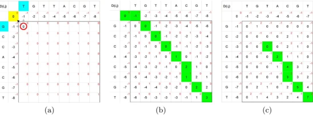
Needleman-Wunsch: Needleman-Wunsch algorithm performs global alignment for a pair of sequences. The algorithm was proposed in 1970 by Saul B. Needleman and Christian D. Wunsch [NW70], and was the first application of dynamic programming to biological sequence comparison. To find the alignment with the highest score, a two-dimensional array (or matrix) D is allocated. The entry in row i and column j is denoted by Di,j. There is one column for each character in sequence A, and one row for each character in sequence B. Each cell of matrix D will be computed using following formula:
Di,j = max Di−1,j−1+δ(Ai, Bj) Di−1,j+δ(Ai, −) Di,j−1+δ(−, Bj) (3.1)
Figure 3.3a shows the initialized matrix and the data dependency, as depicted by the formula above. The numbers in small font, in first row and first column mentions the gap penalty while in rest of the matrix they shows the matching and penalty scores. The matching score, δ(Ai, Bj) is equal to 1 when Ai and Bj are same characters. Otherwise, the penalty is set to 0 for any mismatch. Figre 3.3b shows the global alignment from
3.2 – Sequence Alignment 21
(a) (b) (c)
Figure 3.3: Pair-wise Sequence Alignment: (a) Matrix initialization & computation dependencies , (b) Global alignment with Needleman-Wunsch, (c) Local alignment with Smith-Waterman. The green trail in (b) and (c) shows the alignment. [Figures generated using Basic-Algorithms-of-Bioinformatics Applet [Cas]]
Needleman-Wunsch algorithm. The final alignment for this example:
- G C C A C C G T
| | | | |
T G T T A C - G T
Smith-Waterman: The Smith-Waterman algorithm, also based on dynamic program-ming techniques, computes the optimal local alignment of two sequences. Instead of looking at the entire sequence length, the Smith-Waterman algorithm compares only segments (for all possible lengths) of the input sequences and try to optimizes the similarity score. The main difference with Needleman-Wunsch is that Needleman-Wunsch allows negative scoring, whereas Smith-Waterman forces negative values to zero. This choice of positive scoring makes local alignment visible. The Smith-Waterman algoritm computes the matrixD as:
Di,j = max Di−1,j−1+δ(Ai, Bj) Di−1,j+δ(Ai, −) Di,j−1+δ(−, Bj) 0 (3.2)
Figure 3.3c shows the local alignment, where matching score, δ(Ai, Bj) is set to 2 and all penalties are set to -1. The final alignment in this case is:
A C C G T
| | | |
A C - G T
Local vs. Global Alignment: From the above two alignments, it can be seen that global alignment can align even less conserved regions in comparison with local alignment that only aligns the regions that are well conserved by the two sequences. Similarly, local
CAG - TTATGTGGGCCCAAATTG Global Alignment | | | | | | | GGGCCCAAATTG - CAGTTATGT CAGTTATGTGGGCCCAAATTG Local Alignment | | | | | | | | | | | | GGGCCCAAATTGCAGTTATGT
Figure 3.4: Local Alignment aligns very significant regions, apart from the region location in two sequences, While global alignment aligns even small, not very significant, regions.
alignment can align well conserved regions, apart from their location in the two sequences. The example in Figure 3.4 shows how different results can be obtained from global and local alignments. In this example, local alignment aligns the starting region of the one sequence to the end region of the other sequence. On the other hand, global alignment aligns sequences from end to end and the example demonstrates the “gappy” nature of global alignment when sequences are insufficiently similar. Global alignments are most useful when query sequences are similar and of roughly equal size, e.g. protein sequences from the same protein family are often very conserved, and hence have almost the same length [JP04].
A hybrid method, known as “glocal” (short for global-local), presented by Brudno et al. [BMP+03] attempts to combine features of both kind of alignments. Glocal alignment aligns two sequences by transforming one sequence into the other by a series of operations. The set of supported additional operations are not limited to insertion, deletion and substitution, but also include other possible types of mutations, e.g. inversion (a small segment of the sequence is first removed and then inserted back at the same location but in the opposite direction), translocation (a small segment is removed from one location and inserted into another, without changing the orientation) and duplication (a copy of a segment is inserted into the sequence without making any change to the original segment). BLAST: The Basic Local Alignment Search Tool, or BLAST, was developed by Altschul et al. [AGM+90]. This method is widely used from the Web site of the National Center for Biotechnology Information at the National Library of Medicine in Washington, DC (http://www.ncbi.nlm.nih.gov/BLAST). The BLAST server is probably the most widely used sequence analysis facility, where alignments can be performed against all currently available sequences. BLAST is fast enough to search an entire database in a reasonable time. Before the development of fast algorithms such as BLAST and FASTA (another k-tuple based tool), database searches were very time consuming, because they had to rely on a full alignment procedure such as Smith-Waterman. However, BLAST algorithm emphasizes on speed rather than sensitivity, in comparison with traditional tools.
BLAST aligns two sequences by first searching for very short identical words (known as tuples or k-mers) and then by combining these words into an alignment. The length of the word is fixed at 3 for proteins and 11 for nucleic acids. In the first step, the
3.2 – Sequence Alignment 23
algorithm creates a word list in the query sequence and then refines the word list to only very significant words, whose possible matching score is higher than a threshold, as shown in Figure 3.5a. Then, BLAST scans the database for the exact match of these high-scoring words, as described in Figure 3.5b. In the third step, these matches are extended in the right and left directions, from the position of the match, as shown in Figure 3.5c. The extension process in each direction stops when the accumulated score ends increasing and is just about to start fall a small amount below the best score found for shorter extensions. This extension phase may find a larger stretch of sequence, known as high-scoring segment pair (HSP), with higher score than the original word. A newer version of BLAST, called BLAST2 [TM99] attempts to accelerate the alignment process by finding word pairs on the same diagonal, which are within distanceA from each other, as shown in Figure 3.6. It extends only such word pairs, instead of all words. In order to maintain the alignment sensitivity, BLAST2 lowers down the initial threshold that results in greater number of candidate words. However, since the extension is done only on a few of them, the computation time of overall alignment decreases.
3.2.2 Multiple Sequence Alignment
Given a family of functionally related biological sequences, searching for new homolog sequences in an important application in biocomputing. The new members can be explored using pairwise alignments between family members and sequences from the database. However, this approach may fail to identify distantly related sequences, due to weak similarities to individual family members. A sequence having weak similarities with many family members is likely to belong to the family, but pair-wise matching will be unable to detect it. A solution can be to align the sequence to all family members at once.
Multiple sequence alignment (MSA) is an extension of pairwise alignment, that aligns more than two sequences at a time. Multiple alignment methods try to align all of the sequences in a given query set in order to identify conserved sequence regions across the group of sequences. In proteins, such regions may represent conserved functional or structural domains, thus such alignment can be used to identify and classify protein families.
Computationally, MSA presents several difficult challenges. The optimal alignment of more than two sequences at the same time, considering all possible matches, insertions and deletions, is a difficult problem. Dynamic programming algorithms used for pair-wise alignment, can be extended for MSA, but for aligning n individual sequences of length l, the search space increases exponentially and computational complexity is O((2l)n) [WP84]. Such algorithms can be used to align 3 sequences, in a cubical score matrix, or a small number of relatively short sequences [Mou04]. Other methods in use for multiple sequence alignment are (1) Progressive alignment [THG94, WP84], (2) Iterative alignment [MFDW98] and (3) Statistical methods [KBM+94, Edd].
(a)
(b)
(c)
Figure 3.5: A graphical illustration of the BLAST algorithm: (a) In the first step, BLAST creates a list of words from the sequence, (b) In the second step, it searches against the database for exact word matches, (c) Then the third step extends the match in both directions. [Example borrowed from [SKD06]]
X
X
X
X
X
X
X
X
HSP region Database sequence Query sequence Distance < AFigure 3.6: BLAST: The X’s mark shows the position of the high scoring words. The elliptic region shows the newly joined region


![Figure 3.8: Hidden Markov Model for sequence alignment. [KBM + 94]](https://thumb-eu.123doks.com/thumbv2/123doknet/15050289.694679/33.893.129.735.149.368/figure-hidden-markov-model-sequence-alignment-kbm.webp)
![Figure 3.12: Nussinov data dependencies for the computation of X[1, 5], where N = 5.](https://thumb-eu.123doks.com/thumbv2/123doknet/15050289.694679/38.893.316.616.147.450/figure-nussinov-data-dependencies-computation-x-n.webp)