Compressibility and an equation of state for gaseous ammonia. II. Compressibility of a gaseous mixture of ammonia and methane

(1)

I. Compressibility and an Equation of State for Gaseous Amonia

II. Compressibility of a Gaseous Mixture of Ammonia and Methane

Charles Maurice Apt

B.A. Oxford University

(1949)

Submitted in Partial Fulfillment of the Requirements for the degree of

Doctor of Philosophy

from the

Massachusetts Institute of Technology

(1952)

Signature of Author

Certified by

Prof sor in charge of research

(2)

-ii-This thesis has been examined by:

A L*I'w _ -_ - _

S

Thesis Superviser

Chairman, Thlesis Committee S

(3)

Abstract of the Thesis

I. COMPRESSIBILITY AND EQUATION OF STATE FOR GASEOUS AMMONIA

II. COMPRESSIBILITY OF THE GASEOUS MIXTURE NETHANE- AMMONIA by

Charles M. Apt

Submitted for the degree of Doctor of

Philosophy in the Department of Chemistry on September 19, 1952

The compressibility of ammonia was measured in the region of from 150* to 3000 and from one mole per liter to ten moles per liter. The results were fitted to the Beattie-Bridgeman equation of state over the same range of temperature but from one to eight moles per liter in density. The average overall deviation of the calculated to the observed pressures came to 0.244 per cent.

In addition, the compressibility of the polar gas mixture,

containing 70.151 mole per cent methane and 29.849 mole per cent ammonia, was measured.

From the Beattie-Bridgeman constants for the pure ammonia and the pure methane, equation of state constants for the mixture were calculated,

using two different sets of combining rules. In one case, using the "non

polar" combining rules, the average overall per cent deviation in the observed to the calculated pressures amounted to 1.089 per cent. This result was

considerably improved upon by the application of "polar" combining rules. These rules, obtained by W. H. Stockmayer, resulted from a theoretical study on the second virial coefficients of polar gases. The overall per cent deviation found on applying these rules amounted to 0.707 per cent.

From the compressibility measurements on the pure ammonia, the second and third virial coefficients were determined for that gas by the method of least squares. These virial coefficients were then compared with those calculated using both the Lennard-Jones and the Stockmayer potential. Both potentials gave good agreement for the second virial coefficients. However, for the third virial coefficients, only the Stockmayer potential gave results in fair agreement with those observed.

Thesis supervised by: James Alexander Beattie

Professor of Physical Chemistry Title:

(4)

Table of Contents

Biographical Note iii

Acknowledgement iv

I. Introduction 1

II. Experimental Procedure 4

III. Compressibility and Equation of State 5 For Ammonia

IV. Virial Coefficients for Ammonia 14 A. Second Virial Coefficient from 14

Stookmayer's Potential

B. Third Virial Coefficient for Ammonia 23 from Stookmayer's Potential

C. Second Virial Coefficient from the 26 Lennard-Jones Potential

D. Third Virial Coefficient from the 30 Lennard-Jones Potential

V. Compressibility and Equation of State for the 32 Gas Mixture Methane-Ammonia

A. Introduction 32

B. Non-Polar Combination 32

C. Polar Combining Rules 40

Appendix

A. Apparatus ₄₉

1. Introduction ₄₉

2. Measurement of Pressure 49

3. Control and Measurement of Volume C51

4. Temperature Control ₅₄

5. Measurement of Temperature 55

(5)

7. Over-all Accuracoy of Measurements 57

B. Calibration 57

I. Construction and Calibration of 57 Platinum Resistance Thermometer

2. Calibration of the Thermometer Bridge 58 L. & N. J93263

3. Calibration of Piston Gauge +21 63 4. Calibration of Mercury Compressor 64

5. Blank Runs 65

C. Purification, Weighing and Loading of Samples 71 D. Calculations for a Compressibility Run 74

E. Calculations for the Beattie-Bridgeman 77

Equation of State

Summary 81

(6)

List of Tables Page Table I Table II Table III Table IV Table V, VI Table VII Table VIII Table IX Table X Table XI Table XII Table XIII Table XIV Table XV Table XVI Compressibility of Ammonia

Comparison of Pressure Measured by Apt and Connolly with those of

Beattie and Lawrence

Comparison of PressuresMeasured by Apt and Connolly with those of J.S. Kasarnowsky

Beattie Bridgemen Constants for

Ammonia

Comparison of Observed Pressures with those calculated using the

Beattie Bridgeman Equation of State Observed Values of B (V,T) for Ammonia

Values of RT for Absolute Thermo-dynamic Temperatures

Observed Second and Third Virial

Coefficients of Ammonia

Comparison of Observed Second Virial Coefficients with those obtained using Stockmayer's Potential

Parameters, Stockmayer's Potential

Comparison of Observed Third Virial

Coefficient with those obtained

using Stockmayer's Potential

Comparison of Observed Second Virial Coefficient with those calculated using the Lennard-Jones Potential Parameters, Lennard-Jones Potential

Comparison of observed Third Virial

Coeffieient with those calculated the Lennard-Jones Potential

Compressibility of the Gaseous Mixture

29.849 mole per cent Ammonia 70.151 mole per cent Methane

(7)

Table XVII, XVIII

Table XIX

Table XX

Table XXI, XXIa

Table XXII

Table XXIII

Table XXIV

Table XXV

Table XXVI

Comparison of Observed Pressure of Mixture with those calculated using "non-polar" Combining Rules

Equation of State Constants for Mixture as obtained using

"non-polar" Combining Rules Equation of State Constants for Mixture as obtained using

the Stockmaayer Combining Rules

Comparison of observed pressure

(f Mixture with those calculated using the Stockmayer Combining Rules

History of Platinum Resistance

Thermometer

Corrections for L. & N. Bridge

#93263 as of July 1950

Corrections to Decades of L. & N. Bridge

#93263

as deternined by Douslin and Levine for August 1950

History of Gauge Constant for

Piston Gauge #21

Residuals & and i as

determined from Blank Run

(8)

List of Illustrations

Figure 19 _{Potential Energy Curves} Figure 2. Diagram of Apparatus

Figure 3. Heating Cirouit Figure 4. Bomb Assembly

Figure 5. Sample Blank Run Calculation

Figure 6. Sample Compressibility Run Calculation Figure 7. B versus 1/V Plot

(9)

Biographical Note

Charles Maurice Apt was born in New York City on June 15, 1923.

He received both his primary and secondary education in the publio sohools of that city.

In June 1941 he received the Charles Hayden Memorial Scholarship to New York University. After attending that university for one

year, he was conscripted into the United States Army. He served

for a period of over three years both in the United States and in the European Theater of Operations.

In the fall of 1946, after being honorably discharged from the

Army, he returned to college. He received his B.A. from Oxford

University in 1949 and oommenoed his graduate studies at the Massachusetts

Institute of Technology in september of that year. His thesis was carried out under the supervision of Professor J.A. Beattie.

(10)

Acknowledgements

The author would like to acknowledge the thoughtful guidance he

reoeived, during the course of his graduate work at the Massachusetts Institute of Technology, from Professor J.A. Beattie. He is also grateful to Professor Beattie for the research assistantships he has

received during the past two academic years.

The author would like to express his thanks to Professor W.H.

Stockmayer for the many stimulating discussions on some of the theoretical aspects of this problem, to Professor I. Amdur for his help and suggestions

on various expermental matters, and to FaG. Keyes for his active interest

in this problem.

To his co-worker John F. Connolly, whose experimental skill and careful attention to detail, helped in a very real way to bring this work to a successful conclusion, he is indeed grateful,

(11)

I. Introduction

The main purpose of the present investigation was to study the behaviour of gas mixtures, especially of polar with non-polar gases. Such a study is of interest for several reasons. For theoretical purposes, it serves to give a greater understanding of the forces operating

between polar and non-polar molecules. Then too, in many industrial

processes involving gaseous reactions at high pressures, it is necessary

to be able to calculate the equilUtrium constants. Processes such as

the manufacture of ammonia and methanol may be taken as examples.

Gillespie (1, 2) has shown that, with a knowledge of the equilibrium constant K* for the gaseous reaction occuring at low pressure, and with

p

an equation of state for the gaseous mixture, one could calculate the

high pressure equilibrium constants.

To obtain an equation of state for gas mixtures was our main

concern.

It has been the practice in this laboratory, to determine the

equation of state of a gas mixture from the equations of state obeyed by

the pure gases.

For

this purpose the Beattie-Bridgman equation of state

(3) has been used to fit the pure gases.

This method for obtaining an

equation of state for a gaseous mixture involves two assumptions.

First,

it

is assumed

that

_{the equation of state obeyed by the gas}

mixture

will

have

the same form as that of the pure gases. Secondly, it is assumed

that the parameters appearing in the equation of state for any gas

mixture, can be expressed as a function of composition

and the parameters

appearing in the equation of

state for the pure gases. To test this

latter assumption, for a gas

mixture made up of polar with

non-polar

(12)

02-The compressibility of pure methane had already been measured

by Keyes and Burks (10) and the Beattie-Bridgman equation of state

constants were

calculated by Beattie and Bridgman (3)

and corrected by

Stookmayer (11) for the

revised

atomic weights of the elements carbon,

hydrogen, and nitrogen. The compressibility of pure ammonia

was

measured in the course of the present investigation, for though there

exists in the literature (4,5,6,7,8,9) a great ddal of data on ammonia,

nevertheless there were no data available on the compressibility of

ammonia, over the range of density and temperature required in this

study.

In addition to the measurements made on the pure

ammonia,

the

compressibilities of two

mixtures

composed of methane and ammonia were

determined,

one of which is reported in this thesis, the other will be

found in a thesis by Connolly (12).

When the compressibility measurements had been made, the pure

ammonia was fitted to the Beattie-Bridgman equation

of state (3) in

the

region of from one to eight moles per liter in density and from 1500

to 3000

C. We used for the equation of state for the methane the one

obtained from the measurements of Keyes and Burks

(10).

From the equation of state constants of the pure

ammonia

and

the pure methane, we then calculated the equation of state constants

for the mixtures of methane and ammonia

using two different methods.

In each case, the pressures of the mixtures were calculated from the

equations of state obtained, and these pressures were compared with the

observed, measured pressures

and the over-all per cent deviations were

determined.

(13)

calculations

were

made utilizing the compressibility measurements on the

pure ammonia. Thus the second and third virial coefficient

determined

from the experimental measurements on the pure ammonia, were compared

with the theoretical values obtained by using both the Stockmyer

(14)

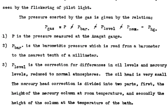
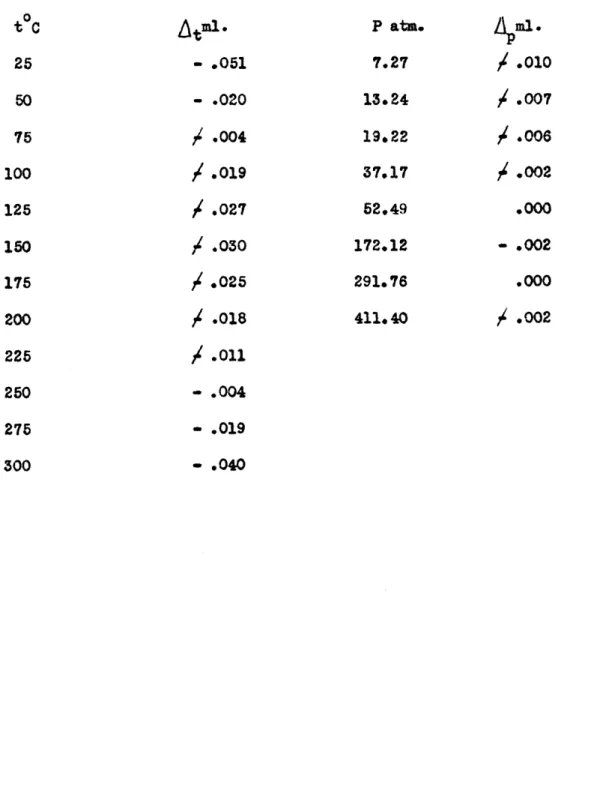
-4-II. Experimental Procedure

The apparatus used to measure the compressibility of gases is

fully described in the literature (31). The method used consists in

confining a weighed amount of gas in an all-steel bomb, by means of mercury. During the course of the measurements the bomb is placed in an oil thermostat where temperature is controlled by means of a phase

shifting thyratron circuit which operates a resistance heater located in the bath. The temperatures range from 150 to 300° C.

Pressures are measured on an Amagat dead weight gauge. The

pressure is transmitted from the confined gas by means of mercury. The pressures range covered in these etperiments was from 30 to 400

atmospheres.

Volumes are measured by means of a mercury injector which, when

calibrated, can be used to add or remove from the bomb known amounts of mercury. By this means, the volumes may be so adjusted that even

densities may be set during the course of the measurements at any given

isothera. The injector is placed in an oil bath, the temperature of

which is regulated at 300 C.

Temperatures are measured by means of a platinim resistance thermometer, and the resistances are measured 6n a Mueller Bridge.

Details of the apparatus and its calibration are given in the Appendices (A, B) as are the corrections which are applied in order to obtain the corrected volumes and pressures.

~I- --

-

(15)

6-III. Compressibility and Equation of State of Ammonia

The ammonia used in this research was obtained from the Matheson Corporation, and had the stated purity of 99.9%. The gas was further

purified by treatment with sodium to remove any traces of water and by

low temperature fractionation as described in Appendix (C).

An attempt was made to determine the vapor pressure of the aiaonia

at a series of temperatures.

However, during the course of our

measure-ments at the

300 isotherm, it was noted that the pressure varied with

the vapor

volume, indicating the presence of a permanent gas.

The first

loading was discarded.

Before the second loading the gas was again

purified in a manner described above and greater precautions were

taken to remove any of the impurities that were present. We still found

that the vapor pressure curve was not flat at the 300

isotherm, indicating

again the presence of some permanent gases.

An estimate was

made as

to the amount of impurity present and it was found to be about 0.02 mole

per cent.

It was concluded that, although some impurity was present,

the amount was negligible for our purposes.

We therefore proceeded to

measure the compressibility of the gaseous ammonia above its critical

point, starting at 1500 and proceeding in steps of 250 to 3000 and at

densities of

1.0, 1.5,

2.0, 2.5,

3.0, 3.5, 4.0, 4.5, 5.0, 6.0, 7.0, 8.0,

9.0, and 10.0 moles per liter. The measured compressibilities are given

in Table I.

It was found in the course of these measurements, that at the

higher temperatures, some of the ammonia had decomposed.

At 3000 this

amounted to between 0.2 to 0.3 per cent, at 2750 to about 0.2 per cent,

at 250

°

to about 0.1 per cent, and below 250

°

the amount of decomposition

(16)

-6-was negligible.

Measurements have _{been made in the past on the compressibility}

of ammonia which overlap part of the region studied-in this investigation.

Thus Beattie and Lawrence (8) report measurements on ammonia

which

cover

the range of from 1500 to 3000 and from 1 to 3 moles per liter in density.

Their measurements, interpolated to our measured densities, are compared

to those reported here in Table II where it is seen that the. average

over-all per cent deviation is 0.292. The experimental error is given

as 0.3 per cent.

J.S. Kasanowsky

(9)

has also reported measurements on the

compressibility of ammonia at temperatures ranging from 2000 to 3000

and at pressures of from 30 to over 1500 atmospheres.

At four different

densities his measurements overlap the region studied in

this

investigation. In Table III his measurements are compared with those

obtained in the present work, where it is found that the average

over-all per cent

deviation

is 0.425%.

He reports his over-all experimental

error as 0.5%.

For the measured densities, pressures, and temperatures given

in Table I, the equation of state constants were calculated using the

method of Beattie and

_{Bridgman (3) and discussed briefly in the Appendix}

(E). It

_{was found that a satisfactory fit could be obtained for ammonia}

for the density range of from 1 to 8 moles per liter inclusive. The

constants obtained are given in Table IV.

The molecular weight used was 17.032 grams and this was obtained from the 1950 reports in the Journal of the American Chemical Society (28)

(17)

on the atomic weights of the

elements.

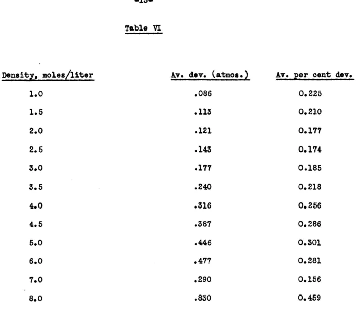
In Table V the observed pressures and the deviation of the observed from the calculated pressures are given. In Table VI the

average deviation of the calculated pressures from the measured

pressures are given, as are the percentage deviations, for each of the isometrios.

(18)

Table I

Compressibility of Gaseous Amonia

Temp. oC. ( Int. )

Density, moles/liter 150 175 200 Pressure, 225 250 standard atmospheres 31.42 44.84 56.88 67.65 77.26 85.80 93.38 100.10 106.04 115.91 123.58 129.56 134.27 33.76 48.55 62.08 74.45 85.74 96.05 105.46 114.06 121.92 135.75 147.47 157.56 166.41 36.05 52.17 67.14 81.03 95.93 105.93 117.08 127.49 137.21 154.86 170.54 184.71 197.74

38.33

55.73

72.08

87.45

101.91

115.53

128.38

140.53

152.06

173.45

193.04

211.33 228.49 40.56 59.26 76.96 93.75 109.72 124.92 139.42 153.27 166.55 191.63 215.10 237.34 258.91 42.80 62.75 81.79 100.01 117.48 134.24 150.36 165.90 180.94 209.65 236.98 263.30 289.04 44.96 66.12 86.45 106.03 124.93 143.19 160.85 178.03 194.93 226.98 285.03 288.57 318.26 1.0 1.5

2.0

2.5 3.0 3.5 4.0 4.5 5.0 6.0 7.0 8.0 9.0 10.0 275 300 138.09 174.39 210.01 245.17 280.03 314.80 348.71 .. -t 'o ... nr?:

(19)

-8-Table II

Comparison of the pressures obtained by Apt and Connolly with those obtained by interpolation from the measurements of Beattie and Lawrence for gaseous ammonia

Temp. oC. (Int.) 150 175 200 225 250 276 300

Density, moles/iter Pressures, standard atmospheres

1.0 Apt. and Connolly 31.42 33.76 36.05 38.33 40.56 42.80 44.96

Beattie and Lawrence 31.47 33.80 36.12 38.41 40.66 42.92 45.11

A. &C. - B. & L. -0.05 -0.04 -0.07 -0,08 -0.10 -0.12 -0.15

1.5 Apt and Connolly 44.84 48.55 52.17 55.73 59.26 62.75 66.12

Beattie and Lawrence 44.92 48.64 52,28 55.89 59.42 62.88 66.35

A. & C. - B. & L. -0.08 -0.09 -0.11 -0.16 -0.16 -0.13 -0.23 a

2.0 Apt and Connolly 56.88 62.08 67.14 72.08 76.96 81.79 86.45

Beattie and Lawrence 56.99 62.24 67.34 72.34 77,23 82.00 86.77

A. & C. - B. & L. -0.11 -0.16 -0.20 -0.26 -0.27 -0.21 -0.32

2.5 Apt and Connolly 67.65 74.45 81.03 87.45 93.75 100,01 106.03

Beattie and Lawrence 67.75 74.64 81.23 87.76 94.11 100.32 106,43

A. & C. - B. & L. -0.10 -0.19 -0.20 -0.31 -0.36 -0.31 -0.40

3,0 Apt and Connolly 77.26 85.74 93.93 101.91 109.72 117.48 124.93

Beattie and Lawrence 77.46 85.92 94.34 102.43 110,29 118.05 125.42

A. & C. - B. & L, -0.20 -0.18 -0.41 -0.52 -0.57 -0.57 -0.49

Total average deviation (atmos.) is .226 Total average per cent deViation is .292

(20)

Table (III)

Comparison of the Pressures Obtained by J.8. Kasarnowaky with those Obtained by Interpolation from the Measurements of Apt and Connolly

for Gaseous Ammonia

Temp. oC. (int.) 200 225 250 275 300

Density, mole/liter Pressures, standard atmospheres

3.216 Apt and Connolly 99.92 107.88 116.36 124.79 132.87

J.S. Kasarnowsky 100.2 108.6 117.0 126.4 133.8

A. & C. - J.8.K. .0.98 -0.72 -0.64 -0.61 -0.93

5.000 Apt and Connolly 137.21 152.06 166.55 180.94 194.73 o

J.S. Kasarnowsky 138.3 152.5 166.7 181.0 195.2

A. & C. - J.S.Ko -1.09

-S0.W4

-0.15 0.06 *0.47

6.667 Apt and Connolly 165.54 186.64 207.40 227.98 247.79

J.o. Kasarnowsky 166.0 186.8 207.5 228.2 249.0

A. & Co. J.S.K. -0.46 -0.16 -0.10 -0.22 -1.21

10.000 Apt and Connolly 210.01 245.17 280.03 314.80 348.71

JS. Kasarnowsky 208.0 243.3 278.6 513.9 549.2

A. & C. - J..K. /2.01 1.87 /1.45 /'0.90 -0.49

Total average deviation (atmos.) is 0.747 Total average per cent deviation is 0.425

(21)

Table (IV)

Values of Canstants for the Beattie-Bridgman Equation of State for Gaseous Ammonia

P RT (1

-.

)/V2 V/B A/V2

A

A(1

-

a/v)

B * Bo(1 - b/v)

Units; normal atmospheres, liter per mole, oK (ToK . toC

/

273.13)

R a 0.08206

A

0

X 5.936

a a 0.05244

b

a

0.05281

o

10010o

4

B

_o

I 0.08970

(22)

Gaseous Ammonia

Temp.

oC.

(int.)

Density, moles/liter.

150 175

200

225

250

275

Pressures, standard atmospheres 1.0 obsd. obsd-calo. 1.5 obsd. obed-cale. 2.0 obed. obsd-oalo. 2.5 obed. obed-calo. 3.0 obed. obsd-oalo. 3.5 obed. obed-oalo. 4.0 obed. obed-calo. 4.5 obed. obsd-oalo. 5.0 obad. obsdroalo. 6.0 obsd. obsd-oalo. 7.0 obsd. obsd-oalo. 8.0 obsd. obad-ealo.

31.42

33.76 -0.13

,0.07

44.84

48.55 -0.23

-0.11

56.88

62.08

-0.32 -0.12

67.65

74.45

-0.39 -0.09

77.26

85.74

-0.42 -0.04 85.80 96.05 -0.41 /0.06

93.38

105.46

-0.35 /0.18

100.10

114.06

-0.26 /0.32 106.04 121.92 -0.14

/0.

44

116.91

135.75 /0.o01

/0.56

123.58

147.47

-0.23 /0.21

36.05 -0.05

52.17 -0.05

67.14 -0.01

81.03 -0.05

93.93 /0.14

105.93 /0.28

117.08

/00.41

127.49 /0.56

137.21

/0.69

154.86 /0.77

170. 54

/0.36

38.35

-0.04

55.73 -0.04

72.08 -0.00

87.45 -0.07

101.91 /0.18

115.568 /0.31

128.38 /0.44

140.53 /0.58

152.06 /0.

70

173.45

/0.76

193.04

/0.37 40.56 42.80 44. 96

-0.06

59.26 -0.05 76.96 -0.03 93.75 -0.02

109.72 /0.10

124.92 /0.20 139.42 /0.32

153.27

/0.43 166.55 , .52 191.63 /0.59

215.10 /0.27

0.08

62.75 -0.08

81.79 -0.08

100.01 -0.05

117.48 /0.02

134.24

/0.09

150.36 /0.18

165.90 /0.28

180.94 /0.38

209.65 / 0.45 236.98 /0.28

-0.17

66.12 -0.23 86.45 -0. 29 106.03 -0.33 124.93 -0.34 143.19 -0.33 160.85 -0. 33

178.03 -0,28

194.93 -0.25

226.98 -0.20 285.03

-0.31

129.56

157.56

184.71

211.33

237.34

263.30

288.37 -1.32

-1.03

0.90 -0.74

-0.74

-0.41

-0.67

300

_L .... ressresstanard tmoshere -12-Table (V)

Comparison of the Pressures Calculated from the Equation

(23)

Table

VI

Density. moles/liter

1.0

1.5

2.0

2.5

3.0

3.5

4.0

4.5

5.0

6.0

7.0

8.0 Av. dev. (atmos.)

.086 .113 .121 .143 .177 .240

.316

.387 .446 .477 .290

.830

Av.

per cent dev.

0.225

0.210

0.177

0.174

0.185

0.218

0.256

0.286

0.301

0.281

0.156

0.459 Total average deviation

(

atmos.

)

from

1 to 8

moles

per liter

a .302

(24)

-14-IV. Virial Coefficients for Ammonia

A. Second Virial Coefficients from the Stockmayer Potential

Instead of using a closed form for the equation of state, such

as that used by Beattie and Bridgman, Kamerlingh-Onnes (46) has shown that compressibility measurements may be correlated by using an equation of state of the type:

PV

RT

/

B/V /

C/V

2

_/

_...

₍₁₎

Here B is known as the second virial coefficient and C is the third virial coefficient. Both B and C and the higher terms are functions of

the temperature.

In the present work, for calculating these virial coefficients, use is made of the function By which is defined as:

8,

:

V(V - RT)

B/

C/V

/

... (2)

In equation (2)

B

and

C are the second and third virial coefficients

respectively. To determine B and C it was assumed that Bv may be expressed in terms of the density in the following way:

Bv : B /C/V / D/V (3)

The constants B, C and D are determined by the method of least squares. It is obvious that the constants B and C are the second and third virial

ooefficients appearing _in equation (1) under the assumption that the term

3

in 1/V takes care of the higher terms. In Table VII the values of B_vare given and the deviations of these values from those calculated by the

method of least squares are listed underneath. In Table VIII values for RT

(25)

The values for B, C, and D of equation (3) are given, for the seven temperatures from 1500 to 3000 in Table IX.

It has been shown, for example, by the application of the virial

theorem of Clausius that B may be expressed by (13):

B

:

1/2

N (1

e.xp

_{(- (q)/kT)}

₎

₍₄₎

where the integral is taken over volume, N is Avogadro's number and W(q)

is the mutual potential energy of a pair of molecules as a function of

their space co-ordinates q, and dv is the

volume

element in phase space.

Stookmayer (14) used for the complete potential energy between

a pair of polar molecules the equations

-6

2 -S

w(q)

A~

-

or

-

pr g

(5)

where N and o are constants, r is the intermolecular distance, p is the dipole moment, which for ammonia is given (15-19) as 1.46d, and g is the

geometrical factor of the form:

g . 2 cos ,, cos.. - sin.E), sine os, (6)

This potential may also be

written

in the

form:s

where Rij

:

rij/r, tl

:

1/8 (p2/ (ro0)3), and kT/. and

ro are the energy and the distance characteristic of non polar part, if p

is equal to zero, then ro is the distance at which w(q) : 0, and - E is

the minimumn value of W(q). The angles given in equation (6) E, , O_

and

4 ,

specify the inclinations of the two dipole axes to the

intermolecular axis, the azimuthal angle between them.

Equation (4) may be rewritten in the form:

B(T) : N/4 ( 1 - exp(-q)/kT ) r2 dr dA# whe re

Id

:

sin e,

sin

e,

d,d

OS

:c

81 (8)

(26)

and solving the integral using the Stookmayer potential given in equation (5) above, the solution obtained is:

S2k 3 B(T) z bo(4/)

T()

1/4 2/n k (2n-2k2/4) t

wh re;(

((9)

G

_k

: 1/(2k

1)

(

3 ( s2J/

1)

b 3 o : 2/3 (T Nro) tl 1-8 (p2/E'(ro)3

(o)

Rowlinson (20, 21) defines the function Bp2 (T) such that

B (T) :b

_o

Bp2 (T)

(10)

and tables of this function as well as tables of the function 7'/t Bp (T) are given by him in the references listed above. He also sets out a method

of curve fitting for the Stockmayer potential. This method was used in

the present calculations.

Both the calculated and observed second virial coefficients are given

in Table X. In the first column are the values obtained in the present

work, in the second column are the values obtained by Lawrence (22) from

his measurements on the compressibility of amonia, by the extrapolation of

the Bv values given by equation (2). That is,

in the B

_v

versus 1/V plots

he made, he extrapolated the curves so obtained to I/V = 0. The intercepts

are the second virial coefficients for the various temperatures.

The

agreement between these two sets of measured values of B(T) is quite good.

In the third

column

of Table X are found the theoretical values of B(T).

The agreement between the observed second virial coefficients and those

calculated using the Stookmayer potential is very good.

(27)

The parameters used to fit the second virial coefficients to

Stookmayer's potential are given in Table XI. These parameters were used to construct the series of potential energy curves, 1, 2, and 3 of

Figure 1. Curve number 1 is the one obtained when P, the dipole moment,

is equal to zero. We would then have just the Lennard-Jones potential. In the case where the dipoles are oriented so that they exert a maximum of

attraction on one another, the depth of the minimum is greatly increased. This is seen in curve 2 where the depth of the minimum is nearly 6 times that of curve 1. On the other extreme, when the dipoles are so oriented that they exert a maximum of repulsion on one another, then the potential energy curve obtained is one of pure repulsion. This may be seen in curve 3.

(28)

F

-18-w

Table (VII)

Values of

B(V,T)

for

Ammonia,

B(VT) a V(pV

-

RT) (observed)

B(V,T) * B(T)

/

C(T)/V / D(T)/ 3

(oalculated, see Table (Ii) )

Temp.

C

(int.)

0 Temp.

K

RT, liter-atmos./mole

Density, mole/liter

150

423.183 37. 7241

175

448.198 36.7767

200

473.214 38. 8293

B(V,T),

225

250

498.231 523.248 40.8821 42.9348 liters2 -atmos/mole2 275 548.264 44.9875 1.0 obsd.

obsd.-cale.

1.5 obsd,

obsd.

-cale.

2.0 obad.

obsd, -cale.

2.5 obsd.

obsd.*cale.

3.0 obsdo

obsd.

-cale.

3.5 obsd.

obsd. -calo.

4.0 obsd.

**obs d.* ale o**

4.5 obed.

obed.

-calo.

5.0 obad.

obs d.

-cale.

6.0 obed.

obsd.o-oale.

7.0 obsd.

obsd. -alc

8.0 obesd

obsd.e

**cal*e**

300

573.278 47.0400

-. 30410

-0.00515

; .22053

00092

-3.14205

/0.00239

,3.06564

/0.

00244

"2.99027

/0.00228

**"2*01709**

/0.00090

-2.84478

-0.00020

-2.77327

0.00080

-2.70322

-0.00139

-2.56763

-0.00200

-2.43854

-0.00128

-2.31614

/0.00191

-. 01670

-0.00686

-1.94000

.00033

"2.86835

/0.00295

-2.79868

/0.00423

2.75223

/0.ooo08

-2.66680

/0.00187

-2.60292

/0.00022

2.564000

0.00111

-2.47854

-0.00247

-2.35862

-0.00326

-2.24423

0.00192

-2.13521

/0.00296

*2.77930

0.01361

-2.69953

/0.00159

-2.62965

/0.00742

-2.56692

/0.00680

-2.50643

/W,00480

-2.44674

/0.00305

-2.38982

-0.00025

-2.33293

-0.00219 -2.27746

-0.00398

-2.16988

-0.00554

-2.06663 -0.00507 -1.96756 /0.00497

-2.55210

-0.00866

.2.48567

-0.00180

-2.

42105

/0.00412

*2.36084

/0.00607

-2.30403

/0.00541

w2.024957

/0.00335

-2.19678

/0.00073

-2.14516

-0.00179

2.09402

-0.00337

-1.99563

.0.00550

**-*1.90071**

-0.00350

**"*1.80824**

/0.00492

-2.37480

-0.02328

*2.28540 /0.00895 -*2.22740 /0.01032 -2.17392 /0.00788 -2,.12050 /000628 -2.06954 /0.003528 2.01995 /0.0017 -1.97218 "0.00334 -1.92496 -0.00579

-1.

83275

-0.00738

-1.

74374

-0.00560

-1.65841

/0.00649

**-*2.18750**

-0.02317

-2.18750

/0.00709

.2.04625

/0.00973

-1.99340

/0.00939

1.94250

/0.00801

**-*1.89520**

/0.00410

-1.

8493 8

-0.00005

-1.

80462

-0.00377

-1.75990

-0,00594

-1.67430

-0.00853

-'1, 5046

-0.00424

-1.50938

/0.00736

-2.08000

-0.05823

,.97333

.00961

-1.90750

/0.01741

-1.86120

/0.01674

-1.79890

/0.01340

-1.75103

/0.00721

-1.70688

-0.00085

-1.66173

-0.00579

**-*1.61880**

-0.01056

-1.

53500

-0.01398

-1.

45409

-0.00758

-1.37422

/0.01260

_ _I _ __ __ C___~ _ _ ___ _ ~~

(29)

T

O

C

_{( Int. )}

150

175

200

225

250

275

500 TC

(th.)

423.183 448.198 473,214 498.231 523.248 548.264 573.278 RT 34. 7241 36.7767 38.8293

40.8821

42.9348 44. 9875 47,0400

The thermodynamio centigrade temperatures were calculated from the equation reocommended by the 8th General Conference of the International Committee on Weights and Measures.

t(th) : t(int)

j

t/100(t/100-1) (.04217 - .00007481t)

T

t(th) 4 273.16.

Table (VIII)

(30)

~I~

Temp.

oC (Int.)

150 175 200 225 250 275 300

B(T)

liter

2

-atmos.

per

1mole

2 -3.4547566 -3.1496547 -2.8957059 -2.6629700

-2.4667501

-2.2741257

-2.160735

CT)

liter -atmos.

per moleS

0.15603054

0.14002648

0.13024572

0.11974363

0.11546634

0.11003279

0.11932069

D(T)

x104

liter5-atmose per mole5 -2.1783784 -2.1234934 -2.3200428 -2.1121777 -2.3804932 -2.3999670 -3.5284451

420-Table (IX)

Second and Third Virial Coeffioients of Ammonia

pV a

RT

/

B(T)/V

_{/ C(T)/V}

2

_/

D(T)/V

4

Ill I

- --- --- -

(31)

---21-0

Table (X)

Comparison of the

Observed

Seoond Virial Coefficients

with

those Calculated Using

Stockmayer's

Potential for Polar

Gases,

for Gaseous Ammonia.

To (therm.)

423.183 448.198 473.214 498.231 523.248 548.264 573.278

B(T),

oo/mole

present investigation

99.5

85.6 74. 6

65.1

57.5

50.6

45.9 B(T), oc/mole

Lawrence

99.7

85.7

74.7

65.4

57.5

50.7

44.5 B(T), co/mole

calculated

99.3

86.4

74.6

65.4

57.5

50.6

45.9

The average deviation is *0.2 co/mole

(32)

---

-22-Table XI

The Parameters Used for the Fitting of the Stookmayer Potential

Are:

t

_-

_1.2

8/k

=

284.6 b

:

-

_{20.17 cm}

3

_/mole

-8

ro

-

2.5190 x10

cm.

E'

-

3.9289 xl1014 ergs/degree

p

:

1.46 Debeye

In the curve fit it was necessary to assume at one stage that

the

values B(T) could be represented by the equation:

a

B(T)

:

AT

and a plot is made of log B(T) against log.T, and the slope of the

best straight line is then given by s. This quantity is necessary

in the curve fitting process so it is given

here:

(33)

C(T), the third virial coefficient, provides a more severe

test of molecular models than the second virial coefficient B(T), in

that it is more sensitive to the shape of the potential. This will be

seen in the comparison that is made between the agreement of the

observed vat ues of the second virial coefficients and those obtained from the Stockmayer or Lennard-Jones potential with the agreement obtained between the observed values of the third virial coefficients

and those calculated using the Stockmayer or Lennard-Jones potential. The third virial coefficient is given by:

C(T)

-

N/

ff

f

1

2fl3f2

3

dr dr

2

(11)

where;

fij

exp(-W(q)ij/

₁

₎

where W(q)ij is the energy of interaction of molecule i and j and

depends on their distance apart and their

relative

orientation and is

given by equation

(5).

Hirschfelder, Bird, Spotz, and Curtiss (23) have calculated the third virial coefficients for gases obeying the Lennard-Jones

potential,

W(q)/kT :

(4/')

R

-12

-

Rij'6

(12)

using high speed calculators. Rowlinson (23) has carried out the

calculations

for the

polar part so that combining the work of Hirsohfelder,

Bird, Spots,

and

Curtiss with his own, he constructed a table of values

for the third virial coefficients for the Stockmayer potential in terms of the parameters tl and

T

, which parameters are obtained on fitting the second virial coefficient.

(34)

I

In Table XII are given the third virial coefficients as determined from experiment by the method of least squares, and the third virial coefficient as determined by the calculations of Rowlinson et al.

The agreement between the observed and the calculated third

virial coefficients may be considered fair. One must take into account

firstly that the accuracy of the calculated values is not given in Rowlinson's paper. Secondly, the experimental values of the third virial coefficient were obtained from a three turn polynomial, while generally good enough to give B(T), it does not yield the best values of C(T). If one looks, for example, at the values of B(T) and C(T) obtained from experimental measurements by Hirschfelder et al., one

sees that with more terms in the polynomial the second virial coefficient changes very little whereas there are sizable changes in the values

of C(T) (23).

(35)

-24-Table XII

Comparison of the Measured Third

Virial

Coefficients

With

Those Calculated Using

Stockmayer's

Potential

for

Polar

Gases, for

Gaseous

Ammonia.

0 T (therm.) C(T) co2/mole2 observed

423.183

448.198

473,214 498.231

523.248

548.264

573.278 4493.4 3807.5 3354. 3 2929.0 2689.3 2445.9 2556.6 C(T) c 2/mole2 calculated 3300 2970 2630 2300 2020 1800

1610

_ ___~

(36)

28.-C. Second Virial Coefficients from the Lennard-Jones Potential.

For comparison with the Stookmayer potential,

caloulations

of

the second virial coefficient

of

ammonia were made for the

Lennard-Jones potential (25) which

may

be written as:

W(q)

r

r-

1 2

s

-6

t4q)

-

(

r)

- I u > /iiLi ergs

6 -

>/f

°m.

2 N

6."/3

The method used for obtaining the parameters of the potential

was the one given by Stockmayer and Beattie (26) who found that in the

range of (/T of 0.2 to 1.0, B(T) could be represented by the equation:

B(T)

_:

(1.064

-

3.602 e/T

)

(14)

From a plot of BT

/ 4

_{against 1/T}

_and

_{#may be determined since}

**-3*.60205**

1

4 is the slope and 1.064

is the intercept on the

BT

1/ 4

axis at 1/T

-

0 of the best straight line through the experimental

points.

(37)

O -I -2 -3 -4 -5 -6 1.0 1.2 1.4 1.6 1.8 2.0

r/

Figure 1

(38)

-27-found that

-369.003

:

-3.602

(3

5/4

and

428.8

1.064 1/4

then S-: 254.199

:,

"

403.0

and then the equation becomes

B(T)

:

403.0 /T (1.064

915.621/T

)

(15)

which was used to calculate the second virial coefficients.

The results are shown in Table XII and these are compared with the observed second virial coefficients whence it is found that the average over-all deviation is 70.84 co/mole.

In Table

XII

the parameters of the

Lennard-Jones

potential

are given. From these parameters, curve 4 of figure 1 was plotted. Here it may be noticed that, although the value of E obtained using Stockmayer's potential has nearly the same value as that obtained using the

Lennard-Jones, ro, the value of r when E(r) O0, is nearly twice as large for the

Lennard-Jones potential.

The second virial coefficient is not nearly so sensitive to the

form of the potential energy function used as is the third. Thus we find

that the calculated values of the second virial coefficient using the

Lennard-Jones potential gives almost as good agreement with observed values as

does Stockmayer's. However, great differences are encountered on examining

(39)

Table XIII

Comparison of the Observed Second Virial of Ammonia With Those Calculated Using the Lennard-Jones

Potential

T (therm.) B(T) co/mole B(T) co/mole

Observed Caloulated

423.183

99.5

97.7

448.198 85.6 85.7 475.214 74.6 75.3 498.231 65.1 66.0 523.248 57.5 57.8 548. 264 50.6 50.5 573.278 45.9 43.9

(40)

-29-Table XIV

Lennard-Jones Parameters

:

350.9203 x10-

1 6

ergs

/I

A:

-58 8.9860 xlO -102 5.7526 x10

ergs

cm

6

ergs

cm

12 om o S: 4.3091 A

r

21/6

o 2 6

23 N

6.023 xlO

k

:

1.3805 xlO0

16 0 4.8368 A erg deg.

were obtained from Birge (45).

'Where

(41)

D. Third Virial Coefficient from the Lennard-Jones Potential. Using the parameters obtained by fitting the Lennard-Jones potential for the second virial coefficients and the tables set up

by Hirschfelder, Bird, Spots, and Curtiss (23), the third virial coefficients were calculated. These caloulated values are given in Table XV.

The agreement between the observed and the calculated values of the third virial coefficients, as is shown in Table XV, is quite

poor. One may say, therefore, on comparing the agreement found here

with that found using the Stookmayer potential, that this latter

potential

is the more realistio one in this

case.

(42)

To (ther.)

C(T)

co

2

/mole

2

Observed

425.183 448.198 475.214 498,231 523.248 548.264 573.278 4,500 3,800 5,400 2,900 2,700 2,400 2,500

C(T)

o2/mole

2 Calculated

10,250

9,800

9,400 9,000 8,700 8,500 8,200

_

__

_ _

__

______

-31-.

Table XV

Comparison of the Observed and the Calculated Third Virial Coefficients for Gaseous Ammonia Using the

(43)

V. Compressibility and Equation of State for the Gas Mixture

Ammonia-Methane

A. Introduction

The methane used in this investigation was obtained from the

Phillips Petroleum Company and had the stated purity of

99.5%.

The

gas was further purified by low temperature fraotionation as

described

in Appendix (C). The ammonia was obtained from the Matheson Corporation

and purified in a manner as described above and in Appendix (C).

The mixture reported on here consisted of 29.849 mole per cent

ammonia and 70.451 mole per cent methane. The measured compressibility

of

this mixture is given in Table

XVI. Here, as in the case of the measurements on the pure ammonia,

decomposition was found to occur at the higher temperatures amounting

to 0.17%o at the highest temperature, i.e., at 3000, and becoming

progressively less at the lower temperatures, being negligible at

2500 and below.

B. Non-Polar Combination

The equation of state constants for the mixture, Aomr am

Bom, bm and am were obtained in two different ways. In the first method,

using what we termed to be the non-polar combining rules, Aol2 and C12

were obtained by a square-root method, Bol

₁₂

from a Lorentz combination,

and a

12

and b12 from a linear combination of the equation of state

constants of the pure components, methane and ammonia.

Thus#

om

(iiA/1/2

2

(44)

2 /, 1/3B 13 2 Bo2

Sxi, Boi / 1/4x x₂ (Bo1 /Bo 2

)

/ x 2 B 2

1/

2 Om

:

(Xii/2)

am

-

xla

/

x

₂

a

₂

b

:

bi

x

₂

b

2

so that the equation of state for

n

i

moles of gas may be written as;

P 'nRT 4

-Vi

2 V

3 4 V V4

(17)

V V

"0 RTBm

-

Aom

-

RC

_m T2

:

RTBomb

/Aom

RBomCm

IM _-0

- RB b

c

- omn mm

2

T

General physical considerations indicate the square root

combination for the attmrative constant

A

o

, which

corresponds to the

a

in Vander Waals equation, and the

Lorentz

for the repulsive

constant

Bo, which

corresponds to b in the Van der Waals

equation,

this

latter

(45)

5'3-type of combination corresponding to the averaging of the radii of the

molecules.

In addition, in a study on

the compressibility of gaseous mixtures

of methane and normal butane, Beattie, Stockmayer, and Ingersoll (27)

found that the above combination rules could be used to reproduce the

compressibilities

of the mixtures almost as well

as

the equation of

state represented the properties of the pure gases.

Before these rules could be applied to the mixture reported here,

the equation of state constants for the pure methane had to be corrected

for the

revised atomic weights of the element.

In the 1950 report of

the Committee on Atomic Weights

of

the American Chemical Society (28),

the

atomic

weight of carbon is given as 12.010 grams and that of hydrogen

as 1.008 grams. This gives for the molecular weight of methane 16.042

grams. The equation of state constants for methane calculated by Beattie

and Bridgman were based on a molecular weight of 16.0308 grams. This

meant that all of the constants had to be

recalculated on the basis of

the new molecular

weights.

Dimensional analysis

shows

that

R, a, b, Bo,

and

c

may be corrected by multiplying these constants by the ratio of the

molecular weights and that Ao, which is given in terms of liters

2

-atmos.

2 per mole had to be corrected by multiplication by the square of the

ratio of the molecular weights. This was done by

Stockmayer

(11) and the

corrected constants for methane are given in Table

XV. In Table

XVII

there may be found the

measured compressibilities

of

the gas mixture

and

the deviation

of

the observed pressures from those

(46)

-35-equation (16) above,

are

given in Table

XVIII. Here it

is

found that

the average over-all percent deviation is

1.07. The equation of state constants for the mixture using the

"non-polar" oombination rules are given in Table XIX.

(47)

Table (XVI)

Compressibility of the Gaseous Mixture Methane-Ammonia Consisting of 29.849 Mole Per Cent Ammonia and

70.151 Mole Per Cent Methane

C (int.) moles/liter 150 Temp. o Density,, 1.0

1.5

2.0

2.5

5.0 3.5 4.0 4.5 5,0 6.0 7.0 8.0 9.0 10.0 175 36.06 53.69 71.12 88.39 105.56 122.66 139.75 156.90 174.12 209.13 245o21 282.99 323.02 365.85 200 Pressure,

38.22

57.08

75.70

94.28

112.81

131.34

149.94

168.64

187.50

225.95 265.83 307.72

352.16

399.89 226 250

275

300 standard atmosphere 40.37 42.51 44.68 46.83 60.35 80.24 100.10 119.98 139.92 159.97 180.22 200.67 242.58 286.15 332.05 380.91 63566 84.78 105.91 127.13 148.48 170.02 191.81 213.87 259.18 306.55 356.53

67.02

89.37

111.80

134.39

157.18

180.18

203.53

227.25

276.02

327.15

381.17 70335

93.91

117.63

141.61

165.83

190.33

215.23

240.55

292.84

347.71

405.87

33.89 50.34 66.52 82.49 98.27 113.92 129. 51 145.06 160.64 192.11 224.37 257.94 293.30 331.17 --- ~- -- --~-- -- ~ --- ~-- - - -- ~--~- --- --- ----

(48)

--Table (xVII)

Comparison of the Pressures Caloulated from the "Non-Polar"

Combining Rules with the Observed Pressures for the Gaseous Mixture 29.849 Mole Per Cent Abmonia, 70.151 Mole Per Cent Methane

Temp.

oC (int.)

Density, mole/liter

150

175

200

225

250

275 Pressures, standard atmospheres

1.0 obsd. obed. *-oalo. 1.5 obed. obed ,caleo. 2.0 obud. obsad.cal. 2.5 obad. obad. -calo 3.0 obsd. obsd.*calo. 3.5 obed. obsd. "calo 4.0 obed. obed.-calo. 4.5 obsd. obsd. -calo. 5.0 obad. obad.-calo. 6.0 obad. obsd.-cale. 7.0 obed. obad.-calo. 8.0 obsd. obsd. calo.

33.89 /0.14

50.34 /0.37

66.52 /0.69

82.49 /1.12

98.27 +1.62

113.92 /2.19

129.51 /.85

145.06 /8.57

160.64 /4.35

192.11 /6.13

224.37

6.21

257.94

40.67

36.06 '0.10

53.69 /0.30

71.12 /0.59

88.39 /0.95

105.56 +1.40

122.66 . 90o

139.75 /.47

156.90 /A.11

174.12 /2.79

209.13 /6.39

245.21 /7.25

282.99 /9.58

38.22 /0.06

57.03 /0.23

76,70

,0.47

94.28 /0.79

112.8 +1. 1b

131.34 4. 59

149.94 /,.08

168.64 /2.62

187. 50

/6.21

225.95 /4.56

265.83 /6.24

307.72 /8.38

40.37

A.02

60.35 0, 14

80.24 /0.33

100.10 /0

.57

119.98 +0.87

139. 92

/1.20

159.97 /1.58

180.22 /2.02

200.67 /2.48

242.58 /2.64

286.15 /4.06

332.05 /6.97

42.51

44.68

46.83

0.04

63.66

84.78 /0.19

105691

/0.36ss

127.13 +0.57

148.48 /0.82

170.02 /1.12

191.81

41.47

213.87 /1.83

259.18 /2.75

306.55 /4.06

356, 53

/5. 85

a0.06

67.02

0.01

89.37 ,.

10

111.00 p,. 22

134.39 +0.39

157.18 f0.60

180.18 /0.80

203.53 A1.08

227.25

1.40

276.02 P0.18

327.15

4.35

381.17

6.02z

-0.11

70.33 **#*0.07**

95.91 -0.03

117.6 /0.04

141,61

+0*18

165.83 ;/0.34

190.33 /0.49

215,23

/0.69

240.55 /0.92

292.84 /.63

347.71 /2.68

405.87 /4.34

300

- - ~--

(49)

-Deviations "non-polar" Combination

Density,

moles/liter

1.0 1.5

2.0

2.5 3.0 3.5 4.0 4.5 5.0 6.0 7.0 8.0

Total

average

Av. dev. .076 .167 .343 .577 .gg4 1.234 1.627 2.080 2.569

3.754

5.264 7.529

deviation (atmos.)

per cent deviation

from

1 to

from 1 to

(atmos.)

Av. per cent dev.

.194

.303

.467

.629

. 799

.954

1.100

1.248

1.384

1.671

1.979 2.339

8 moles

per liter

:

8 moles per liter r

2.153

1.089

(50)

15C1- ---- - -L

1-Methane

0.082117

2.2801

0.05591

-0.01588

0.01856 12.84 x 10 4 Ammonia

0.08206

5.936 0.08970 0.05281

0.05244

4

100 x 10 Mixture

0.08210

3.19165

0.065441

0.004623

0.028673

50.2348 x 104

-39-Table XIIX

Equation of State Constants Obtained by Using the "Non-Polar" Combining Rules on the Pure Gases,