HAL Id: tel-01184241
https://tel.archives-ouvertes.fr/tel-01184241
Submitted on 24 Aug 2015HAL is a multi-disciplinary open access archive for the deposit and dissemination of sci-entific research documents, whether they are pub-lished or not. The documents may come from teaching and research institutions in France or abroad, or from public or private research centers.
L’archive ouverte pluridisciplinaire HAL, est destinée au dépôt et à la diffusion de documents scientifiques de niveau recherche, publiés ou non, émanant des établissements d’enseignement et de recherche français ou étrangers, des laboratoires publics ou privés.
Computational mechanistic photochemistry: The central
role of conical intersections
Martial Boggio-Pasqua
To cite this version:
Martial Boggio-Pasqua. Computational mechanistic photochemistry: The central role of conical in-tersections. Theoretical and/or physical chemistry. Université Toulouse III, 2015. �tel-01184241�
Manuscrit
en vue de la soutenance de
l’Habilitation à Diriger les Recherches
par
Martial BOGGIO-PASQUA
Computational mechanistic photochemistry:
The central role of conical intersections
Soutenue le 22 Juillet 2015
JURY
Pr. Maurizio PERSICO
Professeur, Université de Pise
Rapporteur
Pr. Nicolas FERRÉ
Professeur, Université d’Aix-Marseille
Rapporteur
Dr. Daniel BORGIS
Directeur de recherche, ENS Paris
Rapporteur
Pr. Isabelle DEMACHY
Professeur, Université Paris Sud
Examinateur
Dr. Thomas GUSTAVSSON
Directeur de recherche, CEA-Saclay
Examinateur
Pr. Fabienne ALARY
Professeur, Université Toulouse III
Présidente
Ecole doctorale : Sciences de la Matière
Foreword
1. Introduction
p. 7
1.1. Computational mechanistic photochemistry
1.2. Role of conical intersections
2. Conical intersections and associated crossing seams
p. 10
2.1. Introduction to the theoretical concept of conical intersections
2.2. Topological features
2.3. The important coordinates in photochemistry
3. Mechanistic photochemistry: theoretical aspects
p. 15
3.1. Determination of potential energy surfaces and reaction pathways
3.1.1. Electronic structure methods
3.1.2. Photochemical reaction path
3.2. Excited-state molecular dynamics
4. Applications: from organic photochemistry to photobiochemistry and inorganic
photochemistry
p. 24
4.1. Organic photochemistry
4.1.1. Photostability of polycyclic aromatic hydrocarbons
4.1.2. Photochromic systems
4.1.3. Intramolecular charge transfer
4.2. Photobiochemistry
4.2.1. Photostability and photodamage in DNA
4.2.2. Photoisomerizations in proteins
4.3. Inorganic photochemistry
4.3.1. Photophysical properties of ruthenium complexes
4.3.2. Photochromic ruthenium complexes
5. Perspectives
p. 57
5.1. Electronic energy transfer
5.2. Photoswitchable systems
5.2.1. Organic photoswitches
5.2.2. Reversibly switchable fluorescent proteins
5.2.3. Inorganic photochromes
5.2.4. Hybrid photochromes
6. Conclusion
p. 63
7. References
p. 64
Foreword
This manuscript is written as an introduction to the field of computational photochemistry. It is not intended to be a textbook, as more emphasis has been made on illustrations rather than on methodologies and technical guidelines. In this way, I hope that it will be accessible to a large audience, from undergraduate students to more experienced scientists who would be interested in learning about this fascinating and relatively young field of research.
This manuscript would have never appeared without many of the people I had the chance to study or work with along these last twenty years or so. First, I would like to thank Prof. Jean-Claude Rayez who taught me quantum chemistry and transmitted his passion to me. I am indebted to Prof. Mike Robb and Dr. Mike Bearpark for all the knowledge they have imparted to me on computational photochemistry and for their support during my scientific career as a post-doctoral researcher. A large part of this manuscript is devoted to the work we have done together. My collaborator, Dr. Gerrit Groenhof, also played a critical role in some of the most successful stories I am presenting in this report. I would also like to thank Prof. Fabienne Alary and Dr. Jean-Louis Heully for giving me the opportunity to work in their team, for sharing their passion of theoretical chemistry with me and for their support during the writing of this manuscript.
Finally, I would like to dedicate this manuscript to my wife, Marjorie. Her support is a great source of motivation for me, and our two children, Lina (4 years old) and Timéo (2 years old) are a source of joy.
1. Introduction
In the past three decades or so, computational photochemistry has gained considerable credit as a tool to investigate photochemical reaction mechanisms in organic, inorganic and even biological chromophores.1 This reputation has been gained thanks to the concomitant growing of computational power and theoretical developments in the field of quantum chemistry. These advances allow peering beyond the traditional interpretations of photochemistry focused on vertical excitations at the Franck– Condon geometry. The exploration of other regions of the complex multidimensional potential energy surfaces is becoming routine, and the synergy between accurate and global static calculations and either quantum or semiclassical nonadiabatic molecular dynamics simulations has allowed major breakthroughs in the understanding of photochemical and photophysical processes. Nowadays, computational investigations of photochemical processes such as photoisomerization, photoinduced electron transfer, photosensitization and photodissociation have become a standard practice.
While standard state-of-the-art ab initio quantum chemical methods are already capable of providing a complete description of what happens at the molecular level during bond-breaking and bond-forming processes in thermal reactions, the task is much more challenging when contemplating photochemical reactions. The main reasons are as follows: i) the description of electronic excited states can become very difficult because of their usual multiconfigurational character, ii) the reaction path cannot be described by a single potential energy surface, but rather two branches at least are required: one located on an excited state (reactant side) and the other located on the ground-state potential energy surface (product side), and iii) the Born-Oppenheimer approximation breaks down in the ‘funnel’ region where the excited-state reactant or intermediate is delivered to the ground state. The main difficulty associated with computations of photochemical processes lies in the correct description and practical computation of this ‘funnel’ region. Computational tools have been developed and strategies discovered to explore electronically excited-state reaction paths involving so-called conical intersections, which act as funnels for efficient radiationless electronic transitions. The goal of such computational approaches in the study of photochemical mechanisms is the complete description of what happens at the molecular level from photonic energy absorption to product formation.
In this manuscript, I will review my own contributions in this fascinating field of research. I will start by giving a short introduction on what is called computational mechanistic photochemistry and the central role played by conical intersections. Then I will review the basic concepts and computational strategy, which permit such investigations. Next I will give some illustrations based on the most interesting systems I had the chance to study. These include the study of organic and inorganic photochromic systems, the photoisomerization of a protein, the photostability of polycyclic aromatic hydrocarbons, photoinduced intramolecular charge transfer in donor-acceptor systems, and photoinduced proton-coupled electron transfer in biological systems. Finally, I will present some perspectives of future work.
1.1. Computational mechanistic photochemistry
The terminology computational mechanistic photochemistry is used in the present manuscript to designate theoretical studies aimed at understanding excited-state mechanisms involved in photochemical processes. The term photochemistry (or photochemical processes) is used here in the
broadest sense, i.e. it also includes photophysical processes such as nonradiative decay back to the original ground state (photostability) and radiative emission (photoluminescence). To understand the fate of a molecular system after photoexcitation, it is not only necessary to understand the excited-state properties of the molecule but also to determine how the system will evolve chemically in terms of bond making and bond breaking in these excited states. Thus, it is crucial to understand the reaction pathway describing the passage from the ground-state reactants to the final photoproducts evolving along the potential energy surfaces (PESs) of the photochemically relevant electronic states. This reaction path is called photochemical reaction path or photochemical pathway. As explained in more details later (see section 3.1.2), the photochemical pathway is determined by following the detailed relaxation and reaction paths of the molecule along the relevant potential energy surfaces from the Franck-Condon (FC) point (i.e., vertically excited geometry) to the ground state. Static calculations are performed to investigate the topology of the PESs. It requires finding all the relevant critical structures (minima, saddle points, barriers, surface crossings) involved along the reaction path and understanding how all these critical points are interconnected on the PESs. This interconnection is often determined by minimum energy path (MEP) calculations. Once the potential energy landscape for all the relevant electronic states is understood, very detailed mechanistic information can be derived on the photochemistry of the system. To give an illustration, we show in Figure 1 the mechanistic picture first derived more than twenty years ago on benzene photochemistry.2 With this
information in hand, one can interpret the experimental data regarding the competition between fluorescence and benzene to benzvalene photoisomerization depending on the photoexcitation wavelength.
The information obtained from this static approach is mainly structural, i.e. the calculated path describes the motion of a vibrationally cold molecule moving with infinitesimal momenta. While this path does not represent any real trajectory, it allows for a qualitative understanding of different Figure 1. Schematic S0 and S1 potential energy landscapes along the benzene → benzvalene
photochemical pathway. Red arrows show photon absorption followed by fluorescence. Blue arrows show photon absorption of higher energy followed by photoproduct formation.
experimental data such as excited-state lifetimes, nature of the photoproducts formed, quantum yields and transient absorption and emission spectra. Beyond the static approach, detailed information about the time-evolution of a molecule after photoexcitation can be obtained from ab initio excited-state molecular dynamics (MD). Dynamics studies become all the more important when the system does not follow MEPs. In such cases, regions of the PES far from the computed photochemical pathway may become important and mechanistic pictures deduced solely from the topological investigation of the PESs may be erroneous. Moreover, dynamics simulations can bring semi-quantitative information on important experimental data such as excited-state lifetimes and quantum yields provided that a sufficient sampling of the system can be achieved (more details in section 3.2). Thus, static calculations of PESs and characterization of the photochemical pathway are often complemented by dynamics simulations to gain a more complete understanding of the molecular photochemistry.
1.2. Role of conical intersections
Back in the late 60s, the consensual view of a photochemical reaction was that the decay of an excited species was taking place at an excited-state energy minimum coinciding with an avoided
crossing region between the excited- and ground-state PESs (Scheme 1a).3 However, a conceptual
shift was about to take place when Zimmerman,4 Teller5 and Michl6 introduced independently the concept of photochemical funnels. These authors were the first to suggest that some photoproducts may be produced from the nonradiative decay of the excited-state species through a degeneracy (i.e., a
real crossing point) between the excited- and ground-state PESs, rather than an avoided crossing
(Scheme 1b). These degenerate points were first coined conical crossings7 and are more commonly
known as conical intersections.8
While conical intersections were thought to be an exception rather than the rule, more than two decades of computational photochemical studies have established that they are ubiquitous in polyatomic systems, and their involvement in excited-state processes represents a general mechanistic feature,9,10,11,12 in analogy with transition states for thermal reactions.13 Thus, the likeliness that an excited-state species enters a region where the excited state crosses the ground state is high. Such crossings provide very efficient funnels for radiationless deactivation (i.e., internal conversion). In other words, the transition probability at the crossing is very high (close to unity) and the associated kinetics is ultrafast (within a single molecular vibration, that is, on a femtosecond timescale). Not surprisingly, then, the search of photochemical funnels has become the grail of all the computational investigations in mechanistic photochemistry. Therefore, conical intersections deserve to be understood and the following section is dedicated to these intriguing critical points.
2. Conical intersections and associated crossing seams
2.1. Introduction to the theoretical concept of conical intersections
Condition of existence. The concept of conical intersection first appeared in the thirties of the 20th
century.7 But it is only about thirty to forty years later that the detailed study of this phenomenon began with the work of Herzberg,8 Longuet-Higgins,8 Zimmerman,4 Teller,5 Michl,6 Mead,14 Truhlar,15 Robb,9–12 Yarkony16 and Baer17 to cite just a few. This is when the idea that conical intersections act as
funnels through which the excited state transfers nonradiatively to a lower state emerged. At first, conical intersections were regarded as a mathematical curiosity rather than a useful concept for explaining nonadiabatic events, and they were considered as extremely rare objects. Modern theoretical advances, however, have enabled the location of conical intersections routinely leading to the realization that they are much more common than previously thought. In fact, it is well established that they are ubiquitous in polyatomic systems18 and in this new paradigm they play a central role in
many photochemical transformations.19 This has been confirmed experimentally thanks to the progress in ultrafast (femtosecond) techniques, which have enabled the determination of subpicosecond lifetimes for nonadiabatic events. These very fast processes cannot be explained with the traditional theories for avoided crossings and point to the involvement of conical intersections.
Given the importance of these conical intersections in photochemistry,13,20 an obvious question involves the requirements for their existence. To address this question, we consider an electronic Hamiltonian, 𝑯!", through which two electronic states, 𝜙
! and 𝜙!, are interacting.21
𝑯!" = 𝐻!!(𝑅) 𝐻!"(𝑅)
𝐻!"(𝑅) 𝐻!!(𝑅)
where 𝐻!"= 𝜙!𝐻!" 𝜙
! , 𝜙! are called diabatic wave functions and R represents the nuclear
coordinates. The eigenvalues of 𝑯!" are obtained by diagonalization of the two-by-two matrix, giving
the following adiabatic energies:
𝐸!,!= 𝐻 ± Δ𝐻!+ 𝐻 !"!
where 𝐻 = 𝐻!!+ 𝐻!! 2 and Δ𝐻 = 𝐻!!− 𝐻!! 2. For the adiabatic energies to be degenerate, two independent conditions must be satisfied:
𝐻!! 𝑅 = 𝐻!! 𝑅
𝐻!" 𝑅 = 0
Thus, at least two internal degrees of freedom are necessary to fulfill these two conditions. These conditions for degeneracy are well-known since 1929 when von Neumann and Wigner formulated what is known as the non-crossing rule.22 For a diatomic molecule that has only one internal degree of freedom, it is not possible for two electronic states of the same symmetry to become degenerate. When two states have different (spatial or spin) symmetry, then the second condition (𝐻!"= 0) is satisfied
diatomic molecules, as larger polyatomic molecules have many nuclear degrees of freedom, which may permit to satisfy the two necessary conditions for degeneracy. Thus, the correct view is that two electronic states of a polyatomic molecule can in principle intersect even if they belong to the same spatial and spin symmetry.
Branching space and intersection seam. If we denote the two independent coordinates fulfilling
the degeneracy requirements by x1 and x2, and take the origin at the point where the two above
conditions are satisfied, in the hypothesis of the first order (i.e., linear) approximation,23 it can be demonstrated24 that these two directions are given as the gradient difference vector
𝐱𝟏=
𝜕 𝐸!− 𝐸! 𝜕𝑅 and the gradient of the interstate coupling vector
𝐱𝟐 = 𝜓! 𝜕𝐻!" 𝜕𝑅 𝜓!
where 𝜓! are the adiabatic wave functions The first vector x1 is often denoted g. The second vector is
parallel to the nonadiabatic coupling vector (also called derivative coupling vector) often denoted h.
𝐡𝟏𝟐 = 𝜓! 𝜕𝜓! 𝜕𝑅 = 𝜓! 𝜕𝐻 !" 𝜕𝑅 𝜓! 𝐸!− 𝐸!
The vector h12 is the coupling term that gives the magnitude of the coupling between the adiabatic
(Born-Oppenheimer) states 𝜓! and 𝜓! as a function of the nuclear motion along R. Note that this
coupling becomes singular (infinite) at the conical intersection where 𝐸!= 𝐸!.
The two first-order degeneracy-lifting coordinates x1 and x2 form the so-called branching space
(also known as g-‐h space).23 If one moves away from the conical intersection in the plane spanned by
these two directions, the degeneracy is lifted at first order. As a consequence, the two crossing PESs intersect as a double cone (Figure 2a). Another consequence of the non-crossing rule concerns the dimensionality of the conical intersection. Because of the 2-dimensional branching space, conical intersections are not isolated points in space, but rather they are made of an infinite number of connected conical intersection points forming what is called the intersection seam or crossing seam. For a molecule with Nint internal degrees of freedom, it is possible to find Nint – 2 coordinates
orthogonal to the branching space, which maintain the degeneracy at first order. This (Nint – 2)-‐
dimensional space is a hyperline of degeneracy and is also called intersection space (Figure 2b). Consequently, conical intersections have a high dimensionality, which makes them all the more accessible during the course of the photochemical reaction. The search for the most relevant photochemical funnels aims therefore at finding minimum energy points along the crossing seams. These critical points are called minimum energy conical intersections (MECI) and can be efficiently optimized24,25 using standard quantum chemistry codes.
Figure 2. (a) Typical double cone topology for a conical intersection, and (b) relation between the branching space (x1, x2) and the intersection space (spanning the remainder of the (Nint – 2)-‐
dimensional space of internal geometric variables).
Analogy with transition states. To understand the relationship between PES crossings and
photochemical reactivity, it is useful to draw a parallel between the role of a transition state in thermal reactivity and that of a conical intersection in photochemical reactivity.10 In a thermal reaction, the
transition state (TS) forms a bottleneck through which the reaction must pass, on its way from reactants (R) to products (P) (Figure 3a). The motion through the TS is described by a single vector, called transition vector xtv (i.e., the normal mode associated with the unique imaginary vibrational
frequency). A transition state separates the reactant and product energy wells along the reaction path. An accessible conical intersection (Figure 3b) also forms a bottleneck but separates the excited-state branch of the reaction path from the ground-state branch. The crucial difference between conical intersections and transition states is that, while the transition state must connect the reactant energy well to a single product well via a single reaction path, an intersection is a ‘spike’ on the ground-state PES (see Figure 3b), and thus it may connect the excited-state reactant (R*) to two or more products (e.g., P1, P2, P3) on the ground state via a branching of the excited-state reaction path (in the plane x1
and x2) into different ground-state relaxation pathways. The nature of the products generated
following decay at a surface crossing will depend on the ground-state valleys (relaxation paths) that can be accessed from that particular structure.
Figure 3. Comparison of the role of (a) a transition state (TS) in thermal reactivity and (b) of a conical intersection (CI) in photochemical reactivity.
2.2. Topological features
Different topological situations are possible for real crossings between PESs. One can have intersections between states of same spin multiplicity (e.g., between two singlets) giving rise to an (Nint – 2)-dimensional conical intersection hyperline (Figure 4a). Or intersections can be found
between states of different spin multiplicity (e.g., singlet/triplet crossing) giving rise to an (Nint –
1)-dimensional intersection space, as the interstate coupling vector vanishes by symmetry (Figure 4b). (Nint – 1)-dimensional crossing seams can also be encountered between states of same spin multiplicity
in two distinct cases: 1) when the vector x2 vanishes for other reasons than symmetry (this situation is
encountered in photoinduced electron and energy transfer processes), or 2) when vectors x1 and x2
become parallel reducing the dimensionality of the branching space to one coordinate. Note that in these last two cases, the real crossing is not anymore a conical intersection strictly speaking, as there is only one degeneracy-lifting coordinate remaining. Thus, the crossing does not display anymore a double-cone topology and it is not possible anymore to get a change of sign of the wave function by making a loop around the locus of the crossing, which is a particular feature of conical intersections.16a
Note also that in the case of singlet/triplet crossings, the interstate coupling is restored upon including the spin-orbit coupling (SOC).
Figure 4. Possible topologies for real crossings between two states: (a) typical (Nint – 2)-dimensional
conical intersection between states of same spin multiplicity (e.g., two singlets or two triplets), and (b) (Nint – 1)-dimensional intersection between states of different spin multiplicity (e.g., singlet and triplet)
or between states of same spin multiplicity with a branching space reduced to one dimension (x1).
The topology of the PESs in the vicinity of a conical intersection can also be characterized by the relative orientation of the two potential surfaces, as discussed by Ruedenberg et al.23 According to
Ruedenberg’s terminology, two limiting cases can be distinguished depending on the relative orientation of the slopes of the PESs. In the first case called peaked conical intersection (Figure 5a, top), the excited-state gradient points in opposite direction to the ground-state gradient, whereas in the second case called sloped (or tipped) conical intersection (Figure 5b, top), the two gradients are pointing toward the same direction. A direct consequence is that, in the peaked topology, there are at least two ground-state relaxation pathways, one leading to at least one photoproduct, the other one returning to the reactant (Figure 5a bottom). In the sloped topology, there may exist only one ground-state relaxation pathway pointing directly back to the original reactant (Figure 5b bottom). As a result,
peaked conical intersections are ideal candidate for photochemistry providing efficient funnels for products formation, while sloped conical intersections are more interesting for photophysics providing efficient funnels for ultrafast reactant recovery.
Figure 5. Possible topologies for conical intersections characterized according to Ruedenberg’s terminology: (a) peaked conical intersection, and (b) sloped conical intersection.
2.3. The important coordinates in photochemistry
For a discussion of mechanistic photochemistry, one needs a minimum of three geometric variables to describe the nonadiabatic event: the reaction path, and the two vectors which span the branching space.26 When the reaction path is contained in the branching space, one has a ‘sand in the funnel’ model (Figure 6a). However, as we shall show, there are many chemical problems where the reaction path lies almost parallel to the seam of the conical intersection. In this type of problem, dynamics is essential.
The ‘sand in the funnel’ model is characterized by a passage through the tip of the upper cone associated with the conical intersection. It can be described as sand flowing through a funnel or an hourglass. This situation is encountered when the reaction path is included in the branching space (i.e., the reaction path can be described as a linear combination of x1 and x2, Figure 6a). In this case, a
minimum energy path will drive directly the system to the apex of the double cone corresponding to the MECI. Thus, the system will most likely decay in the region of the MECI. A different case is encountered when the reaction path is orthogonal to the branching space (i.e., the reaction path is included in the intersection space, Figure 6b). In such a case, a conical intersection seam can be found along the reaction path, as this coordinate preserves the degeneracy. Two possible scenarios can be found depending on how the seam is laid out. The seam may intersect the minimum energy path in which case the system will most likely decay along the crossing seam in a region necessarily higher than the MECI. This case will be illustrated in DHA/VHF photochromism (see section 4.1.2).
Alternatively, the seam remains located higher in energy than the minimum energy path, even at the MECI, and access to the seam requires some energy flow into the degeneracy-lifting coordinates x1
and/or x2. Depending on the amount of vibrational kinetic energy available in these modes, the system
may decay at different regions of the seam. In Figure 6b, an illustration of an unreactive trajectory (blue arrow) and a reactive trajectory (white arrow) is shown depending on the vibrational kinetic energy available in the {x1, x2} space. Thus, when the ‘sand in the funnel’ model is not appropriate
because the reaction path does not lie in the branching space, a study of the reaction path and knowledge of the MECI is not enough to understand the photoreactivity. Only dynamics can provide reliable mechanistic information, as it will allow the exploration of the chemically relevant parts of the seam. In conclusion, the central idea in photochemistry should be the relationship between the reaction coordinate, the intersection seam and the path actually followed by the system.
Figure 6. Representation of a conical intersection along the reaction path (Rx) (a) when Rx is included in the branching space (‘sand in the funnel’ model), and (b) when Rx is orthogonal to the branching space (conical intersection seam). In case (a), the MEP leads directly to the MECI. The inset shows the trajectory followed by a (classical) ball rolling through the intersection. In case (b), access to the conical intersection seam depends on vibrational motion within the branching space.
3. Mechanistic photochemistry: theoretical aspects
3.1. Determination of potential energy surfaces and reaction pathways
3.1.1. Electronic structure methods. To describe the electronic excited states, one needs a
quantum mechanical method that provides a balanced description of all the states involved in the dynamics of the system. It needs to describe these states consistently along the entire photochemical pathway, meaning that the important electronic rearrangements taking place in all the states considered must be accounted for along the reaction path. In addition, a method with analytical energy gradients available is also required to explore any photochemical process, whether statically through geometry optimizations and MEP calculations, or dynamically through MD simulations. Because of the
important nonadiabatic effects often involved in the excited-state dynamics, particularly around conical intersections,27 it is also desirable to use a multiconfigurational method that allows a proper
description of the electronic state mixing in the corresponding regions of the PESs. For all these reasons, the complete active space self-consistent field (CASSCF) method has often been used to compute the PESs of excited states, or to investigate nonadiabatic dynamics on-the-fly.28,29,30,31 Within
the CASSCF framework, one chooses a set of active orbitals over which the active electrons can be distributed to generate all the electronic configurations, as in a configuration interaction (CI) calculation. Both CI coefficients and orbitals are optimized for a given (set of) state(s). The most critical feature of this kind of calculations is the choice of the active orbitals, known as the active space. A judicious choice of active space has to be selected in order to describe all the electronic rearrangements that will occur during the photochemical process under investigation.32,33 It allows a
reliable description of the static (or non-dynamical) electron correlation. However, to obtain accurate PESs, post-CASSCF treatments are usually necessary to recover the dynamic electron correlation missing at the CASSCF level.34 This is the case in the popular complete active space second-order
perturbation theory (CASPT2),35 which has become one of the most popular post-CASSCF methods
employed in photochemistry today.36,37 To obtain useful mechanistic information in photochemical studies, the CASSCF approximation is often sufficient. However, if quantitative agreement with experiment is sought or if CASSCF does not provide a balanced description of the excited states because of the lack of dynamic electron correlation, then CASPT2 is necessary.
However, a computational bottleneck arises as the number of electronic configurations generated by the CI expansion in CASSCF quickly increases with the number of active orbitals along with the computational cost. Thus, it may be desirable to use a smaller set of electronic configurations in order to perform the CASSCF calculations. Furthermore, the computational demand in CASPT2 calculations will also depend on the size of the reference active space. One possible strategy is to use the restricted active space self-consistent field (RASSCF) approach. This method can be used either to reduce the number of electronic configurations that are considered in order to treat large polyatomic systems,38 or to enlarge the active space to include dynamic electron correlation.39 Another possible
approach is to reduce the size of the active space in the CASSCF approach.40 This is rather useful when one contemplates direct molecular dynamics simulations (see section 3.2) for which evaluation of CASSCF energy and gradient are required at every integration step along the trajectory. Therefore, simulations can rapidly become prohibitively expensive if the size of the active space gets too large.
Note that there exist other computational approaches to describe excited-state electronic structures, such as time-dependent density functional theory (TD-DFT) and equation-of-motion coupled cluster (EOM-CCSD), which have been used in excited-state molecular dynamics simulations.41,42 Both approaches however suffer from deficiencies of the underlying
mono-configurational description of the ground state in regions of bond breaking and bond formation. Moreover, TD-DFT is known to encounter severe problems in describing valence states of molecules exhibiting extended π systems, doubly excited states, charge-transfer excited states,43 and conical
intersections between ground and excited states.44,45 Still, recent progress has been made to correct
these problems in order to make TD-DFT a promising method for general photochemical studies.46 Other approaches based on semiempirical configuration interaction methods have been developed specifically for excited-state calculations.47,48 These low-cost methods can be considered an alternative
molecules or when a large number of trajectories is necessary to simulate the dynamics of the system. One particular semiempirical method, which has proved very useful in the context of the present manuscript, is the Molecular Mechanics Valence Bond (MMVB) hybrid method.49 MMVB uses a
parameterised Heisenberg Hamiltonian50 to simulate CASSCF active orbitals in a valence bond space and the molecular mechanics MM2 force field51 to describe an inert molecular σ framework. In short,
the molecular system is divided into two parts: one to be treated by Valence Bond (VB) theory and the other to be treated by Molecular Mechanics (MM). VB wave functions can be written as eigenfunctions of what is known as the Heisenberg spin Hamiltonian. The parameters of this Hamiltonian have a simple physical interpretation in terms of Coulomb and exchange integrals and they are molecule- and state-independent. In the MMVB method they have been parameterised from CASSCF calculations on small model systems. The result is a parameterised VB Hamiltonian from ab initio data, which can reproduce CASSCF geometries and energies for covalent excited states,52,53 and
be used to study the nonadiabatic dynamics of the system.54 The main advantage of the MMVB method is that it provides a description of excited states in large conjugated systems taking into account static correlation. Nevertheless, an important drawback is that it can be used for a limited number of problems at present since the VB part has only been parameterised for sp2 and sp3 carbon atoms and for covalent electronic states.55 Besides MMVB, conventional quantum mechanical /
molecular mechanics (QM/MM) methodology has been applied to study the photochemistry of chromophores embedded in a solvent bath or in a protein environment.56,57
3.1.2. Photochemical reaction path. Important mechanistic information on the
photochemical behavior of the system can be derived by computing and analyzing the photochemical reaction path, i.e. the reaction coordinates and energies connecting the Franck-Condon point to the excited-state intermediate M* (if existing) to the ground-state products possibly via conical intersections. As illustrated in Scheme 2, the strategy used in computational photochemistry is based on the mapping of the photochemical reaction path computed by following the MEP from the starting (e.g., Franck-Condon structure FC) to the final points (e.g., ground-state product P) through a conical intersection. This strategy provides information on the structure and accessibility of the photochemical reaction path from a chosen starting point (e.g., the FC point). This technique has the advantage of limiting the investigation only to the region of the PES that is relevant for the description of the photochemical reaction. In other words, by following the MEP, we immediately focus on the driving forces responsible for the photoinduced nuclear motion. Critical structures directly accessible by the system such as intermediates, transition states and funnels will be located as travelling points along the MEP. Other stationary points and crossing regions may be very far from the MEP, both in terms of energy and geometry. They may or may not be important for the description of the process depending on the dynamical behavior of the system. For example, the decay point (i.e., the photochemical funnel) intercepted by the MEP may differ from the MECI such as in the case of DHA/VHF photochromism (see section 4.1.2). Thus, the information given by the MEP may be different (or complementary) from that provided by locating stationary points and minimum energy crossing points, yielding a more general and extended description of the potential energy landscape. Another example is the case of the conical intersection and the associated crossing seam lying close to the reaction coordinate but not intercepted by the MEP (see Figure 6b). In this instance, the crossing seam is obviously highly important to account for the nonradiative decay but only dynamics can account for this process.
From a practical point of view, standard methods for geometry optimizations are used to locate the various stationary points on the PESs. The MEP is determined by computing the intrinsic reaction coordinate (IRC).58 Finding MECI requires special methods as two potential energy surfaces become
degenerate and the gradient and Hessian cannot be unambiguously computed. Several algorithms are available (e.g., gradient projection method,24,25 Lagrange multiplier method,59 penalty function
method60) to optimize MECIs and are implemented in various quantum chemistry codes (e.g.,
Gaussian61 and Molpro62 mostly used to perform the calculations reported in this manuscript employ the gradient projection method).
Scheme 2. Illustration of reaction path modeling.
Determining the various MEPs arising from a conical intersection where the branching of the photochemical reaction path occurs upon decay from a higher to a lower electronic state is not so standard. The interstate nature of such paths requires special methodologies to locate the energy valleys describing the relaxation process (e.g., the ground-state relaxation occurring after the decay at an MECI). Methods for computing relaxation paths starting from a crossing point are still not widely distributed. As explained earlier, an accessible conical intersection forms a structural bottleneck that separates the excited-state branch of a photochemical reaction path from one or more ground-state branches connecting the excited-state reactant to one or more ground-state products. The number and nature of the products generated following decay at a surface crossing will depend on the population of such branches, each one corresponding to a different relaxation path. To locate and characterize all the accessible branches developing on the lower cone of a conical intersection, the calculation of the
initial relaxation directions (IRD)63 departing from such a conical intersection can be performed. The MEP connecting the reactant (R) to the product (P) of a thermal reaction is uniquely defined by the associated transition structure (TS). The direction of the transition vector xtv (i.e., the normal
takes a small step along this vector (shown in Figure 7a) towards P or R and then follows the IRC connecting this point to the product or reactant well. The small initial step vector defines the IRD towards the product or reactant. This procedure cannot be used to find the IRD for a photochemical reaction since, as discussed above, a conical intersection is a "singularity" and there is no such unique direction for this first step. However, note that if one computes the energy of the system along a circular cross section centered at the TS as illustrated in Figure 7a, then provided the radius of the circle is small enough, the energy minima M1 and M2 located on the circular cross section provide an
alternative but equivalent definition of the IRD. Thus, this strategy can be transposed to the conical intersection for which several IRDs may develop. In this case, one can systematically search for minima on a hypersphere of a given radius and centered on the conical intersection. Figure 7b illustrates this approach in the case of a model elliptic conical intersection (i.e., in the first-order approximation). In this case, two steep sides exist on the ground-state surface in the immediate vicinity of the apex of the cone. It is thus obvious there are two preferential directions of downhill motion along these steep sides of the ground-state cone surface. As one moves away from the apex along these steep directions, real reaction valleys eventually develop (leading to the final photoproduct minima). A simple procedure for defining these directions involves the computation of the energy profile along a circular cross-section centered on the vertex of the cone. It can be seen that the profile contains two different energy minima. These minima (M1 and M2 in Figures 7b and 7c) uniquely
define the two IRDs from the vertex of the cone. The two steepest descent lines starting at M1 and M2
define two MEPs that describe the relaxation processes in the same way the transition vector xtv
defines the MEP connecting reactants to products from a TS. Thus, while there is no analogue for the transition vector in conical intersections, the simple case of an elliptic cone shows that the IRDs are still uniquely defined in terms of M1 and M2. At this stage, one should notice that while the IRD from
a TS connects the reactant to the product, there are two distinct IRDs from an elliptic conical intersection leading to two different photoproduct valleys (where one of these photoproducts may actually correspond to the original reactant).
Figure 7. (a) Model PES showing a transition state (TS) and the corresponding energy profile along a circular cross section centered on the TS. (b) Model ground- (Egs) and excited-state (Eex) PESs for an
elliptic conical intersection and the corresponding energy profile along a circular cross section centered on the crossing point. (c) Egs energy profile along the circle defined in Figure 7b. The points
M1 and M2 correspond to the two energy minima located along the circular cross section. The points
TS12 and TS21 correspond to the two transition structures connecting M1 and M2. (Adapted from
In fact, for the elliptic cone model discussed above, there can be at most two minima (M1 and M2)
defining two distinct IRDs (excluding the case where the cone becomes circular in which case there are an infinite number of equivalent directions of relaxation).23 These minima are located within the branching space {x1, x2}. However, this model of the potential energy sheets at a conical intersection
point is not general enough to give a correct description of all relaxation paths for a real system. Firstly, as illustrated in Figure 3b, there may be more than two possible IRDs originating from the same conical intersection. Secondly, some IRDs may lie “out” of the branching space since the real {x1, x2} space is, in general, curved. However, the ideas introduced above can be easily extended to
search for IRDs in the full n-dimensional space surrounding a conical intersection point by replacing the circular cross section with a hyperspherical cross section centered at the vertex of the cone. Thus the search for energy minima in a one-dimensional circular cross section (i.e., the circle in Figure 7b) is merely extended to an n–1 dimensional spherical cross section of the ground-state PES (i.e., a hypersphere), and the IRD will then be defined by the energy minima located on the hypersphere.
We must emphasize that the procedure outlined above is designed to locate the points where the relaxation paths begin (i.e., they define the IRDs). Once these points have been found for some small value of the hypersphere radius, then one must compute the associated MEP which defines the relaxation paths leading to a ground-state energy minimum. The standard IRC method58 can be used
for that purpose. As a consequence, the approach outlined above provides a systematic way to find the MEP connecting the vertex of the cone to the various ground-state photoproduct wells.
The whole procedure described above allows a reliable description of the photochemical reaction path. However, computations of MEP can become prohibitively expensive depending on the actual cost of the electronic structure method used to determine the PES. Alternative but more approximate methodologies exist such as relaxed potential energy surface scans along a given coordinate, and
linearly-interpolated transit path (also called linear least motion path) calculations. Relaxed scans can
lead to wrong pathways if the coordinate chosen for the scan is too approximate. Pathways based on intermediate geometries obtained from linearly-interpolated structures in internal coordinates are simple but very approximate. This method is useful for locating transition states and for providing an upper bound on the energy profile associated with a reaction path.
3.2. Excited-state molecular dynamics
The techniques outlined above provide information on the structure and accessibility of the photochemical reaction paths. As mentioned, this information is structural (i.e., non-dynamical) and provides insight into the mechanism of photoproduct formation from vibrationally “cold” excited-state reactants such as those encountered in many experiments where slow excited-state motion or/and thermal equilibration is possible (in cool jets, in cold matrices and in solution). In many cases, such structural or static information is not sufficient. Since reacting molecules have usually a finite amount of kinetic energy, a trajectory will not follow the MEP and may, in principle, deviate quite dramatically from it (e.g., in the case of "hot" systems where there is substantial vibrational energy). In this case, regions of the potential energy surface far from the computed photochemical reaction path may become important and a dynamical treatment of the reaction is unavoidable. In other words, in these cases, the photochemical reaction path may not provide a realistic nuclear motion followed by the system. We already discussed (see section 2.3) that to understand photochemical reactivity it may
be necessary to go beyond the idea of following a reaction path through a minimum energy conical intersection, and to look not only at how the reaction coordinate relates to the intersection seam, but also at the actual dynamical path of the system. In short, we need to know where the system meets the intersection seam in order to determine where it crosses to the ground state, and this depends not only on the topology of the potential energy surfaces but also on the dynamics of the system, i.e. the momenta of the particles. In addition, knowing the dynamics of a molecular system will provide detailed information about its time-evolution after photoexcitation giving access to timescales of the reaction and important experimental observables such as excited-state lifetimes, products quantum yield and branching ratios. Thus, understanding the underlying ultrafast dynamics of a molecule undergoing a photochemical process will help interpreting experimental data, be a powerful tool to predict the photochemical behavior of systems for which no experimental data are available, and even help designing new devices with a particular function.
If the PESs are known, the time-dependent Schrödinger equation can in principle be solved directly using what are termed wavepacket dynamics.64 Here, a time-independent basis set expansion
is used to represent the wavepacket and the Hamiltonian. The evolution is then carried by the expansion coefficients. While providing a complete description of the system dynamics, this approach represents however a formidable computational task and in practice, these methods are restricted to the study of typically 3 to 6 degrees of freedom. Even the highly efficient multi-configuration time-dependent Hartree (MCTDH) method,65 which uses a time-dependent basis set expansion, can handle no more than 30 degrees of freedom. Recent developments66 based on the variational
multiconfiguration Gaussian (vMCG) wavepacket method30 look very promising to treat larger
molecules, but the description of such a method is out of the scope of this manuscript, as it has not been used here. Instead, we resorted to semiclassical simulations.
In the classical limit of the Schrödinger equation and in the case of an evolution on a single sheet of PES (adiabatic or Born-Oppenheimer approximation), the evolution of the wavepacket density can be simulated by a ‘swarm’ of classical trajectories driven by Newton’s equations of motion
𝑀𝑹 = −𝛁𝑉
where V is the potential and 𝑹 is the second-derivative of the position with respect to time, that is the acceleration. This approach is called molecular dynamics (MD). In ab initio MD, the potential V is obtained by solving the electronic Schrödinger equation. Then, the dynamics is designated as semiclassical because nuclei motion is treated classically, while the electrons are described quantum mechanically. In addition, we have to resort to direct or on-the-fly MD.28–31,67
In contrast to standard
dynamics simulations that require a predefined (analytical) PES over which the nuclei move, the PES (i.e., V) is provided here by explicit evaluation of the electronic wavefunction at every integration step along the trajectory. This makes the method very general and powerful, particularly for the study of polyatomic systems where the determination of an analytical multidimensional potential function is an impossible task. Because of the size of the systems reported in this manuscript, we have only carried out on-the-fly semiclassical dynamics simulations and we present in the following the two different approaches that we used to include nonadiabatic effects.
To add nonadiabatic effects to semiclassical methods, it is necessary to allow the trajectories to sample the different surfaces in a way that simulates the population transfer between electronic states. The simplest way to add a nonadiabatic correction is to use what is known as trajectory surface
hopping (TSH). First introduced on an intuitive basis by Bjerre and Nikitin,68 and Tully and Preston,69 a number of variations have been developed and reviews on the TSH methodology can be found in reference [70]. These methods all use standard semiclassical trajectories which use the hopping procedure to sample the different states, and so add nonadiabatic effects. The motivation comes from the early work of Landau71 and Zener.72 The Landau-Zener model is for a classical particle moving on
two coupled one-dimensional potential energy curves. If the diabatic states cross so that the energy gap is linear with time, and the velocity of the particle is constant through the nonadiabatic region, then the probability of transition from adiabatic state 2 to adiabatic state 1 is given by
𝑃
!→!= exp (−
1
4
𝜋𝜉)
where 𝜉 is the so-called Massey parameter73𝜉 =
Δ𝐸
ℏ 𝜕𝑅
𝜕𝑡 𝜓
!𝜕𝜓
!𝜕𝑅
=
Δ𝐸
ℏ𝑹 ∙ 𝒉
𝟏𝟐where ΔE is the energy gap between the two adiabatic states and 𝑹 ∙ 𝒉𝟏𝟐 is the product of the velocity of the particle by the nonadiabatic coupling vector. This product can be rewritten as 𝜓! 𝜕𝜓! 𝜕𝑡 and
is often referred to as the time-dependent nonadiabatic coupling (also called kinetic coupling or
dynamic coupling) responsible for the nonadiabatic transitions. Indeed, according to the Landau-Zener
formula given above, for a vanishingly small energy gap, or a very large nonadiabatic coupling, such as encountered when the system approaches a conical intersection, the probability of changing adiabatic states approaches unity. We used two different surface hopping procedures to perform our on-the-fly TSH simulations. They are briefly presented below.
Tully’s fewest switches surface hopping. The most popular implementation of the TSH method is
based on Tully’s fewest switches algorithm (FSA),69,74 which gives a good compromise between accuracy and computational efficiency. In the FSA the quantum amplitudes are propagated coherently along the trajectory and the transition (i.e., hopping) probabilities are proportional to the variation of the quantum state populations with the constraint that the number of transitions (i.e., hops) is required to be as small as possible. In the adiabatic representation, the probability of hopping from the adiabatic surface 2 to the adiabatic surface 1 is given by
𝑃
!→!= max (0, 𝑞
!")
with 𝑞!"=2 𝑅𝑒 𝑐! ∗(𝜏)𝑐 !(𝜏)𝑹 ∙ 𝒉
𝟏𝟐 d𝜏 !!!! ! 𝑐!(𝑡)𝑐!∗(𝑡)The complex-valued coefficients c are the quantum amplitudes of the expansion of the total electronic wavefunction in the basis of the adiabatic states and are obtained from the solution of the time-dependent Schrödinger equation.
To determine whether a switch from state 2 to state 1 will occur at each time step, a uniform random number 𝜁 between 0 and 1 is generated and, in a two-state case, the hopping is performed if
𝜁 < 𝑃!→!
In the case a surface hop is achieved, the velocity components are adjusted in the direction of the nonadiabatic coupling vector h12 in order to conserve the total energy of the system. If there is not
enough velocity (kinetic energy) in the direction of the nonadiabatic coupling vector to maintain energy conservation during a hop, the hop is classically forbidden and is rejected.
Although the FSA is conceptually very simple, its implementation requires the computation of nonadiabatic coupling vectors and the integration of quantum amplitudes at every point of the trajectory. Moreover, the exact transition probability is given by a complex expression that involves, in addition to nonadiabatic couplings, also the relative phases of the real and imaginary components of the quantum amplitudes. For these reasons the use of the FSA may be impractical for the study of large systems or for QM/MM applications, where the explicit computation of nonadiabatic coupling vectors may no longer be feasible. In such cases it is desirable to use more approximate switching methods that involve a numerical evaluation of the nonadiabatic couplings in terms of wavefunction overlap at successive time steps, as proposed in the following approach.
Diabatic surface hopping. To decide when to undergo a transition to a different potential energy
surface, one would in principle need to compute ψ! ∂ψ! ∂t at every time step (Δt) of the simulation. In practice, however, it is possible to approximate ψ! ∂ψ! ∂t as ψ!(𝑡) ψ!(𝑡 + Δ𝑡) Δ𝑡, i.e. the overlap between the excited-state wavefunction at the current time step and the ground-state wavefunction at the previous time step. In the case of simulations performed at the CASSCF level with state-averaged (SA) orbitals to model the wavefunctions, one can compute the overlap as the inner product of the corresponding SA-CASSCF eigenvectors C1 and C2:
ψ!(𝑡) ψ!(𝑡 + Δ𝑡) = 𝑪!! ∙ 𝑪!!!!!
Calculating the energy gap ΔE and 𝑪!! ∙ 𝑪!!!!! at every time step is straightforward, and we can use the
Landau–Zener formula to calculate the probability of a transition between the two electronic states. In principle, the transition probability can be used to spawn a new trajectory on the other surface. However, since this procedure would lead to multiple trajectories that have to be computed simultaneously, spawning is too demanding in practice. In our diabatic surface hopping approach,56 we only restrict hopping to situations where the transition probability approaches unity. This happens at the conical intersection seam, where ΔE ≈ 0 and 𝑪!! ∙ 𝑪!!!!! ≈ 1.
Because surface hopping is only allowed at the conical intersection seam, classical trajectories follow the same diabatic state at the crossing. Therefore, energy and momentum are obviously conserved. In principle, this strict diabatic hopping criterion could lead to an underestimation of the population transfer probability, because a surface hop in regions with strong nonadiabatic couplings far from the intersection is prohibited. In practice, however, the high dimensionality of the seam ensures that all trajectories encounter such regions of high transfer probability. A major advantage of restricting hopping to the seam is that we obtain information on the location of the seam in our trajectories. The latter is important for example to understand how the interactions between a chromophore and its environment alter the topology of the surfaces and the seam and thereby control the outcome of the photochemical process. The Landau–Zener model is clearly an approximation, but can help to keep a proper physical insight, which is crucial for understanding complex systems.
4. Applications: from organic photochemistry to photobiochemistry and inorganic
photochemistry
After presenting some of the concepts and tools required to investigate photochemical processes from a theoretical point of view, we will now illustrate the power of computational photochemistry to rationalize and sometimes predict the excited-state behavior of various molecular systems, ranging from simple organic chromophores to biomolecules and transition metal complexes.
4.1. Organic photochemistry
4.1.1. Photostability of polycyclic aromatic hydrocarbons. The main aim of this series of studies is to present a consistent mechanistic picture for the photophysics of small cationic polycyclic aromatic hydrocarbons (PAHs). PAHs and their cations are of great interest in the field of astrophysics. PAH cations are extremely photostable following electronic photoexcitation and have been extensively studied as the leading candidates for the diffuse interstellar bands (DIBs).75 Very
little is known about their photophysics and reactivity, partly because of their inherent nonfluorescence and difficulties in isolating charged species. Gas-phase photofragmentation studies of a variety of PAH monocations have shown the high photostability of these species (dissociation onsets of 4-4.5 eV) and suggest fast relaxation times.76 Their tendency to return efficiently on an ultrafast
timescale to the ground-state reactant structure after electronic photoexcitation, without forming new photoproducts directly, was later confirmed and shown to be remarkable.77 In the following, we
present the main theoretical results obtained on naphthalene (N•+),78 pyrene (Py•+)79 and perylene
(Pe•+)80 radical cations, which allow a rationalization of their distinct photophysical behaviors.
Naphthalene cation. Relaxation dynamics study of cold (10–100 K) N•+ isolated in boric acid glass
using transient grating spectroscopy revealed rapid and efficient relaxation of N•+ down to its ground
state after photoexcitation at 680 nm to its D2 state. A two-step relaxation kinetics was unveiled with a
fast component (<200 fs) and a slow component (ca. 20 ps). The two steps were interpreted as an initial rapid D2 to D0 internal conversion, followed by slow vibrational relaxation of the hot D0 state.
The authors of this study further postulated that the observed fast step is due to the D1→D0 relaxation,
concluding that the D2→D1 relaxation occurs on a timescale too short to be measured by their
apparatus (<1 fs). Our computational study aimed at understanding this photophysical behavior from a simple static approach.78
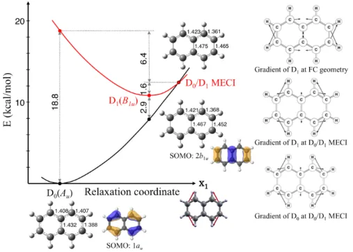
The results of our CASSCF and CASPT2 calculations are summarized in Figures 8, 9 and 10. Figures 8 and 9 show the CASSCF potential energy profiles of the three electronic states involved in the photophysics of the naphthalene cation. These states are the ground, D0(Au), and the first two
excited states, D1(B1u) and D2(B2g) (where the label Dn refers to the order obtained for vertical
transitions). The potential surface is displayed on two separate diagrams for clarity, because the reaction coordinate is not the same in both cases. All the optimized minima and crossings have D2h
point group symmetry and the structures are drawn up on these figures. The energy gradient vectors of the states at the Franck-Condon points and crossings are opposite to the forces acting on the molecule. These are shown to the right in Figures 8 and 9 to illustrate the driving force for the photophysics and the nature of the reaction coordinate, which is along the symmetry-preserving gradient difference vector (x1) in each case.
Figure 8. Optimized critical points of the naphthalene radical cation using CASSCF/6-31G* on the D0
and D1 states. Energies in kcal/mol. Vectors to the right display the energy gradients at the intersection
and FC geometry.
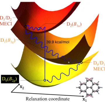
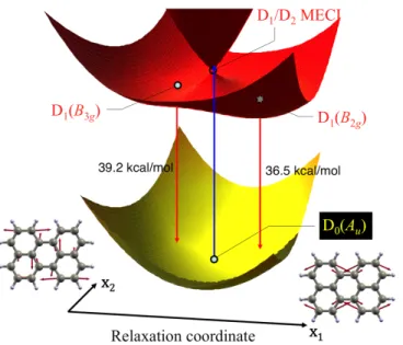
Figure 9. Optimized critical points of the naphthalene radical cation using CASSCF/6-31G* on the D1
and D2 states. Energies in kcal/mol. Vectors to the right display the energy gradients at the intersection
and FC geometry.
Upon excitation to the D2 state, the system will relax to the nearby D2 minimum. The initial forces
acting on the system correspond to the opposite of the gradient difference vector and points directly towards a D1/D2 MECI. This crossing is located over 20 kcal/mol above the D2 minimum however.
Upon nonradiative decay at the crossing region, the system further relaxes on the D1 PES. The forces
then drive the system directly towards the D1 minimum. Along the same direction is located an easily
accessible D0/D1 MECI less than 2 kcal/mol above this minimum. This funnel allows for a fast internal
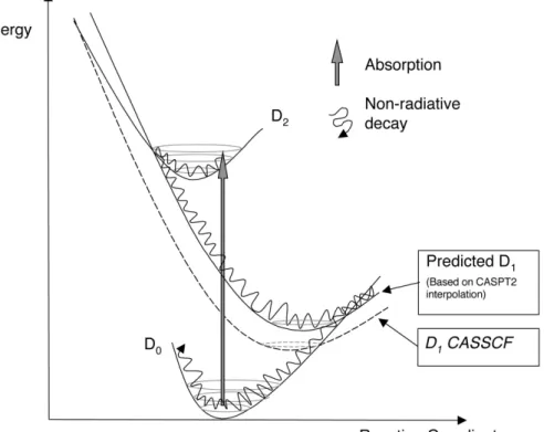
conversion back to the ground state. The photophysical mechanistic picture that emerges from these calculations is thus rather simple. It is illustrated in Figure 10. The efficient and ultrafast ground-state
recovery upon photoexcitation of N•+ results from easily accessible funnels between the populated electronic states. These funnels correspond to sloped conical intersections and the forces acting on the nuclei drive the system efficiently toward these funnels. Note however that, at the CASSCF level, the D1/D2 MECI is too high in energy to account for the ultrafast decay observed experimentally. Only at
the CASPT2 level is the picture in better agreement with the experimental measurements. Indeed, at this level of calculation, the D1/D2 MECI is lowered in energy relative to the D2 minimum energy.
This is a direct consequence of larger correlation energy in the D0 and D2 states compared to the D1
state.
Figure 10. Schematic representation of the electronic relaxation mechanism of the naphthalene radical cation. Dashed curve: original CASSCF/6-31G* result for D1 state. Solid curve: predicted relative
increase in D1 energies indicated by CASPT2 calculations, suggesting a lower energy D1/D2 MECI,
allowing for nonradiative relaxation.
It is remarkable to note that the photophysics of N•+ is very different from that of its neutral
counterpart. Neutral naphthalene (N) is known to exhibit mainly fluorescence in the near ultra-violet (UV) after photoexcitation to the S1 excited state.81 Like in benzene, it can probably undergo
photoisomerization reactions to produce valence isomers such as naphthvalene and/or benzofulvene. This is in contrast with the ultrashort excited-state lifetime observed in N•+. Figure 11 compares the
potential energy profiles of neutral and cationic naphthalene in the ground and first excited states. The S0→S1 vertical transition energy in N is much larger than the corresponding D0→D1 vertical transition
energy in N•+. This is expected based on the nature of the excited states. The S1 state of N results from
transitions between occupied π orbitals to unoccupied (virtual) π* orbitals (π→π* transitions), while the D1 state of N•+ results from a transition between occupied π orbitals (π→π transition). Therefore, it
is not surprising that the energy gap is much lower in the cationic species. Upon geometry optimization of the excited state, the structure remains highly-symmetric (i.e., D2h symmetry) both in
N and N•+. However, the energy gap with the ground state remains very large in N, while it is considerably reduced in N•+. As a consequence, crossing with the ground state can only occur in N
upon pyramidalization of a benzene ring, which is an activated process with a barrier of about 30 kcal/mol. Thus, unless the system has enough vibrational kinetic energy to overcome this barrier, the system will remain trapped in the S1 minimum until radiative decay (fluorescence) occurs. If the
excitation energy is high enough to provide the system with sufficient energy to overcome the barrier, then the S0/S1 conical intersection can be reached and nonradiative decay to the ground state becomes
efficient. The system can either return back to its original naphthalene structure, or, because of the peaked topology of the MECI, lead to new photoproducts corresponding to valence isomers. This behavior is very similar to the one observed in benzene (see Figure 1).
Figure 11. Comparison of the CASSCF potential energy profiles in the ground and first excited states of (a) neutral naphthalene and (b) naphthalene radical cation. The neutral PAH exhibits fluorescence or photoproducts formation depending on excitation energy, while the cationic PAH is highly photostable.
Pyrene cation. Regarding Py•+ no time-resolved photodynamics study has been reported so far.
Because this cation is often considered to be a strong candidate for one of the DIB carriers,82 we have
investigated the topological features of the relevant PESs for this system.79 The results are summarized
in Figure 12. The presence of two easily accessible sloped D1/D2 and D0/D1 conical intersections
suggests that Py•+ is highly photostable, with ultrafast nonradiative decay back to the initial
ground-state geometry predicted via a mechanism similar to the one found in N•+. However, the two funnels
involved are even more accessible in Py•+ compared to N•+, suggesting a shorter excited-state lifetime