HAL Id: tel-03200111
https://tel.archives-ouvertes.fr/tel-03200111
Submitted on 16 Apr 2021
HAL is a multi-disciplinary open access
archive for the deposit and dissemination of sci-entific research documents, whether they are pub-lished or not. The documents may come from teaching and research institutions in France or abroad, or from public or private research centers.
L’archive ouverte pluridisciplinaire HAL, est destinée au dépôt et à la diffusion de documents scientifiques de niveau recherche, publiés ou non, émanant des établissements d’enseignement et de recherche français ou étrangers, des laboratoires publics ou privés.
measurements-model approach
Grazia Maria Lanzafame
To cite this version:
Grazia Maria Lanzafame. Understanding organic aerosol formation processes in atmosphere using molecular markers : a combined measurements-model approach. Ocean, Atmosphere. Sorbonne Uni-versité, 2019. English. �NNT : 2019SORUS519�. �tel-03200111�
ED 129
INERIS
Understanding organic aerosol formation processes in
atmosphere using molecular markers: a combined
measurements-model approach
Par Grazia Maria Lanzafame
Thèse de doctorat de Chimie de l’environnement
Dirigée par Bertrand Bessagnet
Présentée et soutenue publiquement le 12/12/2019
Devant un jury composé de :
Mme D’ANNA Barbara, Directrice de recherche, LCE Mme HODZIC Alma, Directrice de recherche, LA
Mme SARTELET Karine, Directrice de recherche, CEREA Mme TURQUETY Solène, Maitre de conférences, UPMC
M. BALDASANO José Maria, Professeur, Université Polytechnique de Catalogne M. VILLENAVE Eric, Professeur, Université de Bordeaux
Mme CAMREDON Marie, Maitre de conférences, LISA M. COUVIDAT Florian, Ingénieur de recherche, INERIS M. ALBINET Alexandre, Ingénieur de recherche, INERIS
M. BESSAGNET Bertrand, HDR, Chargé d’Affaires Scientifiques, INERIS
Rapporteur Rapporteur Examinatrice Examinatrice Examinateur Invité Invitée Responsable de thèse Responsable de thèse Directeur de thèse
First of all I would like to thank all my supervisors, Bertrand, Olivier, Alex and Florian, for giving me the opportunity to do this PhD. Special thanks are due to Alexandre Florian. Alex, your scientific support was fundamental and the challenges you've put me up against have made me grow as a better scientists. Florian, you taught me everything I know about about modeling, with a lot of patience and a smile. You believed in me till the end, also when I was driving you crazy.
I wish to acknowledge Eric Villenave and Marie Camredon for their participation during my PhD Committees, providing always a fresh and interesting point of view on my job.
I am also grateful to Barbara D'anna and Alma Hodzic for accepting reviewing this manuscript and to the examiners Karine Sartelet, José Maria Baldasano and Solène Turquety. I would like to offer my special thanks to all the teams in which I worked during my PhD: - The ASUR/EMIS team: Marc and Caroline for their kindness and availability, Valerie and Marie for their smile and their patience, Laurent for his support in my mother tongue :), Tanguy for his philosophic discussions, François for the nice talks, Nicolas K. and Robin for their support during Landex (I would never have survived without your help!) and Adrien for his work during the EVORA campaign. I also would like to thank and all the other team members for the nice time spent together: Florence, Nathalie M., Nathalie B., Celine, Sebastien, Olivier L., Jessica Q., Virginie, Anne-Sophie, Serge, Isaline, Jean, Benedicte, Cecile R., Vincent F., Fabrice, Hugo, Sylvie, Marion, Warda and Aline.
-The ANAE team: Jérôme and his precious help with the GC (you are the master), Hervé for his collaboration during the EVORA campaign, Claudine C. and Faustina for their understanding and support, Serguei (you will always be the ASE god for me), Yohann, Farid, Azziz, François, Cecile L., Claudine D., Ahmad, Jean-Pierre, Sylvain, Nicolas C., Valerie, Arnaud and Hugues.
-The MOCA/EDEN team: Simone, Elsa, Cynthia, Pierre, Simon, Valentin, Alicia, Florence, Fred, Blandine, Antonio, Gaël, Anthony, Jessica and Augustin. Your good mood (and your beliefs on italian food) made easier my last year at INERIS (and you also taught me new french words ahah)
My special thanks go to my family abroad, my office mates: Deep and Yunjiang, I learn a lot from both of you and please never tell anybody what we were discussing when the office door was closed :D. Lei, I know that you are still crying since I left. Camilla, one of the best person I ever met.
I wish to thank also all the other students met during this journey for the nice time spent together: Eleonora and Jasmina,the only people I trust for cooking pasta in France, Alexandre "Perlana", Marta (best road trip EVER), Adrien (BBQ king), Anitha, Ibtihel, Thi Cuc, Quentin, Pierre, Manoj, Martin, Kevin, Hugo, Vincent, Victor, Anne-Sophie, Julien, Katia, Maria, Nihal and Andrea.
I would also like to thank my friends spread all over the word who listened to my infinite complains during the PhD. Don't worry, I will soon complain about my job.
Finally, I wish to thank my parents and my sister that are proud of me also if they didn't fully understand what I was working on. Thanks for your constant support and encouragement. I owe your everything.
Chapter I ... 1
Introduction and objectives of the Thesis ... 1
1.1. Atmospheric aerosols ... 2
1.1.1. Definition ... 2
1.1.1. Aerosol impacts on air quality and climate. ... 3
1.1.2. Air quality and air pollution policies ... 6
1.2. Aerosol chemical composition ... 7
1.2.1. Primary and secondary organic aerosol ... 7
1.2.2. SOA formation: precursors and their reactivity in atmosphere ... 8
1.2.3. Gas to particle partitioning of secondary compounds ... 11
1.2.4. Benefits of an aerosol molecular characterization ... 13
1.2.5. Source apportionment ... 15
1.2.6. Definition and use of OA markers in literature ... 16
1.3. State of art modelling secondary organic aerosol ... 18
1.3.1. Air quality model structure ... 18
1.3.2. SOA modelling approaches ... 19
1.3.2.1. Two-products model ... 19
1.3.2.2. VBS (Volatility Basis Set) approach ... 20
1.3.2.3. Molecular surrogate approach ... 20
1.3.2.4. Model performances ... 22
1.4. PhD thesis objectives ... 23
References ... 25
Chapter II:SOA markers measurements ... 37
Article I: One-year measurements of secondary organic aerosol (SOA) markers in the Paris region: concentrations, seasonality, gas/particle partitioning and use in SOA source apportionment ... 37
Abstract ... 40
1. Introduction and objectives ... 42
2. Experimental ... 44
2.1. Sampling site and sample collection ... 44
2.3. SOA markers analysis quality control/quality assurance...46
2.4. On-line measurements ... 46
3. OA source apportionment ... 47
3.1. SOA tracer method ... 47
3.2. Positive matrix factorization (PMF) ... 48
4. Results and discussion ... 48
4.1. SOA marker concentration levels and comparison with literature data...48
4.2. SOA marker temporal evolutions and seasonality...51
4.3. Focus on the October/November 2015 period ... 53
4.4. SOA markers gas/particle partitioning (GPP) ... 55
5. Conclusions ... 60
References ... 61
Supplementary Material ... 77
Chapter III: Model to measurements comparison: Anthropogenic markers ... 119
Article II: Modelling organic aerosol markers in 3D air quality model. Part 1: Anthropogenic organic markers. ... 119
Abstract. ... 122
1. Introduction and objectives ... 123
2. Model development ... 125
2.1 Overview of the marker mechanism ... 125
2.1.1 Marker GPP computation ... 126
2.2 Anthropogenic OA marker formation in the atmosphere: mechanisms and GPP parameters ... 128 2.2.1 Levoglucosan ... 129 2.2.2 Nitroguaiacols ... 129 2.2.3 Nitrophenols ... 130 2.2.4 DHOPA ... 131 2.2.5 Methyl-nitrocatechols ... 134 2.2.6 Phthalic Acid ... 135
3. Comparison measurements model ... 136
3.1 Configuration ... 136
3.2 Measurements ... 139
4. Results and discussion ... 140
4.1 Model to measurement comparison ... 140
4.1.1 Levoglucosan ... 140
4.1.2 Nitroguaiacols and nitrophenols ... 147
4.1.3 Methylnitrocatechols and DHOPA ... 148
4.1.3 Phthalic acid ... 151
4.1.4 Correlation between secondary markers and levoglucosan ... 151
4.2 GPP estimations ... 152
4.2.1 Levoglucosan: spatial variability and model sensitivity to thermodynamic assumptions ... 152
4.2.2 GPP of secondary markers at SIRTA. ... 155
4.2.3 Influence of partitioning and gas-phase dry deposition of secondary markers on total concentrations ... 158
4.2.4 Evaluation of the OA-tracer approach to evaluate the wood-burning OM: Analysis of OMwb pLEVO-1 variations ... 161
Conclusions ... 163
References ... 165
Supplementary Material ... 174
1. Introduction and objectives ... 200
2. Model overview ... 202
2.1 Development of the marker mechanism ... 203
2.1.1 α- and β-pinene markers ... 205
2.1.2 Isoprene markers ... 215
3. Comparison measurements model ... 217
3.1 Configuration: model resolution and domain ... 217
3.2 Measurements: SIRTA ... 218
4. Results and discussion ... 219
4.1 Model to measurement comparison ... 219
4.1.1 α-/β-pinene marker temporal variations ... 221
4.1.2 Isoprene marker temporal variations ... 222
4.2 Influence of chemical regime on total marker concentrations ... 224
4.2.1 α-/β-pinene markers ... 225
4.2.2 Isoprene markers ... 226
4.3 Pinonic acid formation process: spatial and daily variability ... 227
4.4 GPP estimations at SIRTA ... 230
4.4.1 Model to measurements comparison: a focus on thermodynamics. ... 230
4.4.2 Influence of partitioning and gas-phase dry deposition on total marker concentrations ... 232 Conclusions ... 235 References ... 237 Supplementary Material ... 246 References ... 251 Chapter V ... 253
Conclusions and perspectives ... 253
1. Molecular marker measurements and database ... 255
2. Molecular markers model/measurements comparison: knowledge of physicochemical processes and emissions ... 256
2.1 Knowledge of the emissions ... 257
2.2 Knowledge of the chemical processes ... 257
2.3 Gas/particle partitioning evaluation ... 259
3. Molecular markers for source apportionment ... 259
References ... 260
1
Chapter I
Introduction and objectives of the
Thesis
2
1.1. Atmospheric aerosols
1.1.1. Definition
Aerosols are defined as suspended solid and liquid particles in a gas. In atmospheric sciences, the term aerosol is commonly used to indicate particulate matter (PM), although the original definition of the term is referred to the gaseous and the particulate phase together.
Because of the variety of sources and processes associated to atmospheric aerosol production, their concentrations in the atmosphere vary widely regionally and seasonally. Primary aerosols are directly emitted as particles in the atmosphere by both, natural (mainly vegetation, oceans, soil resuspension, volcanoes) and anthropogenic (biomass burning, traffic exhaust, industrial activities, etc.) sources. Secondary aerosols are produced in the atmosphere as a result of physical and chemical transformations of gaseous phase compounds.
Atmospheric aerosols are classified according to their aerodynamical diameters that range from a few nanometres to several micrometres. The most widely used aerosol classes are named PM1, PM2.5 and PM10, which correspond respectively to particles with diameter
smaller than 1, 2.5 and 10 µm. Their size influences their half-life and transportation, health impacts and interactions with light.
A scheme of particle size distribution, together with the main production and removal processes associated, is presented in Figure 1.1. Fine aerosol fraction (PM2.5) includes the
Aitken nuclei and accumulation modes that are produced mostly from condensation of low volatility compounds and coagulation of smaller particles (ultra-fine particles). Their half-life in the atmosphere is about few days to two weeks (Kristiansen et al., 2016). These particles can either be removed from the atmosphere by dry and wet deposition or can continue to grow in size by coagulation with other particles or by condensation of low volatility compounds onto their surface(Pöschl, 2005). Most of the coarse particles (larger than 2.5 µm) are directly emitted in the atmosphere (Finlayson-Pitts and Pitts, 2009) by anthropogenic and natural sources, which includes resuspension of dust, primary biological particles (spores, pollens…) and sea spray. In the atmosphere, coarse particles are also formed by coagulation of smaller particles and low-vapor pressure compounds on their surface. Coarse aerosol half-lives range between some minutes to several days (Seinfeld and Pandis, 1998). Typical tropospheric particles concentrations are in the range of 102-105cm-3 in number and 1-100 mg m-3 in mass (Krejci et al., 2005; Raes et al., 2000; Van Dingenen et al., 2004; Williams et al., 2002).
3
Figure 1.1. Schematic representation of principal modes, sources and aerosol formation and
removal mechanisms. Adapted from:[Whitby and Sverdrup, 1980]
1.1.1. Aerosol impacts on air quality and climate.
Aerosols are getting growing attentions from the scientific community due to their proven effects on health, climate and visibility. According to the World Health Organization (WHO), 4.2 million people died because of air pollution in 2016 (WHO, 2018). Air pollution is considered as the largest environmental health hazard in Europe (EEA, 2018).
Several epidemiological studies proved the connection between particulate air pollution and an increment of respiratory diseases and adverse effect on cardiovascular system (Heal et al., 2012; Seaton et al., 1995) that can cause premature deaths (Apte et al., 2015; Burnett et al., 2018). Reduced lung function, respiratory infections and asthma have been recognized as effects of both acute and chronic exposure to air pollution. Recently, evidences of air pollution effects on diabetes, obesity, systemic inflammation and neurological diseases incidence have been also provided (RCP, 2016, and references therein; WHO, 2018).
4
Particle hazard depends on their size: coarse particles with a diameter between 10 and 30 μm are usually deposited in the oropharyngeal region, particles with dimensions between 2 and 16 µm can reach the terminal bronchioles and finer particles (< 2 µm) penetrate further till the alveolar sacs (Figure 1.2). Finer particles can interfere in the exchanges between air and blood, introducing toxic substances in the circulatory system. The most widely known toxic substances that can be absorbed on the aerosols are metals (Cu, Pb, Cd …), polycyclic aromatic hydrocarbons (PAHs), polychlorobiphenyls (PCBs) and dioxins (Finlayson-Pitts and Pitts Jr, 2000; Jacobson et al., 2000). Metals and PAHs are regulated in Europe by the European Directive 2004/107/CE (European official journal, 2004).
Figure 1.2. Airways of the adult lung and particle deposition in function of their sizes.
Adapted from: [Nahar et al., 2013]
Besides health impact, aerosols can scatter and absorb infrared and visible light, contributing to climate change. Three radiative forcing (RF) have been estimated for aerosol interactions with solar light: the aerosol-radiation interaction, the aerosol-cloud interaction and the impact of black carbon (BC) on snow and ice surface albedo (IPCC, 2018).
5
Aerosols mostly scatter solar radiation, leading to a cooling effect, and absorb solar radiation only when composed by absorbing components as black carbon (BC), causing a warming effect. The global RF estimate for the direct aerosol-light interaction is negative (-0.35 W m-2), with a prevalence of the scattering effect. Besides, aerosol–cloud interactions are usually considered as indirect effects of aerosol on climate. Reflecting properties and lifetime of clouds change according to aerosol sizes and composition (Haywood and Boucher, 2000), with consequences on the RF associated to cloud albedo. RF by aerosol effect contribution is highly uncertain, and rather a total effective radiative forcing (ERF), due to aerosol-radiation and aerosol-cloud interactions, has been calculated (-0.9 W m-2). Finally, the black carbon (BC) deposition reduces the snow and ice surface albedo, absorbing visible and ultraviolet light (RF +0.04). However, the contribution of this process is low compared to the previous ones.
Radiative forcing on climate between 1750 and 2011 is shown in Figure 1.3. Higher positive contributions to the total anthropogenic ERF are given by well mixed greenhouse gases (WMGHG), including CO2. Tropospheric ozone positive RF is in part compensated by the
stratospheric ozone negative RF. The only forcing agents giving significative negative ERF are aerosols-radiation and aerosol-cloud interactions. These effects mitigate but not fully contrast WMGHG ERF, and total balance of anthropogenic ERFs results positive.
6
Figure 1.3. Bar chart for radiative forcing (hatched) and effective radiative forcing (solid) by
concentration change between 1750 and 2011. Uncertainties (5 to 95% confidence range) are given for RF (dotted lines) and ERF (solid lines). Source: [IPCC, 2018]
1.1.2. Air quality and air pollution policies
Oxford dictionary defines air quality as ―the degree to which the air in a particular place is pollution-free‖. Industrialization and urbanization led to increasing emissions that modified the composition of the atmosphere. The consciousness about air quality monitoring importance has begun after the well-known acute pollution episodes of ―Los Angeles smog‖ (1949) and ―London fog‖ (1952). Pollution episodes usually occur when large amounts of pollutants are emitted in conditions of weak atmospheric dispersion. During severe pollution episodes respiratory disease incidence increase and excess mortality has been registered. Thus, in order to protect populations, concentrations of PM in ambient air are regulated, for example, in France and Europe by the European Directive 2008/50/EC (European official journal, 2008), which set concentration limit values for PM on annual (40 and 25 µg m-3 for PM10 and PM2.5 respectively) and daily (50 µg m-3 for PM10) timescale and with a maximum
number of exceedances over the calendar year (35 days per year). However, many studies shown that there is probably no PM concentration threshold below which no health impacts would be observed (WHO, 2017).
The knowledge of PM, and especially of the organic fraction, sources is essential for policy makers to apply efficient emission regulation policies. This can be achieved from measurements as nowadays, several monitoring networks are operational and perform continuous measurements of regulated pollutants, as PM2.5 and PM10, together with a detailed
aerosol chemical speciation. As an example, in France, air quality monitoring network is coordinated by the Central laboratory of air quality monitoring (LCSQA) in collaboration with the Official Air quality Monitoring Associations (AASQA) and several PM source apportionment studies have been performed in different locations (Weber et al., 2019). Air quality models are also widely used to forecast the air quality and help institutions to mitigate their effects. Daily air quality in France is forecasted with the air quality system Prev’Air (www.prevair.org). In addition, chemistry-transport models can also be used to apportion PM sources and have been applied in Europe during several studies (Brandt et al., 2013; Karamchandani et al., 2017; Skyllakou et al., 2014; Yang et al., 2019). Further details on source apportionment methodologies are given in section 1.2.5.
7
1.2. Aerosol chemical composition
Aerosols are constituted from both an inorganic and an organic fraction. The mineral fraction is dominated by sulfate, nitrate and ammonium and account for 40 to 60% of PM1 dry mass,
according to the kind of site considered (urban, urban background or rural) (Putaud et al., 2004; Zhang et al., 2011). OA fraction can account up to 90% (Kanakidou et al., 2005; Zhang et al., 2007, 2011) of particulate matter (PM) in ambient air (Figure 1.4). OA concentrations and compositions show large seasonal and regional variabilities and the knowledge of their sources and processes remain still poorly understood. OA is usually estimated by multiplying concentrations of OC with factors ranging from 1.5 to 2, depending on the assumed average molecular composition (Gelencsér et al., 2007; Russell, 2003). The use of a fixed factor to convert OC to OA may be insufficient to achieve high accuracy results (Brown et al., 2013). Only the identification and quantification of all OA components could make OA mass estimation possible. OA composition is extremely varied and variable and the most comprehensive OA characterization studies succeed in identifying only 10-40% of total OA (Pöschl, 2005).
Figure 1.4 Average chemical composition of PM1 for different types of site. Pink: chloride;
Yellow: ammonium, Blu: nitrate; Red: sulfate; Green: organic matter; Light green: oxygenated organic aerosol (OOA) equivalent to SOA (secondary organic aerosol) estimation; Grey: primary organic aerosol (POA). Adapted from [Zhang et al., 2011].
1.2.1. Primary and secondary organic aerosol
Primary organic aerosols (POA) are directly emitted into the atmosphere by the combustion of biomass and fossil fuels, sea spray and resuspension of biological (plant debris, pollen, fungal spore, etc.) and anthropogenic dusts. Secondary organic aerosols (SOA) are produced in the atmosphere via gas-to-particle conversion processes of semivolatile organic compounds
8
(SVOCs) (Hallquist et al., 2009) and account for a significant part (20-80%) of total OA (Jimenez et al., 2009; Kroll and Seinfeld, 2008; Srivastava et al., 2018; Zhang et al., 2007, 2011). Unlike primary particles, directly emitted into the atmosphere from characterized sources, secondary aerosols, including SOA, are difficult to regulate and technological constraints restrict their monitoring. A schematic representation of the processes involved in SOA formation is reported in Figure 1.5. Gaseous phase precursors are oxidized by homogeneous and heterogeneous reactions, giving low volatility compounds. These products can nucleate into new particles or condensate onto pre-existing particles. The new-born particles can keep growing by condensation processes and coagulation with other particles.
Figure 1.5 . Major microphysical and chemical processes that influence the size distribution
and chemical composition of atmospheric aerosol particles. Source: [Brasseur et al., 2003]
1.2.2. SOA formation: precursors and their reactivity in atmosphere
VOCs sources are from both, natural (plant emission, forest fires…) and anthropogenic (traffic, industrial activities and domestic heating emissions) origins. The processes leading to SOA formation from VOCs are complex and still poorly understood. For this reason, numerical models generally underestimate the SOA fraction (Bessagnet et al., 2008). Once emitted into the atmosphere VOCs undergo (photo-) oxidation through photolysis and reaction with OH, NO3 or O3. VOCs oxidation pathways occur through several steps, leading
to the formation of more functionalized, less volatile and more hydrophilic compounds. These chemical species partition onto the particle phase to form SOA until reaching thermodynamic
9
equilibrium. In the particle phase, SOA components can undergo further chemical (e.g. oligomerization) and physical (e.g. desorption, solubilization) processes.
Plant-emitted SOA biogenic precursors include isoprene, monoterpene and sesquiterpenes. The double C=C bonds contained by all these compounds can react with the main atmospheric oxidants (OH, NO3 and O3) (Calogirou et al., 1999). Monoterpenes have been
identified as the major biogenic SOA precursor (Guenther et al., 1995), with a global estimated contribution between 10 and 30% to total SOA (Pye et al., 2010; Spracklen et al., 2011; Tsigaridis and Kanakidou, 2003). Isoprene SOA yields has been estimated to be low (~1%) (Carlton et al., 2009; Kroll et al., 2006). However, isoprene is the largest non-methane VOCs compound emitted (600 Tg yr-1) on global scale (Guenther et al., 2006) and isoprene SOA can account for a maximum 30% to total OA (Heald et al., 2008). Sesquiterpenes have lower emissions than isoprene and monoterpenes (Acosta Navarro et al., 2014), but because of their high SOA yields they may contribute significantly to the biogenic SOA budget (Griffin et al., 1999).
Anthropogenic SOA precursors are mainly aromatic compounds (toluene, naphthalene, benzene, phenols, xylene, alkylbenzenes and PAHs) and long chain (number of carbons > 7) aliphatic alkanes (Bruns et al., 2016; Zhao et al., 2014). Their oxidation is initiated by reaction with OH, with SOA yields ranged from a few percent (Li et al., 2016; Ng et al., 2007) for aromatic compounds to 90% (Aumont et al., 2005; Lim and Ziemann, 2005, 2009) for long chain alkanes. Anthropogenic VOCs global emissions have been reported to be around 10% of total non-methane VOCs emissions (Goldstein and Galbally, 2007; Heald et al., 2010), but can become important locally in urban environments.
A schematic representation of a generic VOC oxidation pathway is reported on Figure 1.6. VOC oxidation is initiated by the reaction with an oxidant (OH, NO3 or O3) or by photolysis.
The produced alkyl radical (R) reacts then with a molecule of oxygen, becoming an alkyl-peroxyradical (RO2). RO2 fate depends on the NOx regime. At high-NOx conditions RO2 can
be oxidized by NO or NO2, to give in the first case, the correspondent alkoxy radical (RO) or
to the correspondent nitrate (RONO2) and in the second case, the peroxynitrate (ROONO2).
At low NOx concentrations, the reactions with HO2 and RO2 become possible, forming stable
products (hydroperoxydes, carboxylic acids, peroxyacids, alcohols and carbonyls) and RO radicals only for the RO2+RO2 reaction. RO undergoes isomerization or decomposition to
form a stable compound. The stable compounds produced (first generation oxidation products) can be further oxidized in gas phase (producing different generation on oxidation products), following the same scheme, or can partition onto the particulate phase (organic or
10
aqueous phases). These compounds, less volatile than VOCs, are named semi-volatile organic compounds (SVOCs). SVOCs gas/particle partitioning (GPP) is discussed in the next section.
Figure 1.6 VOC atmospheric degradation reactions proceeding through formation of an alkyl
11
Figure 1.7. Schematic description of bulk aqueous chemical processes involved in aqueous
SOA (aqSOA) formation. The same fundamental chemical mechanism applies for cloud droplets and aerosol water, however the dominant reactions differ due to differences in the chemical environment (pH, inorganic, and organic concentrations). Source: [McNeill, 2015] The main reactions involving water-soluble organic compounds (WSOC) in the aqueous phase are (Figure 1.7):
- dark reactions, as hydration, hydrolysis, self-oligomerization and ionization,
- the radical oxidation by OH, HO2, SO4 and HSO4, that generates organic acids or
organosulfates. At high WSOC concentrations the organic radicals created may react together to form oligomers.
- ionic reactions operated mostly by NH4+, SO42- and HSO4-. Organosulfates and
light-absorbing species are produced.
- photochemical reactions: photolysis of photolabile species and activation of photosensitizers (e.g. humic and fulvic acids).
Due to the different composition of aqueous aerosol phase and cloud water, the expected predominant reactive pathways for aqueous phase SOA formation (aqSOA) are different in both media (McNeill et al., 2012; Tan et al., 2010). In the aerosol aqueous phase (0<pH<3 (Freedman et al., 2019), rich in organics and supersaturated in salts) acid-catalysed reactions and inorganic−organic reactions and oligomerization are favoured. In cloud water (pH>3, less concentrated organics and salts), OH oxidation mechanism predominates.
1.2.3. Gas to particle partitioning of secondary compounds
SVOCs partition between gas-phase and the aqueous and organic phases of aerosols, generating SOA. The volatility of chemical species is directly proportional to their saturation vapor pressure, defined as the pressure at which the vapor of the compound is at the equilibrium with its solid (solid saturated vapor pressure) or liquid (liquid or subcooled saturated vapor pressure) phase. Saturated vapor pressure depends on temperature following a Clausius-Clapeyron relation: at higher temperatures saturated vapor pressure decreases, determining a particulate phase fraction decrement. According to Raoult’s law the concentrations in the liquid phase and in the gas phase at equilibrium are linked by the following relation:
12
where Pi is the partial pressure of the compound i in the gaseous phase, xi the molar fraction
of the compound i in the liquid phase, Pi0 is the compound saturated vapor pressure of i and
γG,i and γL,i are the activity coefficients respectively in the gaseous and the liquid phase.
Activity coefficients indicate the interactions between the different species in solution. When ideality is assumed, all the interactions between the mixture components are assumed identical and therefore all the activity coefficients values are taken equal to 1. Raoult’s law then become:
𝑃𝑖 = 𝑥𝑖𝑃𝑖0 (Eq 1.2) This version of Raoult’s law is commonly used to describe the gas to particle partitioning in air quality models. However, if atmospheric gases behavior can be assumed as ideal (as gases behavior is ideal at pressures far below the atmospheric pressure), this is not the case for the aerosol phase. The Raoult’s law form to calculate gas/particle this equilibrium can be written as follows:
𝑃𝑖 = 𝛾𝐿,𝑖𝑥𝑖𝑃𝑖0 (Eq 1.3)
in which only the liquid phase activity coefficients are taken in account.
A modified version of the Raoult’s law to calculate the partitioning between the gaseous and the organic phases has been proposed by (Pankow, 1994):
𝐾𝑝,𝑖𝑀0 =𝐴𝑝 ,𝑖
𝐴𝑔,𝑖 (Eq 1.4) Where 𝐾𝑝,𝑖 is the gas-particle partitioning constant (m3 µg-1), 𝐴𝑝,𝑖 is the organic phase concentration in µg m-3 and 𝐴𝑔,𝑖 and 𝐴𝑝,𝑖 are respectively the concentrations of the component
i in the gas and in the particulate phase. This model assumes that the particulate phase of organic aerosol is constituted by a single and homogeneous phase, which is not the case for the real aerosols. 𝐾𝑝,𝑖 is linked to the saturated vapor pressure by the following relation:
𝐾𝑝,𝑖 = 760×𝑅×𝑇
𝑀𝑜𝑤𝛾𝑖106𝑃𝑖0
(Eq 1.5) where the temperature (T) is expressed in K, R is the perfect gas constant (8.206×10⁻⁵m3 atm mol-1 K-1), 𝑀𝑜𝑤 is the molar mass of the organic phase in g mol-1 and the saturated vapor pressure (𝑃𝑖0) is in torr.
For diluted solutions, the partitioning between the gaseous phase and the aqueous phase can be computed using Henry’s law:
13
where 𝐶𝑖, 𝐻𝑖 and 𝑃𝑖 are respectively the aqueous phase concentration, the Henry’s law constant (mol L-1 atm-1) and the molar partial pressure of i. In conditions of infinite dilution (𝐶𝑖 → 0), Henry’s law and Raoult’s law can be combined:
𝐻𝑖 = lim𝐶𝑖→0 𝐶𝑖
𝑃𝑖 =
𝜌𝑤𝑎𝑡𝑒𝑟
𝑀𝑤𝑎𝑡𝑒𝑟 ×𝛾𝑖∞×𝑃𝑖0
(Eq. 1.7) in which 𝜌𝑤𝑎𝑡𝑒𝑟 is the water density (g L-1), 𝑀𝑤𝑎𝑡𝑒𝑟 is the water molar mass (g mol-1) and 𝛾𝑖∞
is the infinite dilution activity coefficient of the substance i in pure water:
𝛾𝑖∞ = lim𝑥𝑖→0 𝛾𝑖 𝑥𝑖 (Eq. 1.8) 𝛾𝑖∞ represents the activity coefficient of i when it is surrounded only by water. Henry’s law constant takes in account both the compound volatility (𝑃𝑖0) and its affinity with water (𝛾
𝑖∞).
In real conditions, aerosol aqueous phase is not pure, and the compounds are not infinitely diluted. A relative activity coefficient can be calculated by the ratio of infinite dilution and liquid phase activity coefficient:
𝜁𝑖 = 𝛾𝑖
𝛾𝑖∞ (Eq. 1.9)
To compute gaseous to aqueous phase partitioning in the aerosol aqueous phase (no infinite diluted phase) Raoult’s law can be rewritten:
𝐶𝑖 = 𝐻𝑖×𝑃𝑖
𝜁𝑖 (Eq. 1.10)
Following the model proposed by Pankow, (1994) for the partitioning with the organic phase, an analogous gas-water partitioning coefficient, 𝐾𝑎𝑞 ,𝑖 (m3 µg-1), can be defined:
𝐾𝑎𝑞 ,𝑖𝐿𝑊𝐶 =𝐴𝑎𝑞 ,𝑖
𝐴𝑔,𝑖 (Eq. 1.11)
in which LWC is the liquid water content (µg m-3) and 𝐴𝑎𝑞 ,𝑖 and 𝐴𝑔,𝑖 are respectively the concentrations in aqueous and gaseous phases. Equation 1.11 can be rewritten in function of Henry’s law constant:
𝐾𝑎𝑞 ,𝑖 = 𝐻𝑖×𝑅×𝑇
𝜌𝑤𝑎𝑡𝑒𝑟 𝜁𝑖×1.013×10¹¹ (Eq 1.12)
1.2.4. Benefits of an aerosol molecular characterization
The characterization of the SOA composition and more generally OA has been a subject of great scientific interest in the recent years. A better knowledge of OA chemical composition is necessary to apportion OA sources and plan strategies for emission reduction. An improvement in air quality requires an understanding of the composition of ambient aerosols
14
and their major sources. Other reasons for this interest are related to the potential impacts of organic molecules on health (e.g. PAHs) or on climate (e.g. light-absorbing molecules and CCN activity) and on the particle formation processes (e.g. volatility and partitioning). OA major components, together with their sources, are reported in Table 1.1. The proportions reported are only indicative, since aerosol chemical composition varies considerably according to the season and the region considered.
Organic aerosol chemical characterization is usually performed on PM samples collected on filters. PM samples are extracted with solvents, selected according to the targeted compounds, or by thermal or laser desorption systems coupled with an analytical instrument. Analyses are performed using chromatographic separation and detection instruments, such as gas or liquid chromatography-mass spectrometry (GC or LC-MS). Online techniques (e.g. aerosol mass spectroscopy, AMS) are also used to deduce the OA degree of oxygenation, with no information on the identity of the individual compounds. As can be inferred from Table1.1, some substance classes are typically from specific sources (e.g. sugars for biomass burning) and others may indicate the aerosol age (e.g. highly functionalized molecules as dicarboxylic acids). Specific molecules from these classes have been identified and used as molecular markers for source apportionment. Organic markers can be later used for source apportionment using statistical source-receptor models as described in the following section.
15
1.2.5. Source apportionment
Source apportionment can be performed using source-receptor models (PMF, CMB…), based on measurements (Srivastava et al., 2018), or by chemistry transport models (CTMs) (Burr and Zhang, 2011; Wagstrom et al., 2008; Zhang, 2005), for which general features are presented in section 1.3.1.
Source-receptor models are based on the solution of the mass balance equation. To apply these methods, the assumptions done are: (1) stable and reproducible source profile, (2) non-reactive and non-volatile receptor species, (3) receptor data representative of the geographical area studied and (4) quantification of receptor and sources has been performed with equivalent or comparable methods throughout the period considered. The chemical mass balance (CMB) only considers primary sources because the determination of profiles for secondary sources is difficult to be obtained. Thus, the OA not apportioned refers to SOA. SOA is then defined as the difference between the measured OA concentrations and the aggregated OA concentrations from all primary sources resolved by CMB. In positive matrix factorization (PMF), SOA is commonly calculated as the sum of OA loadings associated to sulfate- and nitrate-rich factors. By comparison, molecular organic markers (tracers) are source-class specific and may provide a more definitive link between factors and source classes. Molecular markers for SOA and POA can be directly included in the PMF model providing an insight into the primary–secondary split of OA sources. The effectiveness of the method depends on the molecular markers used. Besides, the SOA-tracer method developed by Kleindienst et al., (2007) allows the estimation of the SOA contributions from several biogenic and anthropogenic hydrocarbon SOA precursors to ambient OC concentrations using a series of organic molecular compounds called tracer (or marker) compounds. The SOA tracer method is based on the estimation of the SOA mass contribution using marker measured concentrations and SOA-to-marker mass fractions determined by chamber experiment. A comparison on the different existing methods to apportion SOA from filter measurements, and notably both used in this work namely PMF and SOA tracer-method, can be found in Srivastava et al., (2018). Further details on PMF and SOA tracer method are provided in Chapter II.
Two approaches are commonly used for source-oriented modelling techniques with CTMs: the brute force method (BFM) and the tagged species method (Belis et al., 2019). BFM consist in a sensitivity analysis on emission sources contributions on total PM. Emissions
16
from a specific set of sources can be modified, either by sectors or by geographical regions. The comparison with a baseline run, performed with unperturbed emissions, is required to quantify the contribution of that specific source. The relation between precursor emission and PM concentrations include non-linear effects, because of the contribution of SOA formation in atmosphere. The tagged species method quantifies the source contribution using extra-species, known as ―reactive tracers‖, that undergo chemical transformation in atmosphere generating secondary products. This method is based on a conservative mass approach, in which the sum of all the secondary product concentrations is equal to the total concentration of the sources (Yarwood et al., 2007).
1.2.6. Definition and use of OA markers in literature
A good aerosol source tracer should fulfil the following requirements: (1) to be unique to the source of origin, (2) to be produced in reasonably high yields so at sufficiently high concentrations in the atmosphere to allow for reliable quantification, (3) to be reasonably stable in the atmosphere, so that it is conserved between emission/formation and collection at a receptor location (4) to have a low vapour pressure so that it primarily partitioned to the particle phase, which minimizes possible underestimation from loss to the gas phase (Al-Naiema and Stone, 2017; Sheppard, 1963). All these conditions are rarely satisfied, so the term ―marker‖ is more appropriate to define these species. In fact, recent studies demonstrated that most of the tracer lifetimes are in the range of couple of days (e.g. levoglucosan 0.7-2.2 days (Hennigan et al., 2010), pinonic acid ~2.1–3.3 days (Lai et al., 2015) and MBTCA ~1.2 days (Kostenidou et al., 2018)), which is shorter than the average particle half-life of 1 week (Seinfeld, 2015). Therefore, their use in source-receptor models for source apportionment may cause an underestimation of the source contributions (Robinson et al., 2007).
Commonly used POA markers include: levoglucosan for biomass burning (Simoneit et al., 1999), hopanes for vehicular exhaust (Lough et al., 2007) and odd carbon C29-C33 n-alkanes from vegetal detritus (Rogge et al., 1993).
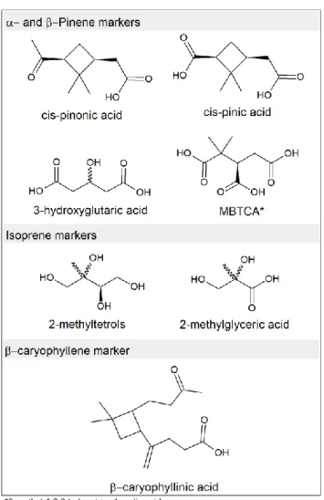
SOA markers from both biogenic and anthropogenic sources have been identified and reported in the literature. Monoterpene (α- and β-pinene) SOA markers include multifunctional carboxylic acid, among which the most well-known and studied are pinonic acid, pinic acid, 3-methyl-1,2,3-butanetricarboxylic acid, 3-hydroxyglutaric acid and terpenylic acid (Claeys et al., 2007, 2009; Hoffmann et al., 1998; Szmigielski et al., 2007; Yu et al., 1999). MBTCA and 3-hydroglutaric have been identified as marker for aged SOA (or
17
second generation oxidation markers) (Claeys et al., 2007; Müller et al., 2012; Szmigielski et al., 2007). Isoprene SOA markers are methyltetrols, α-methylglyceric acid, C5 alkene triols
and their corresponding sulfate esters and nitrate esters (Claeys et al., 2004; Surratt et al., 2006). Methyltetrols are specific to low NOx conditions, while α-methylglyceric acid is
produced at high NOx concentrations (Surratt et al., 2010).The most widely used marker for
β-caryophyllene is β-caryophyllinic acid (Jaoui et al., 2007) (Figure 1.8).
Figure 1. 8 Structures of some biogenic SOA markers divided by their precursor.
Several anthropogenic SOA markers from benzene, toluene, naphthalene and phenolic compounds oxidation have been identified (Figure 1.9). These markers are however less source specific than the biogenic ones, because their precursors can be emitted from several sources and most of them are also directly emitted. The most widely known tracer for toluene photooxidation is the 2,3-Dihydroxy-4-oxopentanoic acid (DHOPA) (Kleindienst et al., 2004), for which the formation mechanism in atmosphere has not been highlighted yet.
18
Phthalic acid is a tracer for naphthalene and methylnaphthalene photooxidation (Kleindienst et al., 2012) that can be also primarly emitted (Kawamura and Kaplan, 1987). Nitrated phenols and their methyl and methoxy derivatives are commonly recognized as secondary biomass burning markers (Forstner et al., 1997; Iinuma et al., 2010; Lin et al., 2015), although nitrophenols and methyl-nitrophenols have been measured also in primary emissions (Lu et al., 2019; Mkoma and Kawamura, 2013).
Figure 1. 9Structures of some anthropogenic SOA markers divided by their precursor. 1.3. State of art modelling secondary organic aerosol
1.3.1. Air quality model structure
Air quality models are a powerful tool to understand atmospheric processes, forecast and monitor air quality. These models, commonly called ―chemistry transport models‖ (CTM), use a mass conservative approach to reproduce pollutant chemical transformations and transport. The simulation domains are divided horizontally and vertically in a 3D mesh. In each box (cell) of this mesh all the variables (e.g. pollutant concentration, temperature, etc.) are homogeneous. CTMs require meteorological data, biogenic and anthropogenic emissions,
19
land use and topographic data, initial and boundary conditions, and embedded modules to solve chemical, thermodynamical and physical processes (Figure 1.10).
Figure 1.10 Schematic representation of a 3D chemistry transport model (CHIMERE). [c]mod
and [c]obs are respectively the modelled and the observed chemical concentrations field.
Adapted from: [Menut et al., 2013]
1.3.2. SOA modelling approaches
Simplified parametrizations to model secondary organic aerosol formation in the 3D CMTs have been developed, with the purpose to minimize computational costs. This kind of approach is useful for operational applications but is not sensitive to all the variations of atmospheric conditions. A brief description of the principal models used to represent SOA formation in CTMs is provided in the following paragraphs.
1.3.2.1. Two-products model
Odum et al., (1996) developed a method to parametrize secondary aerosol formation from a specific precursor using chamber experiment data. For each precursor, the fractional aerosol yield (Y) is calculated as follow:
𝑌 = Δ𝑀0
Δ𝑅𝑂𝐺 (Eq. 1.13)
where Δ𝑀0 is the concentration of the organic aerosol mass (µg m-3) produced and Δ𝑅𝑂𝐺 is
20
The overall SOA yield is given by the sum of the single product yields, calculating their partitioning as proposed by Pankow, (1994):
𝑌 = 𝑀0 𝛼𝑖𝐾𝑜𝑚 ,𝑖
1+𝐾𝑜𝑚 ,𝑖𝑀0
𝑖 (Eq. 1.14)
where 𝛼𝑖 is the stoichiometric coefficient and Kom,i is the partitioning coefficient of each
product i. Chamber experiments data are fitted to find the best combinations of 𝛼𝑖 and Kom,i
that represent the SOA mass formed. The so-developed Secondary Organic Aerosol Module (SORGAM) has been first coupled to the EuroRADM CTM, considering aromatics, higher alkane and alkenes, pinene and limonene as SOA precursors (Schell et al., 2001).
1.3.2.2. VBS (Volatility Basis Set) approach
This approach consists in dividing semi-volatile organic compounds in classes (―bins‖), according to their volatility. Compound volatility is evaluated through their saturation concentration (𝐶𝑖∗), that is linked to the saturated vapor pressure (𝑃
𝑖0) with the following
relation:
𝐶𝑖∗ =𝛾𝑖𝑀𝑤
𝑅𝑇 × 𝑃𝑖
0 (Eq 1.15)
In the classic VBS approach, each volatility bin is treated as a unique compound regarding partitioning properties and reactivity. The compounds belonging to the same bin undergo a unique aging process, generating only bins of less volatile compounds.
This approach was developed initially to describe the partitioning of semi-volatile compounds in atmosphere (Grieshop et al., 2009; Robinson et al., 2007; Shrivastava et al., 2008). Afterwards, VBS approach has also been applied to develop parametrization of VOCs aging to form SOA (Hodzic et al., 2010; Tsimpidi et al., 2010). The oxidation is usually simulated using the same kinetic constant for all the bins, 4×10-11 cm3 molecule-1 s-1, validated by comparison with measurements (Shrivastava et al., 2008). An evolution of the traditional VBS approach is the VBS-2D, in which the bins are characterized also by their oxidation degree (O:C ratio). This implementation of the traditional VBS enables to diversify the SOA composition and reactivity (Donahue et al., 2011, 2012).
1.3.2.3. Molecular surrogate approach
The main feature of this approach is the choice of molecular surrogates to represent the total SOA mass (Pun et al., 2002, 2006; Pun and Seigneur, 2007). Few molecules, identified among the major photooxidation products of a specific precursor, are chosen as molecular
21
surrogates based on their volatility. The advantages of this approach rely on the possibility to use molecular surrogate structures to calculate their activity coefficient, with the UNIversal Functional group Activity Coefficient; (UNIFAC, Fredenslund et al., 1975) and to simulate aerosol non-ideality.
The hydrophilic/hydrophobic organic (H2O) (Couvidat et al., 2012) mechanism has been developed with this approach, considering isoprene, monoterpenes, sesquiterpenes, toluene and xylene as precursors and it has been implemented in the 3D models Polyphemus and CHIMERE. This mechanism uses both hydrophilic (acidic or undissociated species) and hydrophobic surrogates to represent biogenic SOA and only hydrophobic surrogates to represent anthropogenic SOA (see Table 1.2).
Table 1. 2. Properties of the SOA surrogate species used in H2O. Adapted from: [Couvidat et al., 2012]
The chemical scheme used to reproduce the surrogate formation is based on experimental studies and is sensitive to high and low NOx conditions. For some biogenic compound also
the oligomerization processes are taken into account.
POA are represented in this model as SVOCs. POA are splitted in three classes of volatility, POAlP, POAmP and POAhP, from the less to the most volatile. These classes have been determined by the fitting of the diluition curve of POA from diesel exhaust in Robinson et al., (2007) and represent respectively 25%, 32% and 43% of the "non-diluted" POA emissions. Each surrogate has a partitioning constant and default structures have been assigned to these surrogates to calculate their activity coefficients. Following Grieshop et al., (2009), POAlP,
22
POAmP and POAhP aging is simulated by reaction with OH and lead to a decrease in volatily by a factor 100. This parametrization assumes that the POA composition is constant, while it is well known that it changes according to the emission source. Although this is the main limitation of this mechanism, no exhaustive data on POA composition are available to develop an accurate parametrization for POA.
1.3.2.4. Model performances
Air quality models often underestimates SOA formation in the atmosphere. Several studies have been performed to estimate 3D CTMs performances. Tsigaridis and Kanakidou, (2003) focused on the simulation of the global SOA distribution, identifying some critical physicochemical processes in SOA modelling: the potential irreversibility of the partitioning onto the particle phase, the simulation of the aerosol mass on which SVOCs condense and the temperature dependence of the partitioning coefficients. Multiple intercomparison exercises have been performed on regional scale (Bessagnet et al., 2016; McKeen et al., 2007; Mircea et al., 2019; Pernigotti et al., 2013; Prank et al., 2016; Solazzo et al., 2012; Vautard et al., 2007). Solazzo et al., (2012) in the Air Quality Model Evaluation International Initiative (AQMEII) compared 10 air quality model outputs and none of them succeeded to represent PM10 mass
throughout the year. They attributed the underestimation of PM10 to a misrepresentation of
organic aerosol concentrations. Prank et al., (2016) identified the lack of precursor emissions from wildland fires and explicit representation of aerosol water content as the main reasons for PM10 underestimation in air quality models. Concerning the EURODELTA III
intercomparison exercise (Bessagnet et al., 2016; Mircea et al., 2019), similar performances related to the SOA modelling approach have been found (VBS vs SORGAM), with the difference that the VBS captured better the seasonal variations. SOA underestimation was attributed to a missing precursor emissions and SOA formation processes.
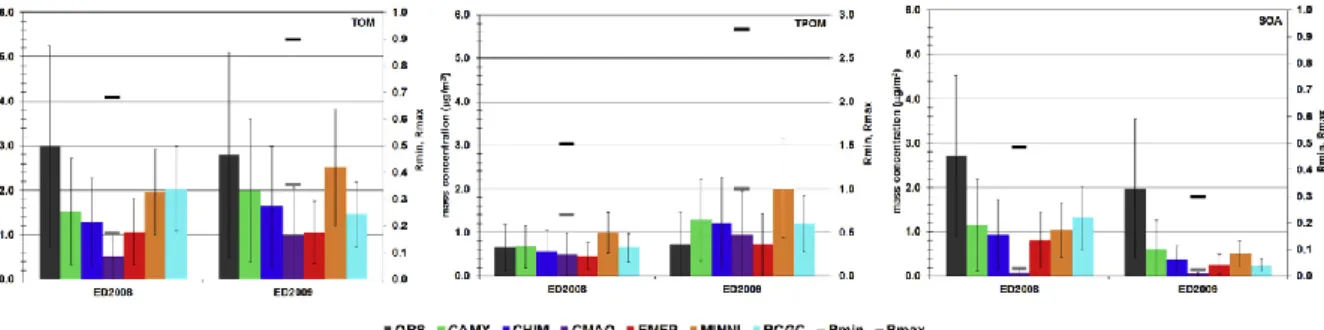
Figure 1. 11 From EURODELTA III intercomparison exercise: Comparison between
23
and secondary organic aerosol (SOA) concentrations (μg m−3) using 6 models (CAMX, CHIMERE, CMAQ, EMEP, MINNI and RCGC). Source: [Mircea et al., 2019]
The validation of the model outputs is normally achieved by comparison with measurements of oxidant concentration (e.g. O3), meteorological parameters (T, wind speed etc.) and PM
and carbonaceous species (EC/OC). However, compare directly the PM concentrations measured with the model output could be problematic because of the complex composition of the organic fraction.
1.4. PhD thesis objectives
A better knowledge of OA sources is required to apply efficient policies to mitigate pollution effects. As previously discussed, organic marker measurements are commonly used in source-receptor models to apportion OA sources. Source apportionment is also performed using CTMs, in which OA is often underestimated. Such underestimation increases with the photochemical aging of air masses, highlighting the incomplete identification of all SOA precursors and the poor knowledge of the processes involved in particle aging. The aim of this work was to implement a marker modelling approach in a 3D air quality model (CHIMERE). The ability of the model to reproduce marker concentrations observed in the ambient air is indicative of the model performances in representing the overall OA and SOA concentrations. Molecular markers are emitted and produced by the same sources and physicochemical processes of the organic aerosol bulk. A fair representation of the marker in a 3D CTM, could further allow to apportion OA sources using a hybrid CTM/Source-receptor model approach (Habermacher et al., 2007). The marker-implemented version of CHIMERE has been developed adding to the aerosol module detailed mechanisms for marker formation and improving emission inventories. Simulation outputs have been compared with measurements. The discrepancies observed have been investigated considering the possible model uncertainty, including primary emissions, chemical reactivity and GPP parameterization. This PhD manuscript is divided in 4 chapters. The main results, together with the methods used, are presented in 3 scientific articles:
- In Chapter II (Article 1) the annual measurements of biogenic and anthropogenic SOA markers performed at the SIRTA facility (25 km SW of Paris city centre) during 2015 (every third day) are shown. Literature data are provided for comparison with SOA
24
markers concentrations measured at SIRTA. The seasonal variations of 25 SOA marker concentrations and gas/particle partitioning are examined and discussed. SOA sources have been also apportioned using the SOA tracer method and the results obtained are compared with PMF outputs. This work constituted also the validation basis of the model developments made to simulate OA marker concentrations using CHIMERE. My contribution to the work presented in this chapter includes the development of the analysis method for the SOA markers in gaseous and particulate phase and the analysis of SOA markers in the gaseous phase.
- In Chapter III (Article 2), the primary emissions of levoglucosan, together with the formation mechanisms of 5 anthropogenic SOA markers (nitrophenols, nitroguaiacols, methyl nitrocatechols, phthalic acid and 2,3-dihydroxy-4-oxopentanoic acid) have been implemented in the 3D CTM (CHIMERE). The simulation outputs of the SOA markers are compared with the annual (2015) measurements made at SIRTA and for levoglucosan with field observation performed during winter 2014-2015 at 10 urban locations over France. The sensitivity of gas/particle partitioning to spatial distribution and thermodynamic assumptions have been examined to highlight the key parameters in OA simulation. I personally developed the marker mechanisms and performed the 3D simulations presented in this chapter.
- In Chapter IV (Article 3), 5 biogenic SOA markers (pinonic acid, pinic acid, 3-methyl-1,2,3-butanetricarboxylic acid, 2-methyltetrols and α-methylglyceric acid) formation mechanisms from α-/β-pinene and isoprene have been inserted in CHIMERE and compared with measurements performed at SIRTA during 2015. Daily variations of the production rates of pinonic acid from different reaction pathways have been also investigated. A sensitivity analysis of marker concentrations to NOx regime has been
carried out. Biogenic marker gas to particle partitioning have been simulated using several thermodynamic assumptions and compared with the observed gas/particle partitioning measurements. As for Chapter III, my contribution to this chapter includes the development of the marker mechanisms and the 3D simulations execution.
25
References
Acosta Navarro, J. C., Smolander, S., Struthers, H., Zorita, E., Ekman, A. M. L., Kaplan, J. O., Guenther, A., Arneth, A. and Riipinen, I.: Global emissions of terpenoid VOCs from terrestrial vegetation in the last millennium, J. Geophys. Res. Atmospheres, 119(11), 6867– 6885, doi:10.1002/2013JD021238, 2014.
Al-Naiema, I. M. and Stone, E. A.: Evaluation of anthropogenic secondary organic aerosol tracers from aromatic hydrocarbons, Atmospheric Chem. Phys., 17(3), 2053–2065, doi:10.5194/acp-17-2053-2017, 2017.
Apte, J. S., Marshall, J. D., Cohen, A. J. and Brauer, M.: Addressing Global Mortality from Ambient PM2.5, Environ. Sci. Technol., 49(13), 8057–8066, doi:10.1021/acs.est.5b01236, 2015.
Aumont, B., Szopa, S. and Madronich, S.: Modelling the evolution of organic carbon during its gas-phase tropospheric oxidation: development of an explicit model based on a self generating approach, Atmospheric Chem. Phys., 5(9), 2497–2517, 2005.
Belis, C. A., Favez, O., Mircea, M., Diapouli, E., Manousakas, M.-I., Vratolis, S., Gilardoni, S., Paglione, M., Decesari, S., Mocnik, G., Mooibroek, D., Salvador, P., Takahama, S., Vecchi, R. and Paatero, P.: European guide on air pollution source apportionment with receptor models, Publ. Off. Eur. Union, doi:10.2760/439106, 2019.
Bessagnet, B., Pirovano, G., Mircea, M., Cuvelier, C., Aulinger, A., Calori, G., Ciarelli, G., Manders, A., Stern, R., Tsyro, S., García Vivanco, M., Thunis, P., Pay, M.-T., Colette, A., Couvidat, F., Meleux, F., Rouïl, L., Ung, A., Aksoyoglu, S., Baldasano, J. M., Bieser, J., Briganti, G., Cappelletti, A., D&apos;Isidoro, M., Finardi, S., Kranenburg, R., Silibello, C., Carnevale, C., Aas, W., Dupont, J.-C., Fagerli, H., Gonzalez, L., Menut, L., Prévôt, A. S. H., Roberts, P. and White, L.: Presentation of the EURODELTA III intercomparison exercise – evaluation of the chemistry transport models’ performance on criteria pollutants and joint analysis with meteorology, Atmospheric Chem. Phys., 16(19), 12667–12701, doi:10.5194/acp-16-12667-2016, 2016.
Brandt, J., Silver, J. D., Christensen, J. H., Andersen, M. S., Bønløkke, J. H., Sigsgaard, T., Geels, C., Gross, A., Hansen, A. B., Hansen, K. M., Hedegaard, G. B., Kaas, E. and Frohn, L. M.: Contribution from the ten major emission sectors in Europe and Denmark to the health-cost externalities of air pollution using the EVA model system – an integrated modelling approach, Atmospheric Chem. Phys., 13(15), 7725–7746, doi:https://doi.org/10.5194/acp-13-7725-2013, 2013.
Brasseur, G. P., Prinn, R. G. and Pszenny, A. A. P., Eds.: Atmospheric Chemistry in a Changing World: An Integration and Synthesis of a Decade of Tropospheric Chemistry Research, Springer-Verlag, Berlin Heidelberg. [online] Available from: https://www.springer.com/gp/book/9783540430506, 2003.
Bruns, E. A., El Haddad, I., Slowik, J. G., Kilic, D., Klein, F., Baltensperger, U. and Prévôt, A. S. H.: Identification of significant precursor gases of secondary organic aerosols from residential wood combustion, Sci. Rep., 6(1), doi:10.1038/srep27881, 2016.
26
Burnett, R., Chen, H., Szyszkowicz, M., Fann, N., Hubbell, B., Pope, C. A., Apte, J. S., Brauer, M., Cohen, A., Weichenthal, S., Coggins, J., Di, Q., Brunekreef, B., Frostad, J., Lim, S. S., Kan, H., Walker, K. D., Thurston, G. D., Hayes, R. B., Lim, C. C., Turner, M. C., Jerrett, M., Krewski, D., Gapstur, S. M., Diver, W. R., Ostro, B., Goldberg, D., Crouse, D. L., Martin, R. V., Peters, P., Pinault, L., Tjepkema, M., Donkelaar, A. van, Villeneuve, P. J., Miller, A. B., Yin, P., Zhou, M., Wang, L., Janssen, N. A. H., Marra, M., Atkinson, R. W., Tsang, H., Thach, T. Q., Cannon, J. B., Allen, R. T., Hart, J. E., Laden, F., Cesaroni, G., Forastiere, F., Weinmayr, G., Jaensch, A., Nagel, G., Concin, H. and Spadaro, J. V.: Global estimates of mortality associated with long-term exposure to outdoor fine particulate matter, Proc. Natl. Acad. Sci., 115(38), 9592–9597, doi:10.1073/pnas.1803222115, 2018.
Burr, M. J. and Zhang, Y.: Source apportionment of fine particulate matter over the Eastern U.S. Part II: source apportionment simulations using CAMx/PSAT and comparisons with CMAQ source sensitivity simulations, Atmospheric Pollut. Res., 2(3), 318–336, doi:10.5094/APR.2011.037, 2011.
Claeys, M., Wang, W., Ion, A. C., Kourtchev, I., Gelencsér, A. and Maenhaut, W.: Formation of secondary organic aerosols from isoprene and its gas-phase oxidation products through reaction with hydrogen peroxide, Atmos. Environ., 38(25), 4093–4098, doi:10.1016/j.atmosenv.2004.06.001, 2004.
Claeys, M., Szmigielski, R., Kourtchev, I., Van der Veken, P., Vermeylen, R., Maenhaut, W., Jaoui, M., Kleindienst, T. E., Lewandowski, M., Offenberg, J. H. and Edney, E. O.: Hydroxydicarboxylic acids: markers for secondary organic aerosol from the photooxidation of α-pinene, Environ. Sci. Technol., 41(5), 1628–1634, doi:10.1021/es0620181, 2007.
Claeys, M., Iinuma, Y., Szmigielski, R., Surratt, J. D., Blockhuys, F., Van Alsenoy, C., Böge, O., Sierau, B., Gómez-González, Y., Vermeylen, R., Van der Veken, P., Shahgholi, M., Chan, A. W. H., Herrmann, H., Seinfeld, J. H. and Maenhaut, W.: Terpenylic Acid and Related Compounds from the Oxidation of α-Pinene: Implications for New Particle Formation and Growth above Forests, Environ. Sci. Technol., 43(18), 6976–6982, doi:10.1021/es9007596, 2009.
Couvidat, F., Debry, E., Sartelet, K. and Seigneur, C.: A hydrophilic/hydrophobic organic (H2O) aerosol model:Development, evaluation and sensitivity analysis, J. Geophys. Res., 117, D10304, doi:10.1029/2011JD017214, 2012.
Donahue, N. M., Epstein, S. A., Pandis, S. N. and Robinson, A. L.: A two-dimensional volatility basis set: 1. organic-aerosol mixing thermodynamics, Atmospheric Chem. Phys., 11(7), 3303–3318, doi:https://doi.org/10.5194/acp-11-3303-2011, 2011.
Donahue, N. M., Kroll, J. H., Pandis, S. N. and Robinson, A. L.: A two-dimensional volatility basis set – Part 2: Diagnostics of organic-aerosol evolution, Atmospheric Chem. Phys., 12(2), 615–634, doi:https://doi.org/10.5194/acp-12-615-2012, 2012.
EEA: Air quality in Europe - 2018 report, Eur. Environ. Agency [online] Available from: https://www.eea.europa.eu/publications/air-quality-in-europe-2018, 2018.
European official journal: Directive 2004/107/EC of the European Parliament and of the Council of 15 December 2004 relating to arsenic, cadmium, mercury, nickel and polycyclic aromatic hydrocarbons in ambient air., 2004.
27
European official journal: Directive 2008/50/EC of the European Parliament and of the Council of 21 May 2008 on Ambient Air Quality and Cleaner Air for Europe. Official Journal of the European Union. L 152. 11/06/2008., 2008.
Finlayson-Pitts, B. J. and Pitts, J. N.: Chemistry of the upper and lower atmosphere: theory, experiments, and applications, Nachdr., Academic Press, San Diego, Calif., 2009.
Finlayson-Pitts, B. J. and Pitts Jr, J. N.: Chemistry of the upper and lower atmosphere, Academic Press., 2000.
Forstner, H. J. L., Flagan, R. C. and Seinfeld, J. H.: Secondary Organic Aerosol from the Photooxidation of Aromatic Hydrocarbons: Molecular Composition, Environ. Sci. Technol., 31(5), 1345–1358, doi:10.1021/es9605376, 1997.
Fredenslund, A., Jones, R. L. and Prausnitz, J. M.: Group-contribution estimation of activity coefficients in nonideal liquid mixtures, AIChE J., 21(6), 1086–1099, doi:10.1002/aic.690210607, 1975.
Freedman, M. A., Ott, E.-J. E. and Marak, K. E.: Role of pH in Aerosol Processes and Measurement Challenges, J. Phys. Chem. A, 123(7), 1275–1284, doi:10.1021/acs.jpca.8b10676, 2019.
Gelencsér, A., May, B., Simpson, D., Sánchez-Ochoa, A., Kasper-Giebl, A., Puxbaum, H., Caseiro, A., Pio, C. and Legrand, M.: Source apportionment of PM2.5 organic aerosol over Europe: Primary/secondary, natural/anthropogenic, and fossil/biogenic origin, J. Geophys. Res., 112(D23), doi:10.1029/2006JD008094, 2007.
Goldstein, A. H. and Galbally, I. E.: Known and Unexplored Organic Constituents in the Earth’s Atmosphere, Environ. Sci. Technol., 41(5), 1514–1521, doi:10.1021/es072476p, 2007.
Grieshop, A. P., Logue, J. M., Donahue, N. M. and Robinson, A. L.: Laboratory investigation of photochemical oxidation of organic aerosol from wood fires 1: measurement and simulation of organic aerosol evolution, Atmospheric Chem. Phys., 9(4), 1263–1277, doi:https://doi.org/10.5194/acp-9-1263-2009, 2009.
Griffin, R. J., Cocker, D. R., Flagan, R. C. and Seinfeld, J. H.: Organic aerosol formation from the oxidation of biogenic hydrocarbons, J. Geophys. Res. Atmospheres, 104(D3), 3555– 3567, doi:10.1029/1998JD100049, 1999.
Guenther, A., Hewitt, C. N., Erickson, D., Fall, R., Geron, C., Graedel, T., Harley, P., Klinger, L., Lerdau, M., Mckay, W. A., Pierce, T., Scholes, B., Steinbrecher, R., Tallamraju, R., Taylor, J. and Zimmerman, P.: A global model of natural volatile organic compound emissions, J. Geophys. Res. Atmospheres, 100(D5), 8873–8892, doi:10.1029/94JD02950, 1995.
Habermacher, F. D., Napelenok, S. L., Akhtar, F., Hu, Y. and Russell, A. G.: Area of Influence (AOI) Development: Fast Generation of Receptor-Oriented Sensitivity Fields for Use in Regional Air Quality Modeling, Environ. Sci. Technol., 41(11), 3997–4003, doi:10.1021/es0621501, 2007.
28
Hallquist, M., Wenger, J. C., Baltensperger, U., Rudich, Y., Simpson, D., Claeys, M., Dommen, J., Donahue, N. M., George, C., Goldstein, A. H., Hamilton, J. F., Herrmann, H., Hoffmann, T., Iinuma, Y., Jang, M., Jenkin, M. E., Jimenez, J. L., Kiendler-Scharr, A., Maenhaut, W., McFiggans, G., Mentel, T. F., Monod, A., Prevot, A. S. H., Seinfeld, J. H., Surratt, J. D., Szmigielski, R. and Wildt, J.: The formation, properties and impact of secondary organic aerosol: current and emerging issues, Atmos Chem Phys, 9, 5155–5236, 2009.
Haywood, J. and Boucher, O.: Estimates of the direct and indirect radiative forcing due to tropospheric aerosols: A review, Rev. Geophys., 38(4), 513–543, doi:10.1029/1999RG000078, 2000.
Heal, M. R., Kumar, P. and Harrison, R. M.: Particles, air quality, policy and health, Chem. Soc. Rev., 41(19), 6606, doi:10.1039/c2cs35076a, 2012.
Heald, C. L., Ridley, D. A., Kreidenweis, S. M. and Drury, E. E.: Satellite observations cap the atmospheric organic aerosol budget, Geophys. Res. Lett., 37(24), doi:10.1029/2010GL045095, 2010.
Hennigan, C. J., Sullivan, A. P., Collett, J. L. and Robinson, A. L.: Levoglucosan stability in biomass burning particles exposed to hydroxyl radicals, Geophys. Res. Lett., 37(9), doi:10.1029/2010GL043088, 2010.
Hodzic, A., Jimenez, J. L., Madronich, S., Canagaratna, M. R., DeCarlo, P. F., Kleinman, L. and Fast, J.: Modeling organic aerosols in a megacity: potential contribution of semi-volatile and intermediate volatility primary organic compounds to secondary organic aerosol formation, Atmospheric Chem. Phys., 10(12), 5491–5514, doi:10.5194/acp-10-5491-2010, 2010.
Hoffmann, T., Bandur, R., Marggraf, U. and Linscheid, M.: Molecular composition of organic aerosols formed in the α-pinene/O3 reaction: Implications for new particle formation processes, J. Geophys. Res. Atmospheres, 103(D19), 25569–25578, doi:10.1029/98JD01816, 1998.
Iinuma, Y., Böge, O., Gräfe, R. and Herrmann, H.: Methyl-nitrocatechols: atmospheric tracer compounds for biomass burning secondary organic aerosols, Environ. Sci. Technol., 44(22), 8453–8459, doi:10.1021/es102938a, 2010.
IPCC: Climate Change 2013: The Physical Science Basis. Contribution of Working Group I to the Fifth Assessment Report of the Intergovernmental Panel on Climate Change. [Stocker, T.F., D. Qin, G.-K. Plattner, M. Tignor, S.K. Allen, J. Boschung, A. Nauels, Y. Xia, V. Bex and P.M. Midgley (eds.)]. Cambridge University Press, Cambridge, United Kingdom and New York, NY, USA. [online] Available from: https://www.ipcc.ch/site/assets/uploads/2018/02/WG1AR5_all_final.pdf, 2018.
Jacobson, M. C., Hansson, H.-C., Noone, K. J. and Charlson, R. J.: Organic atmospheric aerosols: Review and state of the science, Rev. Geophys., 38(2), 267–294, doi:10.1029/1998RG000045, 2000.
Jaoui, M., Lewandowski, M., Kleindienst, T. E., Offenberg, J. H. and Edney, E. O.: β -caryophyllinic acid: An atmospheric tracer for β -caryophyllene secondary organic aerosol, Geophys. Res. Lett., 34(5), doi:10.1029/2006GL028827, 2007.