HAL Id: tel-01150836
https://tel.archives-ouvertes.fr/tel-01150836
Submitted on 12 May 2015HAL is a multi-disciplinary open access archive for the deposit and dissemination of sci-entific research documents, whether they are pub-lished or not. The documents may come from teaching and research institutions in France or abroad, or from public or private research centers.
L’archive ouverte pluridisciplinaire HAL, est destinée au dépôt et à la diffusion de documents scientifiques de niveau recherche, publiés ou non, émanant des établissements d’enseignement et de recherche français ou étrangers, des laboratoires publics ou privés.
Influence of the nonlocal effects on the near-field
radiative heat transfer
Farah Singer
To cite this version:
Farah Singer. Influence of the nonlocal effects on the near-field radiative heat transfer. Engineering Sciences [physics]. University of Poitiers, 2014. English. �tel-01150836�
Thesis
For obtaining the grade of
DOCTOR OF THE UNIVERSITY OF POITIERS
Ecole Nationale Supérieure d’Ingénieurs de Poitiers
Ecole Doctorale : Ecole Doctorale Sciences et Ingénierie en Matériaux, Mécanique, Energétique et Aéronautique
Presented by
Farah SINGER
INFLUENCE OF THE NONLOCAL EFFECTS ON THE NEAR-FIELD
RADIATIVE HEAT TRANSFER
Director and supervisor of the thesis: Pr. Karl JOULAIN
Co-supervisor of the thesis: Associate Pr. Younès EZZAHRI
Defended on December 19, 2014 in front of the Commission of examination
JURY
Philippe BEN-ABDALLAH Senior Researcher at CNRS, Institut d’Optique, Paris Reviewer
Rodolphe VAILLON Senior Researcher at CNRS, CETHIL, Lyon Reviewer
Sebastian VOLZ Senior Researcher at CNRS, EM2C, Paris Examiner
Pierre-Olivier CHAPUIS Researcher at CNRS, CETHIL, Lyon Examiner
Younès EZZAHRI Associate Professor at University of Poitiers, PPRIME Institute Examiner
Abstract
In this thesis, we study the validity of few nonlocal models of the dielectric permittivity in the calculation of the radiative heat transfer coefficient between two semi-infinite parallel dielectric planes separated by a vacuum gap of width d.
In past theoretical studies, it has been shown that upon considering a local model of the dielectric permittivity, near field radiative heat transfer between two dielectric materials follows a 1/d2 law when d is of the order or less than few hundreds of nanometers. This nonphysical diverging increase has been the bottleneck of the local model. Overwhelming efforts have been deployed in order to come up with a new model in which the nonlocal effects of the dielectric permittivity are taken into account. To the best of our knowledge, no nonlocal correction to the near field radiative heat transfer has been addressed in the past in the case of dielectrics. In the case of metals however, an important and complete work has been performed using the Lindhard−Mermin nonlocal dielectric permittivity model.
Our work focuses on studying four different nonlocal models of the dielectric permittivity and on using them in the calculation of the radiative heat transfer coefficient between two solid semi-infinite parallel planes of 6H-SiC. For the case of doped semiconductors, we studied the Lindhard−Mermin nonlocal model of the dielectric permittivity to calculate the radiative heat transfer coefficient between two n-doped Si planes. We show that the radiative heat transfer coefficient saturates as the separation distance d tend to zero. The distance at which saturation starts to take place depends on key parameters involved in each model.
Résumé
Dans ce mémoire de thèse, nous étudions la validité de quelques modèles non locaux de la permittivité diélectrique dans le calcul du coefficient de transfert de chaleur par rayonnement entre deux matériaux diélectriques, semi−infinies, plans et parallèles, et séparés par un espace vide de largeur d.
Dans les études théoriques antérieures, il a été montré que lorsque l'on considère un modèle local de la permittivité diélectrique, le transfert de chaleur par rayonnement en champ proche suit une loi 1/d² quand d devient de l'ordre ou inférieure à quelques centaines de nanomètres. Cette divergence non physique constitue la faille majeure du modèle local. Plusieurs efforts ont été fournis afin de développer un nouveau modèle de la permittivité diélectrique qui tient compte des effets nonlocaux. Aucune correction non locale pour le transfert de chaleur par rayonnement en champ proche n’a été abordée dans le passé dans le cas des diélectriques. Cependant dans le cas des métaux, un travail complet a été effectué en utilisant le modèle non local de Lindhard−Mermin de la permittivité diélectrique.
Nos travaux portent sur l'étude de quatre modèles différents de la permittivité diélectrique nonlocale. Nous exploitons ces modèles pour le calcul du coefficient de transfert de chaleur par rayonnement entre deux plans de 6H-SiC. Pour le cas des semi−conducteurs dopés, nous avons étudié le modèle non local de Lindhard−Mermin pour calculer le coefficient de transfert de chaleur par rayonnement entre deux plans de Si n−dopée. Nous montrons que le coefficient de transfert de chaleur par rayonnement sature quand d tend vers zéro. La distance du début de saturation dépend grandement des paramètres clés de chaque modèle.
Acknowledgements
First of all I would like to express my deep gratitude and thanks to my advisors Prof. Karl JOULAIN and Associate Prof. Younès EZZAHRI for their continuous support of my PhD work and research. I deeply appreciate their patience, their encouragement and the immense knowledge they provided me to get well trained as a researcher in the scientific field. I couldn’t have imagined a better guidance than theirs, they were real mentors.
My sincere thanks also goes to the jury members Dr. Sebastian VOLZ, Dr. Philippe BEN-ABDALLAH, Dr. Rodolphe VAILLON, and Dr. Pierre-Olivier CHAPUIS for their encouragement, their insightful comments and questions, and their fruitful discussions. I am honored with the participation of each one of them in the jury of my defense.
I would like to thank the friendly and the cheerful team of the TNR laboratory for the unforgettable good days I had with them. They are all amazing in too many ways and I sincerely thank them for helping me since the first day of my arrival to the laboratory. They are not just a laboratory team, they are more like a family and I’ll always miss being part of this family.
Last but not least, I would like to thank my parents and my two brothers, my family and my friends for their unconditional support in all ways. You have all been an amazing source of love and energy in the good and the bad days. I love you all so much.
Table of contents
Introduction ... 1
1. Introduction to Radiative Heat Transfer ... 4
1.1 Fluctuation-Dissipation Theorem ... 12
1.2 Radiative heat transfer coefficient ... 14
1.2.1 Brief recall of the radiometric approach ... 15
1.2.2 Electromagnetic approach ... 16
1.3 Theory of the local dielectric permittivity of dielectrics ... 19
1.3.1 Formalism ... 19
1.3.2 Calculation of the radiative heat transfer coefficient ... 21
1.4 Surface waves ... 24
Conclusions ... 27
References ... 28
2. Theory of the nonlocal model of the dielectric permittivity for metals ... 32
2.1 Recall of the Local dielectric permittivity: Drude model ... 33
2.1.1 Formalism ... 35
2.1.2 Calculation of the radiative heat transfer coefficient ... 35
2.2 Lindhard−Mermin nonlocal model for metals ... 37
2.2.1 Formalism ... 38
2.2.2 Calculation of the radiative heat transfer coefficient ... 40
Conclusions ... 44
References ... 45
3. Nonlocal models of the dielectric permittivity for semiconductors ... 46
3.1 A suggested nonlocal model of the dielectric permittivity ... 48
3.1.1 Formalism ... 48
3.1.2 Calculation of the radiative heat transfer coefficient ... 50
3.2 A suggested nonlocal model of the dielectric permittivity ... 57
3.2.1 Formalism ... 57
3.2.2 Calculation of the radiative heat transfer coefficient ... 57
3.3 A phenomenological model of the dielectric permittivity ... 65
3.3.1 Formalism ... 67
3.3.2 Calculation of the radiative heat transfer coefficient ... 67
Conclusions ... 77
4. Nonlocal model of the dielectric permittivity for dielectrics: Halevi−Fuchs theory ... 80
4.1 Nonlocal macroscopic dielectric permittivity function theory ... 81
4.2 Formalism ... 83
4.3 Calculation of the radiative heat transfer coefficient ... 90
4.4 Study of the radiative transfer spectrum and the electromagnetic energy density ... 108
Conclusions ... 117
References ... 119
5. Lindhard−Mermin nonlocal model for n-doped semiconductors ... 121
5.1 Theory of the local model of the dielectric permittivity ... 122
5.1.1 Formalism ... 122
5.1.2 Calculation of the radiative heat transfer coefficient ... 122
5.2.3 Study of the contribution of the surface-plasmon polaritons... 126
5.2 Theory of the nonlocal model of the dielectric permittivity: Lindhard−Mermin nonlocal model ... 128
5.2.1 Formalism ... 129
5.2.2 Calculation of the radiative heat transfer coefficient ... 130
5.2.3 Study of the spectral radiative heat transfer flux ... 138
Conclusions ... 140
References ... 142
Conclusions ... 143
A. Derivation of the radiative heat transfer coefficient of a system of two interfaces ... 147
A.1 Geometry of the system ... 147
A.2 Sipe formalism for a system of two interfaces: Vectors and notations ... 147
A.3 Fresnel reflection and transmission factors ... 149
A.4 Green tensors of a system of two interfaces ... 150
A.5 Derivation of the Poynting vector from medium (1) to medium (2) and the radiative heat transfer coefficient ... 150
B. The electromagnetic energy density above an interface... 158
B.1 Geometry of the system ... 158
B.2 Sipe formalism for a system of one interface: vectors and notations ... 158
B.3 Fresnel reflection and transmission factors... 159
B.4 Green tensors of a system of one interface ... 159
B.5 Deriving the EM energy density above an interface ... 159
C. Electrostatic limits of Fresnel reflection factors ... 165
C.1.1 s-polarized EM waves ... 165 C.1.2 p-polarized EM waves ... 165 C.2 Case of aluminum ... 166 C.2.1 s-polarized EM waves ... 166 C.2.2 p-polarized EM waves ... 167 D. Henkel−Joulain approach ... 169
D.1 The correlation equation of the fluctuating currents ... 169
D.2 Derivation of the Poynting vector from medium (1) to medium (2) and the radiative heat transfer coefficient ... 169
Table of figures
Figure 1.1: The electromagnetic spectrum……….………..…..5 Figure 1.2: The spectral emissive blackbody power as given by Planck’s law………….…....7 Figure 1.3: A schematic diagram of the evanescent waves………...…………....9 Figure 1.4: A schematic diagram of the geometry of the (1-interface) system…...…………13 Figure 1.5: Two parallel semi-infinite planar materials separated by a vacuum gap of width
d……….………14
Figure 1.6: A schematic diagram of a dielectric medium when spatial dispersion is neglected
and when spatial dispersion is taken into consideration………...………...….….…………...15
Figure 1.7: Variation of the RHTC between two semi-infinite 6H-SiC parallel planes for the
local model case……..……….…..…...…...…...…...…...…...……….…....21
Figure 1.8: Behaviors of the spectral energy flux and the spectral EM energy density of the
p-polarized evanescent EM waves for the local model of the dielectric permittivity of 6H-SiC planes of average temperature T=300K………....24
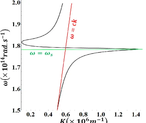
Figure 1.9: Dispersion relation of surface phonon-polaritons at a SiC-Vacuum interface…..25 Figure 2.1: Variation of the RHTC between two semi-infinite Al parallel planes, for the local
model case………..………...…...…...…...…....…...….…...36
Figure 2.2: Variation of the RHTC between two semi-infinite Al parallel planes, for the
Lindhard−Mermin nonlocal model case………..……...…...…...…...…...…….…….41
Figure 2.3: Variation of the RHTC between two semi-infinite Al parallel planes, for the local
and the nonlocal model cases…………...…...…...…...…...…...…………..……...……...41
Figure 2.4: Plot of the transmission coefficient of the p-polarized EM evanescent waves in
the plane (,K) for the local case and the nonlocal case of Lindhard−Mermin model at a
separation distance 𝑑 = 10−12𝑚.……….…..……..……42
Figure 3.1: The dispersion relation of surface optical phonons of semi-infinite ionic crystals
as given by Kliewer and Fuchs………...……….……...48
Figure 3.2: Variation of the RHTC between two semi-infinite 6H-SiC parallel planes, for the
suggested nonlocal model case………...…...…...…...…...…...…...52
Figure 3.3: Variation of the total RHTC between two semi-infinite 6H-SiC parallel planes,
Figure 3.4: Variation of 𝐼𝑚(𝑟3𝑚𝑃 ) as a function of 𝐾 𝑘⁄ for 𝜔 = 𝜔0 𝑇𝑂 for the local model
case and the suggested nonlocal model case.………..……….54
Figure 3.5: Plot of the transmission coefficient, for the local case and the suggested nonlocal
case ……….………...…...…..………...55
Figure 3.6: Variation of the transmission coefficient for 𝜔 = 𝜔𝑇𝑂, for the suggested nonlocal case………...…...…………...56
Figure 3.7: Variation of the RHTC between two semi-infinite 6H- SiC parallel planes, for the
suggested nonlocal model case………...………...…...…...…...…...…...…...…60
Figure 3.8: Variation of the total RHTC between two semi-infinite 6H-SiC parallel planes,
for the local and the suggested nonlocal model cases………...…...…...…...…...….…...60
Figure 3.9: Variation of the total RHTC between two semi-infinite 6H-SiC parallel planes of
average temperature T=300K, for the first and the second suggested nonlocal models………...…...…...…...…...…...…...…...…………...…....………...63
Figure 3.10: Plot of the transmission coefficient, for the local case and the suggested nonlocal
case………..…………...…...…...………..…...…64
Figure 3.11: Variation of the transmission coefficient for 𝜔 = 𝜔𝑇𝑂, for the suggested nonlocal model………...…...…...…...…...…...….………...64
Figure 3.12: Plot of the transmission coefficient for the suggested nonlocal model by
considering d=0 and 𝐾 = 𝑛𝑞𝐵………...…...…..…………...……..…65
Figure 3.13: Variation of the RHTC between two semi-infinite 6H-SiC parallel planes, for
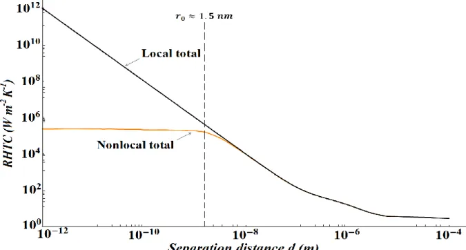
the suggested nonlocal model case when 𝑙 = 𝑟0…………..…...…...…...…...…...…...…69
Figure 3.14: Variation of the total RHTC between two semi-infinite 6H-SiC parallel planes,
for the local case and the suggested nonlocal model case when 𝑙 = 𝑟0………...….…………69
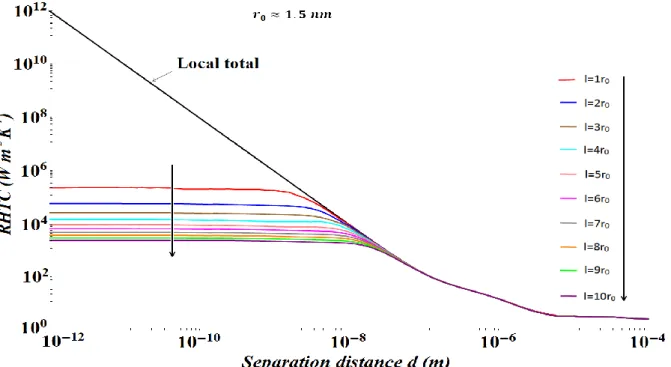
Figure 3.15: Variation of the total RHTC between two semi-infinite 6H-SiC parallel planes,
for the local case and the suggested nonlocal model case when 𝑙 =
(1,2, … 10)𝑟0.……...…...…...…...…...…...…...…...……...…...…...…...…...….……70
Figure 3.16: Plot of the function 𝑓(𝜔, 𝐾) for the local case (l=0) and the suggested nonlocal
cases (𝑙 = 1𝑟0, 3𝑟0, 6𝑟0, 8𝑟0, 10𝑟0)……...…...…...…...…...…...…...…...…...…...…..……....73
Figure 3.17: Variation of the saturation value of the RHTC between two semi-infinite parallel
6H-SiC planes as function of the coherence parameter l. …...…...…...…...…...…...…...…...74
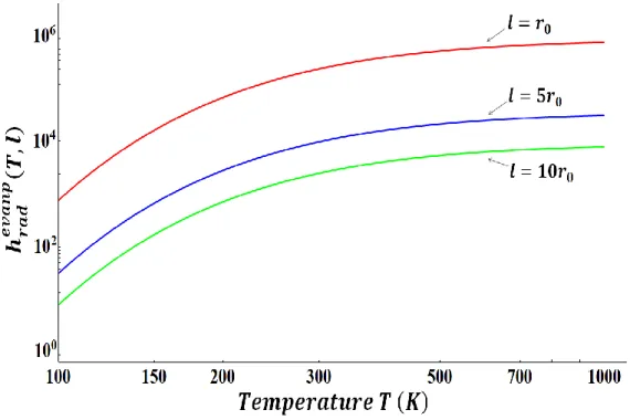
Figure 3.18: Variation of ℎ𝑟𝑎𝑑𝑒𝑣𝑎𝑛 𝑝(𝑇, 𝑙) as function of the average temperature T for the cases
Figure 4.1: A schematic diagram showing the incidence of an EM wave on the interface
separating the local medium (vacuum) from the local dielectric medium, and the nonlocal dielectric medium……...…...….………...………..……....82
Figure 4.2: A schematic diagram showing that an excitation at a point r’ produces a response
at a point r………...………..…....85
Figure 4.3: Variation of the RHTC between two semi-infinite 6H-SiC parallel planes of
average temperature T=300K, for the nonlocal model of Rimbey−Mahan ABC…...91
Figure 4.4: Variation of the RHTC between two semi-infinite 6H-SiC parallel planes of
average temperature T=300K, for the nonlocal model of Agarwal ABC..………...………....92
Figure 4.5: Variation of the RHTC between two semi-infinite 6H-SiC parallel planes of
average temperature T=300K, for the nonlocal model of Ting ABC. ……….…92
Figure 4.6: Variation of the RHTC between two semi-infinite 6H-SiC parallel planes of
average temperature T=300K, for the nonlocal model of Kliewer−Fuchs ABC....…...…...93
Figure 4.7: Variation of the RHTC between two semi-infinite 6H-SiC parallel planes of average temperature T=300K, for the nonlocal model of Pekar ABC..…...…...…...…...…...…...…..…….93
Figure 4.8: Variation of the total RHTC between two semi-infinite 6H-SiC parallel planes for the nonlocal model, with the five different sets of the ABC...…...…...…...…...…...…...…..94
Figure 4.9: Variation of the total RHTC between two semi-infinite 6H-SiC parallel planes,
for the nonlocal model with the five different sets of the ABC, in comparison with the local model………...……...…...…...…...…...…...…...…...…...…...…...…....…...….………....….95
Figure 4.10: Plot of the real part and the imaginary part of the nonlocal dielectric permittivity
function 𝜀(𝜔, 𝐾) in the plane (𝜔, 𝐾)…...…...…...…...………..…..…97
Figure 4.11: Variation of the bump in the curve of the contribution of the p-polarized
evanescent EM waves to the RHTC, as the value of 𝜔𝑝 changes for the nonlocal model of Kliewer−Fuchs ABC…...…...…...…...…...…...…...…...…...…...…...…...…...…….…...…97
Figure 4.12: Variation of the bump in the curve of the contribution of the p-polarized
evanescent EM waves to the RHTC, as the value of 𝜔𝑝 changes for the nonlocal model of Ting ABC…...…...…...…...…...…...…...…...…...…...…...…...…...…...…...…...….……...…...98
Figure 4.13: Variation of the bump in the curve of the contribution of the p-polarized
evanescent EM waves to the RHTC, as the value of the diffusion parameter D changes for the nonlocal model of Kliewer−Fuchs ABC....…...…...…...…...…...…...…...…...…...…...….98
Figure 4.14: Variation of the bump in the curve of the contribution of the p-polarized
evanescent EM waves to the RHTC, as the value of the diffusion parameter D changes for the nonlocal model of Ting ABC…...…...…...…...…...…...…...…...…...…...…...99
Figure 4.15: Variation of the bump in the curve of the contribution of the p-polarized
evanescent EM waves to the RHTC, as the value of the losses parameter ν change for the nonlocal model of Kliewer−Fuchs ABC....…...…...…...…...…...…...…...…...…...…...…...99
Figure 4.16: Variation of the bump in the graph of the contribution of the p-polarized
evanescent EM waves to the RHTC, as the value of the losses parameter ν change for the nonlocal model of Ting ABC…...…...…...…...…...…...…...…...…...…...…...…...…...….100
Figure 4.17: Plot of the transmission coefficient for the local model and the nonlocal model
of Rimbey−Mahan ABC at different separation distances 𝑑…...…...…...…...…...…...…....103
Figure 4.18: Plot of the transmission coefficient for the local model and the nonlocal model
of Agarwal ABC at different separation distances 𝑑……...…...…...…...…...…...104
Figure 4.19: Plot of the transmission coefficient for the local model and the nonlocal model
of Ting ABC at different separation distances 𝑑…..……...…...…...…...…...…..……...105
Figure 4.20: Plot of the transmission coefficient for the local model and the nonlocal model
of Kliewer−Fuchs ABC at different separation distances 𝑑……...…...…...…...…...…...106
Figure 4.21: Plot of the transmission coefficient for the local model and the nonlocal model
of Pekar ABC at different separation distances 𝑑………...…...…...…...…...…...…...…...107
Figure 4.22: Plots of the spectral energy flux and the spectral EM energy density for the
nonlocal model of Rimbey−Mahan ABC at different distances d and average temperature
T=300K…...…...…...…...…...…...…...……...…...…...…...…...…...…...………....…...109
Figure 4.23: Plots of the spectral energy flux and the spectral EM energy density for the
nonlocal case of Agarwal ABC at different distances d of average temperature T=300K….110
Figure 4.24: Plots of the spectral energy flux and the spectral EM energy density for the
nonlocal case of Ting ABC at different distances d and average temperature T=300K…....111
Figure 4.25: Plots of the spectral energy flux and the spectral EM energy density for the
nonlocal model of Kliewer−Fuchs ABC at different distances d and average temperature
T=300K………...…...…...…...…...…...…...……...………..……..112
Figure 4.26: Plots of the spectral energy flux and the spectral EM energy density for the
nonlocal model of Pekar ABC at different distances d and average temperature T=300K....113
Figure 4.27: Plots of the spectral energy flux and the spectral EM energy density, for
Figure 4.28: Plots of the spectral energy flux and the spectral EM energy density, for
different values of the parameter D for nonlocal model of Rimbey−Mahan ABC …….…...114
Figure 4.29: Plots of the spectral energy flux and the spectral EM energy density, for
different values of the parameter D for the nonlocal model of Pekar ABC………....…115 Figure 4.30: Plots of the spectral energy flux and the spectral EM energy density, for different values of the parameter D for the nonlocal model of Ting ABC……….……115
Figure 4.31: Plots of the spectral energy flux and the spectral EM energy density, for
different values of the parameter D for the nonlocal model of Agarwal et al ABC…..…….116
Figure 5.1: Resistivity of Si at T=300K as a function of acceptor and donor concentration.123 Figure 5.2: Variation of the RHTC between two semi-infinite n-doped Si parallel planes of
doping concentration 𝑁 = 1019𝑐𝑚−3 for the local model………...……..123
Figure 5.3: Variation of the RHTC between two semi-infinite n-doped Si parallel planes of
doping concentration 𝑁 = 1020𝑐𝑚−3, for the local model case………124
Figure 5.4: Variation of the RHTC between two semi-infinite n-doped Si parallel planes of
doping concentration 𝑁 = 1021𝑐𝑚−3, for the local model case………....124
Figure 5.5: Variation of the total RHTC between two semi-infinite n-doped Si parallel planes
of doping concentration 𝑁 = 1019cm−3, 1020cm−3and 1021cm−3, for the local model case………...………...125
Figure 5.6: Variation of 𝛿𝐺(𝑇, 𝑁) as function of the average temperature T for the three
different doping concentrations considered in the calculation of the RHTC between the n-doped Si semi-infinite parallel planes………...……...…....127
Figure 5.7: Variation of 𝛿𝐺(𝑇, 𝑁) as function of the doping concentration for different
average temperatures T………...127
Figure 5.8: Variation of the RHTC between two semi-infinite n-doped Si parallel planes of
doping concentration 𝑁 = 1019cm−3, for the nonlocal model case……...………...131
Figure 5.9: Variation of the RHTC between two semi-infinite n-doped Si parallel planes of
doping concentration 𝑁 = 1020cm−3, for the nonlocal model case……….…...…..131
Figure 5.10: Variation of the RHTC between two semi-infinite n-doped Si parallel planes of
doping concentration 𝑁 = 1021cm−3, for the nonlocal model case…………...…………...132
Figure 5.11: Variation of the total RHTC between two semi-infinite n-doped Si parallel
planes of doping concentration 𝑁 = 1019cm−3, 1020cm−3and 1021cm−3, for the nonlocal model case………...132
Figure 5.12: Variation of the total RHTC between two semi-infinite n-doped Si parallel
planes of doping level 𝑁 = 1019𝑐𝑚−3, 1020𝑐𝑚−3and 1021𝑐𝑚−3, for the local and the nonlocal model cases……….……….……133
Figure 5.13: Variation of the saturation value of the RHTC graph as the doping concentration
varies between 1019 𝑐𝑚−3 and 1021 𝑐𝑚−3 for the nonlocal model case where the average temperature of the system is considered T=300K………...134
Figure 5.14: Plot of the transmission for the local case and the nonlocal case for the doping
level 𝑁 = 1019 𝑐𝑚−3 and at different separation distances d………...…..135
Figure 5.15: Plot of the transmission coefficient for the local model and the nonlocal model
for the doping level 𝑁 = 1020 𝑐𝑚−3 and at different separation distances 𝑑………....136
Figure 5.16: Plot of the transmission coefficient for the local model and the nonlocal model
for the doping level 𝑁 = 1021 𝑐𝑚−3 and at different separation distances 𝑑……...…137
Figure 5.17: Variation of the spectral radiative heat transfer flux of the p-polarized EM evanescent waves as varies for different doping concentrations N in the nonlocal model
case and for a separation distance 𝑑 = 10−12𝑚………..…...138
Figure A.1: Geometry of the system considered (2−interfaces)………...147 Figure A.2: Presentation of the different vectors of the EM waves of s and p polarizations,
introduced in the formalism of Sipe 1987 for the 2−interfaces system………...…...148
Figure B.1: Geometry if the system considered (1−interface)………...……...….158 Figure B.2: Presentation of the different vectors introduced in the formalism of Sipe 1987 for
List of Abbreviations
6H-SiC 6H-type Silicon Carbide
ABC Additional boundary conditions
DRHF Density of the radiative heat flux EM Electromagnetic
FFRHT Far-field radiative heat transfer FDT Fluctuation-dissipation theorem FBZ First Brillouin zone
IR Infrared
LDOS Local density of states
MIT Massachusetts Institute of Technology
n-Si n-doped Silicon
NFRHT Near-field radiative heat transfer
NSOM/SNOM Near-field Scanning Optical Microscopy () PINEM Photon-induced near-field electron microscopy RHT Radiative heat transfer
RHF Radiative heat flux
RHTC Radiative heat transfer coefficient
RPA Random phase approximation
STM Scanning Tunneling Microscopy
STM Scanning Tunneling Microscope SFM Scanning Force Microscopy
SSP Surface scattering parameters
List of symbols
Greek Letters
Normalized damping factor 𝛱(𝒓, 𝜔) Poynting vector ( 𝐽. 𝑠−1. 𝑚−2) ℙ Excitation polarization (𝐶 𝑚⁄ 2)
Exchanged radiative heat flux (𝑊. 𝑚−2) 𝛷 Spectral flux energy density ( 𝐽. 𝑚−2. 𝑟𝑎𝑑−1) 𝛺 Normalized frequency factor
𝛾 Normal wavevector component 𝑚−1 𝛿𝑘,𝑙 Kronecker symbol
𝛿 Dirac delta function
δ Skin depth (𝑚) 𝜖 Emissivity
𝜀 Dielectric permittivity function 𝜀∞ Infinite frequency permittivity
𝜀0 Dielectric permittivity of vacuum (𝐹. 𝑚−1) Ѳ Mean energy of the harmonic oscillator in ( 𝐽) κ Thermal conductivity (𝑊. 𝑚−2. 𝐾−1)
λ Wavelength of thermal radiation (𝑚)
𝑚𝑎𝑥 Wien’s wavelength in (𝑚) 𝜇0 Vacuum permeability (𝐻. 𝑚−1)
ν Frequency of thermal radiation (𝐻𝑧) 𝜈 Damping factor (𝑟𝑎𝑑. 𝑠−1)
𝝆 Polarization at an interface (𝐶 𝑚⁄ 2) 𝜌 Electric resistivity (𝛺 ⋅ 𝑐𝑚)
𝜎 Stefan−Boltzmann constant in (𝑊. 𝑚−2. 𝐾−4) 𝜏 Relaxation time (𝑠)
𝜏 Transmission coefficient of the electromagnetic wave 𝜐𝐹 Fermi velocity (𝑚. 𝑠−1)
̃ Susceptibility tensor
𝜔 Angular frequency (𝑟𝑎𝑑. 𝑠−1) 𝜔𝑝 Plasma frequency (𝑟𝑎𝑑. 𝑠−1)
𝜔𝐿 Optical longitudinal angular frequency (𝑟𝑎𝑑. 𝑠−1) 𝜔𝑇 Optical transverse angular frequency (𝑟𝑎𝑑. 𝑠−1)
𝜔𝑠𝑝 Surface plasmon-polaritons excitation frequency (𝑟𝑎𝑑. 𝑠−1)
Latin letters
A Adjusted constant B Adjusted constant
𝐶1 First radiation constant (𝑊. 𝜇𝑚4/𝑚2) 𝐶2 Second radiation constant (𝜇𝑚. 𝐾) 𝐶3 Third radiation constant (𝜇𝑚. 𝐾)
D Constant related to a diffusion phenomenon of the carriers (𝑚2. 𝑠−2)
𝑫 Displacement vector (𝐴. 𝑚−1) 𝑬 Electric field (𝑉. 𝑚−1)
𝐸λ,𝑏 Spectral emissive power of a blackbody (W/m².μm) 𝑮
⃡ Green tensor
𝐽 Radiative heat flux between two real opaque bodies (𝑊. 𝑚−2) 𝐽𝑏𝑏 Radiative heat flux between two blackbodies (𝑊. 𝑚−2) 𝐾 Parallel wavevector component (𝑚−1)
N Doping concentration (𝑐𝑚−3)
𝑁𝑐 Effective density of states in the conduction band (𝑐𝑚−3)
T Temperature (K)
𝑈 Surface scattering parameters
Z Surface impedance (𝑚. 𝑠−1) c Speed of light in vacuum (𝑚. 𝑠−1) d Distance (𝑚)
dc Critical distance (𝑚) 𝑒 Electron charge (𝐶)
𝑔0 Quantum of the thermal conductance (𝐽. 𝑠−1. 𝐾−1)
h Planck’s constant in (𝐽. 𝑠)
ћ Reduced Planck constant (or Dirac constant) (𝐽. 𝑠)
ℎ0 Derivative of the black body specific intensity of radiation with respect to temperature (Planck's law) (𝐽. 𝑠−1. 𝑚−2. 𝐾−1)
ℎ𝑟𝑎𝑑 Radiative heat transfer coefficient (𝑊. 𝑚−2. 𝐾−1) 𝑗(𝒓, 𝜔) Current density at point r in (𝐴. 𝑚−2)
𝑘𝐵 Boltzmann constant in (𝐽. 𝐾−1)
𝒌 Total wavevector of the EM wave in (𝑚−1) 𝑘0 Total wavevector in vacuum (𝑚−1)
𝑘𝐹 Fermi wavevector (𝑚−1)
l Coherence length of the thermal EM field (𝑚)
𝑙𝑇𝐹 Thomas−Fermi length (𝑚) 𝑚𝑒 Electron mass (Kg)
𝑚ℎ Hole mass (Kg)
𝑚∗ Electron effective mass (Kg)
q Tangential wavevector component (𝑚−1)
𝑟 Reflection coefficient of the EM wave 𝑟0 Lattice constant (𝑚)
1
Introduction
This thesis is devoted to the study of the influence of the nonlocal effects on the near-field radiative heat transfer. Conducting this study for a system consisting of two semi-infinite parallel solid dielectric planes, we present the consequences of accounting for the nonlocal effects in the dielectric permittivity model on the exchanged radiative heat flux. One of the major consequences is the saturation of the radiative heat transfer coefficient, which replaces the non-physical divergence obtained upon using a local model of the dielectric permittivity.
The originality of this work consists in three main points. The first point is suggesting four different nonlocal models of the dielectric permittivity for dielectrics, which take into consideration the spatial dispersion and the nonlocal effects. Throughout the past few decades, most of the theoretical studies of the radiative heat transfer between two objects involved local models of the dielectric permittivity and nonlocal effects were not included. Obtaining some results that could not be considered physical, such as the infinity diverging radiative heat transfer coefficient as the inter-planar distance decreases, the authors conducting these studies suggested that considering a nonlocal model of the dielectric permittivity could be the solution. As far as we know, the nonlocal models of the dielectric permittivity that were suggested after that were complicated as to be handled analytically and numerically. For this reason, the second point that constitutes the originality of our work is the simplicity of our suggested nonlocal models of the dielectric permittivity. We will show throughout the different aspects of our work the simple mathematical and analytical treatment of these models, as well as the clarity of the different physical notions portrayed in their expressions. The third point would definitely relate to the results; obtaining saturation of the radiative heat transfer coefficient as the inter-planar distance decreases between the dielectric planes constitutes one main original point. Our suggested nonlocal dielectric models lead to replacing the nonphysical divergence with a finite saturation, backed up with the analytical calculations, the numerical simulations, the physical interpretations and the supporting references.
2
- Chapter 1 presents an introduction to the different aspects of our work. Starting with the description of the thermal energy and the radiative heat transfer, we demonstrate the characteristics of the far-field radiative heat transfer and the near-field radiative heat transfer, along with their physical differences. Showing the importance of the near-field radiative heat transfer in the different technological domains, and explaining the physical phenomena dominating this transfer, we highlight the physical bases needed to conduct our work. We then present the detailed near-field radiative heat transfer study for a system of two semi-infinite parallel 6H-SiC planes using a local model of the dielectric permittivity. We show how the radiative heat transfer diverges as the inter-planar distance decreases.
- Chapter 2 is dedicated to studying the near-field radiative heat transfer for a system of two semi-infinite parallel metallic planes using a local model of the dielectric permittivity. We then proceed by repeating the complete work of Chapuis et al. to perform the same study as the previous section, using a nonlocal model of the dielectric permittivity.
- Chapter 3 includes the detailed study of three of our suggested nonlocal models of the dielectric permittivity for dielectrics. Considering the same system as in the local study in chapter 1, we present each model along with the validity conditions and the related results. We also compare between the different results and features. We show that saturation of the radiative heat transfer coefficient is attained in the three models. - Chapter 4 presents the fourth suggested nonlocal model of the dielectric permittivity
for dielectrics. It is based on the macroscopic theory of Halevi and Fuchs. This theory considers spatial dispersion and electromagnetic excitation at the surface of the dielectrics. We will show that the latter of these assumptions necessitates some additional boundary conditions. We will consider five different sets of these ABC and use them in the study of the near-field radiative heat transfer for the same 6H-SiC system. Saturation and other different interesting physical features are obtained, and consequently explained throughout the chapter.
- Chapter 5 is devoted to studying the near-field radiative heat transfer for a system of two n-doped silicon planes. We start with preforming this study using a local model of the dielectric permittivity. The nonphysical divergence is obtained, and for this reason we repeat in the second section the same study using a nonlocal model of the dielectric permittivity. The model used is the same one considered in chapter 2 for the metallic planes case. We will show that the saturation of the radiative heat transfer coefficient
3
is obtained. Different physical features are presented and interpreted with respect to the variation of the doping concentration, and the average temperature of the system. The last part is dedicated to the conclusions and the future perspectives; followed by the appendices A, B, C, D and E demonstrating in details the necessary derivations mentioned throughout the report.
4
Chapter 1
1. Introduction to Radiative Heat Transfer
Introduction
Thermal radiation is a well-known physical phenomenon that was described since the beginning of the last century by Planck [1] and Einstein [2,3]. It is defined as the radiant energy emitted by a medium and that is due solely to the temperature of this medium, i.e. it is the temperature of the medium that governs the emission of thermal radiation. We refer by thermal radiation or radiative heat transfer (RHT) to the phenomenon describing the heat transfer due to the propagation of electromagnetic (EM) waves. Unlike the other two mechanisms of energy transfer, conduction and convection, RHT requires no intervening medium to propagate which makes it of great importance for many applications in different fields [4−6]. Very often, the RHT from cooler bodies can be neglected in comparison with convection and conduction; but heat transfer processes that occur at high temperature, or with conduction or convection suppressed by evacuated insulations (different kinds of insulations evacuated from gas), usually involve a significant fraction of radiation. RHT plays an important role in the transfer of heat in the furnaces and the combustion chambers; as well as in the energy emission of nuclear explosions. In general, heat transfer considerations are important in almost all the domains of technology; heat transfer involves a great variety of physical phenomena and engineering systems [7].
In the EM radiation spectrum, the thermal radiation at usual temperatures lies in the intermediate portion extending from 0.1 𝜇𝑚 to 100 𝜇𝑚 including a part of the ultraviolet (UV) range, all the visible range and all the infrared (IR) range; see Fig. 1.1 [4]. Thermal radiation exhibits the same wavelike properties as light or radio waves where each quantum of radiant energy has a wavelength “λ” and a frequency “ν” associated with it.
Any material of finite temperature emits and absorbs continuously heat radiation in all directions due to the molecular and atomic motions associated with its internal energy.
5
Figure 1.1: The electromagnetic spectrum [4].
The strength of the emission depends on the temperature and all real bodies emit and absorb heat less than a blackbody at the same temperature. The blackbody is considered as the standard against which the behavior of all real radiating materials is estimated and compared; and its properties are well-defined in theory. In general, it is defined as a surface or volume that absorbs all incident radiation at every wavelength and from any direction, and it is considered also as the best possible emitter of radiation, at every wavelength and in every direction. As a consequence, any real material will reflect some of the incident radiation and therefore it will absorb energy less than that absorbed by the ideal blackbody; similarly, a real body will emit energy less than emitted by the ideal blackbody [4−6].
Since the end of the nineteenth century, scientists had tried for many years to predict the spectrum of the blackbody emission, starting from Wilhelm Wien 1896 [8] who used thermodynamic arguments along with some experimental data to propose a spectral distribution of the blackbody emissive power; a large part of this spectrum was accurately correct. Lord Rayleigh and Sir Jeans derived a spectral distribution of the blackbody emissive power based on the assumption that the equipartition theorem of energy is valid [7,9]; they expressed the energy density as the product of the number of standing waves, which were considered as oscillators, and the average energy of an oscillator. They found the average energy of an oscillator of temperature T to be independent of the frequency and equal to 𝑘𝐵𝑇, where 𝑘𝐵 = 1.380648 × 10⁻²³𝐽. 𝐾−1 is Boltzmann constant. This Rayleigh−Jeans law agreed well with the experimental observations for small frequencies, but for large
6
frequencies, i.e. for the ultraviolet range, this law gave results that were very different from the experimental results. This error in the values of Rayleigh−Jeans law is known as the ultraviolet catastrophe.
In 1900, based on his work on quantum statistics, Planck [1] published the correct spectral emissive power spectrum of a blackbody where he assumed that a molecule can emit photons only at distinct energy levels. The spectral emissive power (in W/m².μm) is given by the following equation [1, 4−6]:
𝐸λ,𝑏(, 𝑇) = 𝐶1
𝜆5[𝑒𝐶2⁄𝑇− 1] (1.1)
is the wavelength, T is the absolute temperature, 𝐶1 = 2𝜋ℎ𝑐2 = 3.742 × 10⁸ 𝑊. 𝜇𝑚4/𝑚2
and 𝐶2 = ℎ𝑐 𝑘⁄ 𝐵 = 1.439 × 10⁴𝜇𝑚. 𝐾 are the first and the second radiation constants, respectively. ℎ = 6.626069 × 10⁻³⁴𝐽. 𝑠 is Planck’s constant and 𝑐 = 2.998 × 10⁸𝑚. 𝑠−1 is the speed of light in vacuum.
Wien’s displacement law [8] published in 1891 independently and well before Planck’s law allows calculating at any temperature T, the wavelength 𝑚𝑎𝑥 at which the emitted power of the blackbody is maximal. This law is given by the following equation [4,5,6,10,11]:
𝑚𝑎𝑥 = 𝐶3
𝑇 (1.2)
where 𝐶3 = 2898 𝜇𝑚. 𝐾 is the third radiation constant. In Fig. 1.2 we present the emissive power spectrum obtained from Planck’s equation Eq. (1) along with the locus of Wien’s equation Eq. [2], where we observe that the power increases and 𝑚𝑎𝑥 shifts to smaller values as the temperature increases [4].
Followed by the work of Einstein [2,3] in 1907 and 1916 that generalized Plank’s law and gave clear definitions, the notions associated to thermal radiation were well presented and thus well-understood since then.
One of the typical studies of the RHT phenomenon is the study of the energy transfer exchanged between two bodies of different temperatures. When the bodies are separated by a vacuum gap of width d, the heat flux exchanged between them is only due to RHT.
Classical RHT between two semi-infinite bodies does not depend on the distance between them, but on the optical properties of the bodies. More recently, it has been shown that the radiative heat flux (RHF) transferred between two bodies increases and reaches values of several orders of magnitude larger than the classical RHT as the gap distance decreases.
7
Figure 1.2: The spectral emissive blackbody power as given by Planck’s law [4]. The straight
line connecting the peaks of the graphs corresponds to the locus of the wavelength given by Wien’s displacement law.
This happens when the typical gap distance becomes much smaller than the thermal wavelength 𝑚𝑎𝑥; i.e. this typical wavelength separates the far-field range where the classical RHT is valid, from the near-field range where the wave effects come into play [12,13].
In the past years the importance of studying and evaluating the heat transfer in the near-field has significantly increased due to particular technological challenges [14]. The recent development of micro and nanotechnologies posed new fundamental and technological problems as the dissipated power per unit volume in these devices is becoming increasingly important due to the reduced size and the increased performance of such systems. Nevertheless, the evacuation of this power is also increasingly difficult leading to undesired consequences as the heating of many electronic or optoelectronic components affects their performance and their life span [15]. The need to solve these problems or at least to limit their consequences had led to the importance of measuring and controlling the temperature and the radiated energy at micro and nano-scales.
We start by recalling the far-field radiative heat transfer (FFRHT) using the classical theory of heat radiation. For a system consisting of two bodies of temperatures 𝑇1and 𝑇2 separated by a vacuum gap of width 𝑑 ≫ 𝑚𝑎𝑥, the heat radiation exchanged between them is due to the EM waves travelling through the vacuum gap. When the two bodies are considered
8
as perfect absorbers, i.e. when they act as blackbodies [1, 16], the RHT flux between them is maximal and by Stefan−Boltzmann law it is given as follows [17]:
𝐽𝑏𝑏 = 𝜎(𝑇14− 𝑇
24) (1.3)
where 𝜎 = 𝜋2𝑘𝐵4⁄60ћ3𝑐2 = 5.67 × 10⁻⁸𝑊𝑚−2𝐾−4 is the Stefan−Boltzmann constant and ћ = 1.054571 × 10⁻³⁴𝐽. 𝑠 is the reduced Planck constant (or Dirac constant). We notice from Eq. (1.3) that the RHT flux density is independent of the gap distance d between the bodies and it depends on the difference of their absolute temperatures each raised to the fourth power. For real opaque bodies the Stefan−Boltzmann law is modified and the RHT flux density is given as follows:
𝐽 = 𝜎𝜖12(𝑇14− 𝑇24) (1.4)
where 𝜖12 is effective emissivity that depends on the emissivities of the bodies 𝜖1and 𝜖2 and a corrective factor called the view factor 𝐹12. The emissivity of a body is defined as its ability to emit radiation compared to the ideal emission of a blackbody at the same temperature. This implies that for real bodies, the values acquired by 𝜀 are given by: 0 < 𝜖 < 1. For the special case where the opaque bodies are two semi-infinite parallel plates, Eq. (1.4) reduces to the following form:
𝐽 = 𝜎 𝜖1𝜖2
1 − 𝜌1𝜌2(𝑇14− 𝑇24) (1.5)
where 𝜌 is the reflectivity of the body defined as the fraction of the incident radiative energy reflected by this body.
For the near−field radiative heat transfer (NFRHT), the classical theory does not apply as in this case the gap distance d considered is of the order of or smaller than Wien’s wavelength
𝑚𝑎𝑥. It had been shown by many studies that the near-field radiation allows heat to propagate across a small vacuum gap at rates several orders of magnitude higher than that of the far-field blackbody radiation [12,13,17−23].
Cravalho et al. [12] and Polder and Van Hove [13] presented the pioneering work of studying the radiative heat transfer in the near-field by showing the RHF significant increase when the bodies are approached, until this flux reaches values of many orders higher than that between two blackbodies [1,24]. This increase in the NFRHF was interpreted to be due to different complex physical wave phenomena [9,13,18−21,24,25] taking place at small
9
distances. The phenomena playing the most important role are the interference effects in the waves between the two surfaces and the tunneling evanescent waves.
Evanescent waves are EM waves that dominate the RHT at small distances. They tunnel between two surfaces, and their contribution increases as the separation distance decreases, and they decay exponentially as the distance increases [12,13,21−26]. In general, the first recognition of the existence of evanescent electromagnetic waves was probably the analysis of the skin depth effect at metallic surfaces [17−31]. Years later, following the work of Cravalho et al. [12] and Polder and VanHove [13], a lot of theoretical and experimental research had been devoted to the study of NFRHT between bodies of different materials and different geometrical configurations as this heat transfer mechanism exhibits complex wave phenomena [12,13,21,24−28]. As it is shown in Fig. 1.3 [30], when two surfaces are approached to each other, some of the photons tunnel between the two mediums; new channels of transfer are open corresponding to modes of large wavevectors parallel to the surface by which heat transfer is enhanced.
Figure 1.3: Evanescent waves decay exponentially away from the surface and play
important role when two planes approach each other as they tunnel between the surfaces of the two planes and contribute effectively to the heat transfer at small
separation distances [32].
The science of the EM evanescent waves had drawn a lot of attention because of the different promising technological enhancements that could be achieved using the properties of these waves. As an example, some researchers at the Massachusetts Institute of Technology
10
(MIT) had proposed a plan for wireless power transfer based on the idea that evanescent wave coupling describes how electromagnetic energy can be sent from one device to another by the way of a decaying electromagnetic field. They were driven by their interest in using wireless technology to charge or power devices which led them to greater understanding of the principles of wireless evanescent coupling. They demonstrated a way to wirelessly send and receive power from a local transmitter to a receiver that is in the vicinity of the device, and in 2007 they showed how a 60 Watt light bulb could be powered up from a distance of 2 meters. They used a technology termed “WiTricity” as an abbreviation of “wireless electricity” to describe this phenomenon of evanescent wave coupling at resonance [33].
The practical exploitations of the evanescent waves, their decaying characteristic and the exponential nature of their wavefunction were undeveloped for a long time until the emergence of local probe-based methods (Scanning Tunneling Microscopy (STM), Scanning Force Microscopy (SFM), and Near-field Scanning Optical Microscopy (NSOM/SNOM)) in the early 1980s with the beginning of the actual investigation of the near-field physics [34−37]. This was followed by many studies at subnanoscale resolution that were achieved due to the evanescent waves effects [38]. Almost two decades later, the research team of A. Zewail exploited the characteristics of the evanescent waves to invent a new type of imaging technique that combines the best qualities from electron microscopy and light microscopy; they called it photon−induced near−field electron microscopy (PINEM) [39]. Nevertheless, superluminal effects of evanescent waves have been revealed in photonic tunneling experiments in both the optical and the microwave domains [39−47].
On the other hand, and due to its different characteristics, NFRHT became crucial in the development of potential applications in numerous technologies such as solar cells and thermophotovoltaic sources [26,49−51], nanolithography [51,52] and sub-wavelength light sources [53].
A lot of theoretical studies were carried out for systems consisting of two semi-infinite plane-parallel solid surfaces. These studies aimed to calculate the NFRHT between the two planes using a local dielectric permittivity function, as the optical response of the material was considered local i.e. 𝜀 = 𝜀(𝜔), where 𝜔 is the angular frequency of the EM wave. These studies have shown different behaviors according to the type of the considered material.
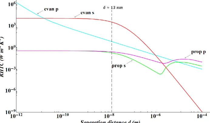
For dielectrics, the NFRHT follows a 1 𝑑⁄ law starting at distances as large as few 2 hundreds of nm [13,21,24,26].
11
For metals, it was shown that the transfer seems to saturate at distances below the material skin depth and then diverges with a 1 𝑑⁄ law at extremely small separation distance d below 2 1 nm [28,54,55]. We will present in chapter 2 our study of the RHT between two semi-infinite parallel metallic planes where we demonstrate and discuss these results.
Following these theoretical predictions, some experimental studies were carried out to study the RHT between different bodies as the separation distance decreases [55−59]. The obtained results confirmed the enhancement of the RHTF in the nanometer regime due to the tunneling of evanescent waves at the surfaces. Nevertheless, some of the experimental studies have roughly confirmed the 1 𝑑⁄ law mostly at micrometric distances [58]. In the following 2 sections (and chapters) we will present these studies, their results and their discussions in details.
The 1 𝑑⁄ diverging law as the separation distance d is reduced cannot be followed at 2 extremely small distances as no heat transfer can become infinite. Moreover, the continuous behavior of matter does not exist at the atomic scale so that matter response inevitably changes for high spatial frequency. This leads to the need of a nonlocal description of the matter response as suggested by various authors [21,24,61]. In this case, the dielectric permittivity function will be not only frequency dependent but also wavevector dependent.
This constitutes the main subject of this thesis, as we study the validity of few nonlocal models of the dielectric permittivity in the calculation of the radiative heat transfer coefficient (RHTC) between two semi-infinite parallel dielectric planes. For the case of two metallic planes, Chapuis et al. [54] have studied the Lindhard−Mermin nonlocal dielectric permittivity function model and showed that the NFRHT saturated at distances of the order of the Thomas−Fermi length and also suppressed the 1 𝑑⁄ divergence that occurred at extremely 2 small distances. In chapter 2 we present these results along with their detailed explanation.
In the following sections we will present in details the study of the RHT between two solid semi-infinite parallel planes. We will start by presenting the main ideas that allow treating the RHT in electromagnetism in sections 1.1 and 1.2: the Fluctuation-dissipation theorem, the thermodynamic equilibrium and the correlation equation of the fluctuating currents needed in the derivation of the RHTC equation. In section 1.3 we show our calculations of the RHTC between two 6H-type Silicon Carbide semi-infinite parallel planes as the distance between them approaches zero, using a local model of the dielectric permittivity. Section 1.4 will be devoted to the conclusions of this chapter.
12
1.1 Fluctuation-Dissipation Theorem
In the far-field the emitted electromagnetic field is well described using radiometry theory that is based on the geometrical optics, while in the near-field this theory ceases to be valid as it does not take into consideration the evanescent waves that play an important role in the NFRHT. This leads to the necessity of deriving a formalism that describes well the EM field at small distances. Therefore, one has to use Maxwell equations to calculate the EM field emitted by a body of temperature T. This is the aim of the Fluctuational Electrodynamics formalism, first suggested by Rytov [21, 27,62].
The Fluctuational Electrodynamics states that a body of temperature 𝑇 > 0 𝐾 in local thermo-dynamical equilibrium radiates thermal energy due to the fluctuations of random currents generated by the random thermal motion of the charges of the body. These charges are electrons in metals and ions in polar materials. The properties of these currents are given by the fluctuation-dissipation theorem (FDT) relating the currents correlation function to the medium radiative losses. These currents radiate an EM field related to the currents by the Green’s tensors of the system. This implies that knowing the properties of the random currents and the radiation of a volume element below the interface is essential to determine the statistical properties of the radiated field. Defining the density of the fluctuating current at any point in the medium and substituting it in Maxwell’s equations enable us to treat the thermal radiation in electromagnetism [21].
Formalism
The overall current correlation function is a non-zero average and is given by the FDT. We consider a nonmagnetic material body described from an electromagnetic point of view by its dielectric constant 𝜀(𝜔). We assume that the dielectric permittivity is local, i.e. the polarization at a certain point of the medium is directly proportional to the electric field at this point , and does not directly depend on the field of other points. Moreover, the body is assumed to be in local thermodynamic equilibrium, i.e. at any instant the temperature of any point of the material is T.
Considering these assumptions as basic, we define the two current densities at points r and
r’ situated in the medium by 𝑗(𝒓, 𝜔) and 𝑗(𝒓′, 𝜔′), oscillating at frequencies 𝜔 and 𝜔′ respectively, as shown in Fig.1.4.
13
Figure 1.4: A schematic diagram of the geometry of the system.
The FDT then defines the correlation equation of the currents as follows: 〈𝑗𝑘(𝒓, 𝜔)𝑗𝑙∗(𝒓′, 𝜔′)〉 =
𝜔𝜀0
𝜋 𝐼𝑚(𝜀(𝜔))Ѳ(𝜔, 𝑇)𝛿𝑘,𝑙𝛿(𝒓 − 𝒓′)𝛿(𝜔 − 𝜔′) (1.6)
where 〈… 〉 indicate an ensemble average. 𝑘, 𝑙 = 𝑥, 𝑦, 𝑧 correspond to the different spatial components (in Cartesian coordinates) of the currents. 𝜀0 = 8.85417 × 10⁻¹² 𝐹. 𝑚−1 is the dielectric permittivity of vacuum and 𝐼𝑚(𝜀(𝜔)) is the imaginary part of the material’s dielectric permittivity. 𝛿𝑘,𝑙 is Kronecker symbol and 𝛿 is Dirac delta function. Ѳ(𝜔, 𝑇) = {(ћ𝜔 2⁄ ) + [ћ𝜔 (𝑒⁄ ћ𝜔 𝑘⁄ 𝐵𝑇− 1)]} is the mean energy of the harmonic oscillator of frequency
𝜔 at temperature T and ћ𝜔 2⁄ represents the vacuum energy, called the zero-point energy. The latter term vanishes from the final results in the case of radiative energy transfer [21]. A simple interpretation would be that we suppose that the medium considered is the only source of fluctuating fields. However the fluctuations of vacuum exist in the presence and absence of the medium, and whether the temperature is zero or not. Therefore, we consider that at any instant, the zero-point energy emitted by a volume element is compensated by an absorbed flux coming from the rest of the space, leading to equilibrium [21].
From Eq. (1.4) we deduce that the fluctuating currents are 𝛿-correlated in space (spatial locality of the dielectric constant) and the fluctuation amplitude is directly related to the losses in the system given by the term 𝐼𝑚(𝜀(𝜔)). Furthermore, understanding how the medium radiates EM waves into space is achieved when the dielectric permittivity of the medium is known. Propagation of waves from the sources (currents) to the observation point is given by the knowledge of the Green function depending on the geometry and the optical properties (𝜀(𝜔)).
14
The FDT is considered the starting point for the derivation of the RHTC exchanged between two bodies, as it will be presented in the following section.
1.2 Radiative heat transfer coefficient
In this section we will use the FDT to derive the equation of the RHTC exchanged between two semi-infinite parallel planes of temperatures T1 and T2 [13,17,18,21,23,63−65],
see Fig. 1.5.
The system considered is divided into three media subspaces: the first subspace corresponding to z < 0 is occupied by medium (1) whose properties are described by the dielectric permittivity 𝜀1 and similarly, the second subspace corresponding to z > d is occupied by medium (2) and described by the dielectric permittivity 𝜀2; subspace (3) corresponds to 0 < z
< d and is occupied by vacuum described by the dielectric permittivity 𝜀3. At this stage of our study the nature of the media (metals, dielectrics …) does not affect the derivation and so it will not be specified.
Figure 1.5: Two parallel semi-infinite material planes separated by a vacuum gap of width d.
In the most general sense, constitutive relations in a medium that relate bound charges to the electric field depend on the wave vector and the frequency so that for example 𝑫(𝒌, 𝜔) = 𝜀(𝒌, 𝜔)𝑬(𝒌, 𝜔), where 𝑫(𝒌, 𝜔) is the displacement vector and 𝑬(𝒌, 𝜔) is the electric field. When the EM field varies on a spatial scale larger than the microscopic characteristic lengths of the propagation medium, the medium is referred to as local so that the characteristic quantities of the medium are frequency-dependent only, i.e. 𝑫(𝒓, 𝜔) = 𝜀(𝒓, 𝜔)𝑬(𝒓, 𝜔). When this is not the case, the medium is said to be nonlocal, i.e. the optical properties depend on the
15
wavevector of the EM field [21,24]. In other words, we can say that in the case of nonlocality, the polarization at one point in the nonlocal medium depends not only on the electric field at that point, but also on the electric fields at the surrounding points. To illustrate this condition clearly, for the case of dielectrics for example, a so-called single-oscillator nonlocal model of the dielectric permittivity 𝜀(𝒌, 𝜔) [66] is used (this model is represented in details in chapter 4) where the spatial dispersion, and eventually the nonlocality condition, is presented schematically in Fig. 1.6. We will discuss the nonlocality case in details in the following chapters.
Figure 1.6: A schematic diagram of a dielectric medium when spatial dispersion is neglected
(a) and when spatial dispersion is taken into consideration (b) [66].
1.2.1 Brief recall of the radiometric approach
This approach is based on two main concepts: the geometrical optics and the luminous ray nature of the radiation. The exchanged energy flux originates due to the multiple reflections of the radiation in vacuum at the interfaces of planes 1 and 2. Performing few simple algebraic steps we obtain finally the following expression for the exchanged RHF between the two planes separated by vacuum [21,67]:
1,2 = ∫ cos 𝜃 𝑑 2𝜋 0 ∫ 𝑑𝜔 ∞ 0 𝜖1𝜔′ 𝜖 2𝜔′ 1 − 𝜌1𝜔′ 𝜌 2𝜔′ [𝐿𝜔 0(𝑇 1) − 𝐿0𝜔(𝑇2)] (1.7)
where is the solid angle considered to study the radiation in a direction of angle 𝜃 with respect to the z axis. 𝜖1𝜔′ and 𝜖
16
and (2), respectively. 𝐿0𝜔(𝑇) = ћ𝜔3⁄[4𝜋3𝑐2(𝑒ћ𝜔 𝑘⁄ 𝐵𝑇− 1)] is the monochromatic specific
intensity of radiation of a blackbody of temperature 𝑇 as given by Planck’s law.
For the study of the radiation in the near field, this approach is not valid anymore. Regarding the concept, this approach does not take into account the wave nature of the radiation which leads to neglecting the interference phenomena in the studies. Another important negative point of this approach is the total neglecting of the role of the tunneling evanescent waves between the two interfaces because tunneling is a consequence of the wave behavior of radiation. The role of evanescent waves becomes dominant in the small distance range, and neglecting their role in the near-field leads to huge error in the study of the RHT.
This imposed the importance of having a different approach taking into consideration the different phenomena appearing at small distances, in addition to the tunneling EM evanescent waves. The EM approach presented in the following section solves these problems and accounts for the different near-field properties.
1.2.2 Electromagnetic approach
The emitted radiative flux is given by the Poynting vector
〈𝛱(𝒓, 𝜔)〉 = 4 ×12𝑅𝑒[〈𝑬(𝒓, 𝜔) × 𝑯∗(𝒓, 𝜔)〉] [21, 51,65] , where 𝑬(𝒓, 𝜔) and 𝑯(𝒓, 𝜔) are the electric field and magnetic field Eqs. (6) and (7), respectively [37,53]. The factor “4” comes from the fact that the signals considered here have positive frequencies only, so that the fields are analytic signals [21].
𝑬(𝑟, 𝜔) = 𝑖𝜔𝜇0∫ 𝑮⃡ 𝐸(𝒓, 𝒓′, 𝜔) ∙ 𝒋
𝑓(𝒓′, 𝜔)𝑑3𝒓′ (1.8)
𝑯(𝑟, 𝜔) = ∫ 𝑮⃡ 𝐻(𝒓, 𝒓′, 𝜔) ∙ 𝒋
𝑓(𝒓′, 𝜔)𝑑3𝒓′ (1.9)
r’ corresponds to the “source point” situated in the plane (2) and r is the observation point
situated in plane (2). 𝑮⃡ 𝐸(𝒓, 𝒓′, 𝜔) and 𝑮⃡ 𝐻(𝒓, 𝒓′, 𝜔) are the Green tensors of the medium. The Green function equations are used to link the EM field at the point r to the current density at point r’. Their expressions along with the explanations are given in Appendix A.
It follows that
![Figure 3.1: The dispersion relation of surface optical phonons of semi-infinite ionic crystals as given by Kliewer and Fuchs [5]](https://thumb-eu.123doks.com/thumbv2/123doknet/14501245.719266/67.892.168.735.591.885/figure-dispersion-relation-surface-optical-infinite-crystals-kliewer.webp)