RESEARCH OUTPUTS / RÉSULTATS DE RECHERCHE
Author(s) - Auteur(s) :
Publication date - Date de publication :
Permanent link - Permalien :
Rights / License - Licence de droit d’auteur :
Bibliothèque Universitaire Moretus Plantin
Institutional Repository - Research Portal
Dépôt Institutionnel - Portail de la Recherche
researchportal.unamur.be
University of Namur
Empirical Assessment of Generating Adversarial Configurations for Software Product
Lines
Temple, Paul; Perrouin, Gilles; Acher, Mathieu; Biggio, Battista; Jézéquel, Jean-Marc; Roli,
Fabio
Published in:
Empirical Software Engineering
Publication date:
2020
Document Version
Peer reviewed version
Link to publication
Citation for pulished version (HARVARD):
Temple, P, Perrouin, G, Acher, M, Biggio, B, Jézéquel, J-M & Roli, F 2020, 'Empirical Assessment of Generating Adversarial Configurations for Software Product Lines', Empirical Software Engineering .
General rights
Copyright and moral rights for the publications made accessible in the public portal are retained by the authors and/or other copyright owners and it is a condition of accessing publications that users recognise and abide by the legal requirements associated with these rights. • Users may download and print one copy of any publication from the public portal for the purpose of private study or research. • You may not further distribute the material or use it for any profit-making activity or commercial gain
• You may freely distribute the URL identifying the publication in the public portal ?
Take down policy
If you believe that this document breaches copyright please contact us providing details, and we will remove access to the work immediately and investigate your claim.
(will be inserted by the editor)
Empirical Assessment of Generating Adversarial
Configurations for Software Product Lines
Paul Temple · Gilles Perrouin · Mathieu Acher · Battista Biggio · Jean-Marc Jézéquel · Fabio Roli
the date of receipt and acceptance should be inserted later
Abstract Software product line (SPL) engineering allows the derivation of products tailored to stakeholders’ needs through the setting of a large number of configuration options.
Unfortunately, options and their interactions create a huge configuration space which is either intractable or too costly to explore exhaustively. Instead of covering all products, machine learning (ML) approximates the set of ac-ceptable products (e.g., successful builds, passing tests) out of a training set (a sample of configurations). However, ML techniques can make prediction errors yielding non-acceptable products wasting time, energy and other resources.
We apply adversarial machine learning techniques to the world of SPLs and craft new configurations faking to be acceptable configurations but that are not and vice-versa. It allows to diagnose prediction errors and take appropriate actions. We develop two adversarial configuration generators on top of
state-Paul Temple
NaDI, PReCISE, Faculty of Computer Science, University of Namur E-mail: paul.temple@unamur.be
Gilles Perrouin
NaDI, PReCISE, Faculty of Computer Science, University of Namur E-mail: gilles.perrouin@unamur.be
Mathieu Acher
Univ Rennes, IRISA, Inria, CNRS E-mail: mathieu.acher@irisa.fr Battista Biggio
University of Cagliari
E-mail: battista.biggio@unica.it Jean-Marc Jézéquel
Univ Rennes, IRISA, Inria, CNRS E-mail: jezequel@irisa.fr
Fabio Roli
University of Cagliari E-mail: fabio.roli@unica.it
of-the-art attack algorithms and capable of synthesizing configurations that are both adversarial and conform to logical constraints.
We empirically assess our generators within two case studies: an industrial video synthesizer (MOTIV) and an industry-strength, open-source Web-app configurator (JHipster). For the two cases, our attacks yield (up to) a 100% misclassification rate without sacrificing the logical validity of adversarial con-figurations. This work lays the foundations of a quality assurance framework for ML-based SPLs.
Keywords software product line; configurable system; software variability; software testing; machine learning; quality assurance
1 Introduction
Testers don’t like to break things; they like to dispel the illusion that things work. [50]
Software Product Line Engineering (SPLE) aims at delivering massively cus-tomized products within shortened development cycles [71, 29]. To achieve this goal, SPLE systematically reuses software assets realizing the functionality of one or more features, which we loosely define as units of variability. Users can specify products matching their needs by selecting/deselecting the features and provide additional values for their attributes. Based on such configura-tions, the corresponding products can be obtained as a result of the product derivation phase. A long-standing issue for developers and product managers is to gain confidence that all possible products are functionally viable, e.g., all products compile and run. This is a hard problem since modern software prod-uct lines (SPLs) can involve thousands of features inducing a combinatorial explosion of the number of possible products. For example, in our first case study (the MOTIV video generator), the estimated number of configurations is 10314
while the derivation of a single product out of a configuration takes 30 minutes on average. At this scale, practitioners cannot test all possible configurations and the corresponding products’ qualities.
Variability models (e.g., feature diagrams) and solvers (SAT, CSP, SMT) are widely used to compactly define how features can and cannot be com-bined [8,76,15,14]. Together with advances in model-checking, software test-ing and program analysis techniques, it is conceivable to assess the functional validity of configurations and their associated combination of assets within a product of the SPL [22, 83,23, 28,10,60]. In addition to the validity of configu-rations, their acceptability with regards to users expectations must be assessed. We faced this situation in an industrial context: despite significant engineering effort [39], the MOTIV SPL – used to generate videos that benchmark object recognition techniques – keeps deriving videos that are typically too noisy or dark. In that case, both image analysis algorithms and human experts will fail to recognize anything resulting in a tremendous waste of resources and nega-tive user experience. To handle this issue, a promising approach is to sample a
number of configurations and predict the quantitative or qualitative properties of the remaining products using Machine Learning (ML) techniques [80,74,43, 11,81,62,86,84].
However, we need to trust the ML classifier [7,61] of an SPL in avoid-ing misclassifications and costly derivations of non-acceptable products. ML researchers demonstrated that some forged data, called adversarial, can fool a given classifier [21]. Adversarial machine learning (advML) thus refers to techniques designed to fool (e.g., [17, 16,61]), evaluate the security (e.g., [19]) and even improve the quality of learned classifiers [41]. Even though results are promising in different contexts, the ML community did not apply advML techniques in the SPL domain. On the other hand, numerous techniques have been developed to test or learn software configuration spaces of SPLs, but none of them considered advML [68]. A strength of advML is that generated adversarial configurations are crafted to force an ML classifier to make errors, by either exploiting its intrinsic properties or its insufficient training. Further-more, since advML operates on the classifier, there is no need to derive and test additional products of an SPL.
The main idea of this article is to shift ideas and techniques from advML to the engineering of SPLs or configurable systems. Specifically, the principle is to generate adversarial configurations with the intent of fooling and im-proving ML classifiers of SPLs. Adversarial configurations can pinpoint cases for which non-acceptable products of an SPL can still be derived since the ML classifier is fooled and misclassifies them. Such configurations are symp-tomatic of issues stemming from various sources: the variability model (e.g., constraints are missing to avoid some combinations of features); the variabil-ity implementation (e.g., interactions between features cause bugs); the testing environment (e.g., some products are wrongly tested and should not be con-sidered as acceptable); or simply the fact that, based on previous observations, configurations are predicted to meet non-functional requirements while they actually fail to do so, asking to be fixed.
In this article, our overall goal is to assess how and to what extent advML techniques can be used for ML-based SPLs. We demonstrate these techniques in a binary classification setting (acceptable/non-acceptable) where accept-ability is either defined as combinations of visual properties (MOTIV SPL) or failed/successful builds. This paper makes the following contributions:
1. the development of two adversarial generators on top of state-of-the-art attack algorithms (evasion attacks) and capable of synthesizing configura-tions that conform to logical constraints among opconfigura-tions;
2. the usage and applicability of our two generators within two case stud-ies: an industrial video synthesizer (MOTIV) and an industry-strength, open-source Web-app configurator (JHipster). The two systems come from different domains (video processing vs. Web), variability is implemented differently (Lua code and parameters vs. conditional compilation over dif-ferent languages), and size of the configuration space differs (10314
vs. 90K configurations);
3. the assessment of the effectiveness of the use of adversarial configurations via two research questions: i) How effective is our adversarial generator to synthesize adversarial configurations? We answered this question by gen-erating adversarial configurations and confronting against a random strat-egy, up to 100% of the generated adversarial configurations conforms to the variability model and are successfully misclassified; and ii) What is the impact of adding adversarial configurations to the training set regarding the performance of the classifier? Based on our results, twenty-five adversarial configurations are sufficient to affect the classifier performance. We also provide statistical evidence supporting our results;
4. the public availability of our implementation and empirical results at https: //github.com/templep/EMSE_2020.
This article is an extension of “Towards quality assurance of software prod-uct lines with adversarial configurations” published at SPLC 2019 (full paper, research track) [85]. In this extension, we describe the implementation of a new adversarial generator for SPLs with a new preprocessing technique on top of SecML, a Python library that implements state-of-the-art adversarial algorithms. We broaden the applicability and assessment of the dedicated al-gorithm we used in our previous work with a new case study (JHipster) in a different software engineering context.
This new generator produces adversarial configurations up to 50% faster than our initial algorithm [85]. Overall our empirical assessment suggests that generating adversarial configurations is effective to investigate the quality of ML-based SPLs.
The rest of this paper is organized as follows. Section 2 provides background information about SPL, ML and advML. Section 3 describes how advML can be used in the context of SPL engineering, including details about algorithms for generating adversarial configurations. Section 4 introduces our two case studies, while Section 5 describes research questions and experimental setup. Sections 6 and 7 describe our empirical results. Sections 8 and 9 present some potential threats to validity and provide qualitative insights on how SPLs practitioners can leverage adversarial configurations. Finally, Section 10 covers related work and Section 11 wraps up the paper.
2 Background
In this section, we introduce the necessary background and concepts of a ma-chine learning-enabled software product line framework where ML is used to classify configurations of an SPL [91, 53,40,68,86,84,2, 6].
2.1 SPL framework
SPL engineering aims at delivering customized products out of software fea-tures’ values (configurations). Figure 2 illustrates the process with one of the
Dessert MOTIV Generator Background Country Side Distractor Or Xor Mandatory Optional Jungle Semi Urban Mountain Occultants Objects Vehicle Human bird_level [0..1] blinking_light [0..1] feature attribute constraints Dessert => Distractor.bird.level < 0.1 CountrySide => Distractor.far_moving_vegetation > 0.3 far_moving_vegetation [0..1]
Fig. 1: Simplified MOTIV feature model [38, 4]
case studies of this article (i.e., the MOTIV video generator): Products (also called variants) are videos and have been synthesized out of configuration files documenting values of features. There are three important steps in the process: variability modeling, variability implementation, and variant acceptability. We illustrate these concepts on the MOTIV case study [38, 86,4].
Variability modeling. A variability model defines the features and at-tributes (also called configuration options) of an SPL; various formalisms (e.g., feature models [51], decision models) can be employed to structure and encode information [15, 14]. A variability model typically defines domain values for each feature and attribute. Moreover, as not all combinations of values are permitted, it is common to write additional constraints regarding features and attributes (e.g., mutual exclusions between two Boolean features). For exam-ple, in the feature model depicted Figure 1, we can use either CountrySide, Dessert, Jungle, SemiUrban, or Moutain to synthesize the Background but not a combination of them. The way to specify constraints and their expressiveness depends on the variability model’s semantics [75]. For Boolean feature models, constraints apply to individual features (mandatory or optional), parent-child relationships (the selection of a child feature implies the selection of its parent), group of child features within a variability operator (alternative, optional). Ad-ditionally cross-tree constraints relate arbitrary features and attributes; there are expressed textually in the form of logical formulae. For example, enabling Dessertrequires a value of bird_level less than 0.1. A configuration is an assign-ment of values to every individual feature and attribute. Because of constraints and domain values, the notions of valid and invalid configurations emerge. That is, some combinations of values are accepted while others are rejected. A constraint solver (e.g., SAT, CSP, or SMT solver) is usually employed to check the validity of configurations and reason about the configuration space of a variability model. The choice of the solver depends on the nature of the features (Boolean, numeric, etc.) and the type of constraints (hard or soft) at hand. Our case studies illustrate this diversity, MOTIV has an attributed
feature model (depicted Figure 1) for which we enumerate the valid configura-tions via the Choco CSP solver [38, 86,4] while Jhipster’s configuraconfigura-tions have been obtained via a SAT solver [45].
Variability implementation.Configurations are only abstract represen-tations of variants in terms of the specification of enabled and non-enabled fea-tures. There is a need to shift from the problem space (configurations) to the solution space (variants actually realizing the functionality of configurations). Different variant implementation techniques can be used such as conditional compilation (#ifdefs or parameters evaluated at runtime). Additionally, one can use parameters in function calls – related to values of configurations – in the generator code that ultimately produces a variant. In the MOTIV case (see Figure 2), the generator is written in Lua and uses different parameters to execute a given configuration and produce a variant. JHipster uses a ques-tionnaire to guide users through the choice of options values and then derives automatically the desired variant (a Web development stack) – Section 4 gives more details about this subject system.
Variant Acceptability. In some cases, configurations can lead to unde-sirable variants despite being logically valid within the variability model. For instance, when considering the MOTIV SPL [39, 85], some video variants may contain too much noise or not enough contrast. Variants can still be gener-ated but these videos are not exploitable for any object recognition task, since the non-functional property (here: the visual quality of a video) does meet expectations. The test oracle is a procedure to determine whether a variant is acceptable or not in the solution space. In Figure 2, the oracle gives a label (green/acceptable or red/non-acceptable). Given a large number of variants, it is unfeasible to ask a human to assess the visual properties of all videos. Instead, we implemented a C++ procedure for computing these properties.
If a variant is considered non-acceptable by the oracle, then, there is a difference between the decision given by the solver within the problem space and the testing oracle within the solution space. Such a mismatch can occur because of the transformation from the problem space to the solution space: the variability implementation can be faulty; the oracle can be hard to auto-mate and thus introduce approximations and/or errors; the variability model might miss some constraints. Unfortunately, the testing oracle operates over one variant at a time and cannot compute the subset of acceptable variants. Furthermore, an exhaustive derivation of all variants is not possible. Hence an approach followed by many works [91, 53,40,68,86,84,2, 6] is to use ma-chine learning (ML) to approximate the set of acceptable variants through the classification of configurations.
2.2 Machine Learning (ML) Classifier
ML classification. Formally, a classification algorithm builds a function f : X 7→ Y that associates a label in the set of predefined classes y ∈ Y with configurations represented in a feature space (noted x ∈ X). With the video
Variability Model Variability Implementation Test Oracle Machine Learning CLASSIFIER Satisfiability Solver
PROBLEM SPACE SOLUTION SPACE
configuration 1 configuration 2 configuration 3 configuration N variant 1 variant 2 variant 3 variant N (Lua code) (video variants) (configuration files) Relationships: background ? objects { targets{ [1..5] vehicle } ? distractors ? occultants ... Attributes: enum background.identifier ['CountrySide', 'Desert', 'Jungle',
'SemiUrban',
'Urban', 'Mountain']
real distractors.bird_level [0.0 .. 1.0] real
distractors.far_moving_vegetation [0.0 .. 1.0] real distractors.blinking_light [0.0 .. 1.0] ... Constraints: ... background.identifier=='CountrySide' -> vehicle.dust == vehicle.size
Fig. 2: Software product line and ML classifier
Fig. 3: Adversarial configurations (stars) are at the limit of the separating function learned by the ML classifier
generator, only two classes are defined: Y = {−1, +1}, respectively acceptable and non-acceptable videos. The configuration space X is defined by features of the underlying feature model (and their definition domain). The classi-fier f is trained on a data set D constituted of a set of pairs (xt
i, y t i) where
xt
∈ X is a set of valid configurations from the variability model and yt
∈ Y their associated labels. To label configurations in D, we use an oracle that decides on the acceptability of a configuration depending on feature values, such as luminosity and contrast. See Section 4 for implementation details of the oracle. Once the classifier is trained, f induces a separation in the feature
space (shown as the transition from the blue/left to the white/right area in Figure 3) that mimics the oracle: when an unseen configuration occurs, the classifier determines instantly in which class this configuration belongs to. Un-fortunately, the separation can yield prediction errors since the classifier is based on statistical assumptions and a (small) training sample. We exemplify this in Figure 3 by the separation diverging from the solid black line repre-senting the target oracle. As a result, two squares are misclassified as being triangles. Classification algorithms realize trade-offs between the necessity to classify the labeled data correctly, taking into account the fact that it can be noisy or biased and its ability to generalise to unseen data. Such trade-offs lead to approximations that make the classifier “weak” (i.e., taking decisions with low confidence) in some areas of the configuration space. Comparatively to other domains such as hiring, loan decisions, healthcare, or security, misclassi-fying video sequences may not be considered as highly critical: practitioners are “only” wasting computation time and resources in generating non-acceptable videos. Yet, approximations and classification errors may have negative finan-cial and user experience impacts. We notice similar concerns in the case of JHipster, our second case study (see Section 4). In both cases, the SPLs can-not be deployed and commercialized as such and further engineering effort is needed to improve their quality.
3 Adversarial Machine Learning and Evasion attacks
In SPL engineering, ML brings the benefit of partitioning the configuration space based on a (small) number of assessed variants, which is faster than running the oracle on every single variant (videos in the MOTIV case, see Figure 2). However, this gain comes at the cost of approximations made by the statistical ML classifier. That is, the ML classifier can still make prediction errors when classifying configurations (see Figure 3). Our idea is to “attack” the ML classifier through the generation of so-called adversarial configurations able to fool the ML classifier of an SPL. The objective is to synthesize configurations for which the ML classifier performs an inaccurate classification. For example, such adversarial configurations can pinpoint which non-acceptable variants of an SPL can still be derived since the ML classifier misclassifies them as acceptable.
In this section, we detail the foundations, algorithms, and processes to generate adversarial configurations.
3.1 AdvML and evasion attacks
According to Biggio et al. [21], deliberately attacking an ML classifier with crafted malicious inputs was proposed in 2004. Today, it is called adversarial machine learning and can be seen as a sub-discipline of machine learning. De-pending on the attackers’ access to various aspects of the ML system (e.g.,
access to the data sets or ability to update the training set) and their goals, various kinds of attacks are available [17, 20,16,19,18]. A categorization of such adversarial attacks can be found in [7,21]. In this paper, we focus on evasion attacks: these attacks move labeled data to the other side of the separation (putting it in the opposite class) via successive modifications of features’ val-ues. Since areas close to the separation are of low confidence, such adversarial configurations can have a significant impact if added to the training set. To determine in which direction to move the data such that it reaches the sep-aration, a gradient-based method has been proposed by Biggio et al. [16]. This method requires the attacked ML algorithm to be differentiable (e.g.,, algorithms building models for which the classification decision is based on a confidence metric which is not binary; this is the case for SVMs or Bayesian predictors which compute a likelihood to belong to a class). One of such dif-ferentiable classifiers is the Support Vector Machine (SVM), parameterizable with a kernel function1
. Note also that, in the context of this work, we focus on a binary classification problem, but the framework presented by Biggio et al. [21] applies in a broader case, including multi-class problems.
3.2 A dedicated evasion algorithm
Algorithm 1 A dedicated algorithm [85] conducting the gradient-descent evasion attack inspired by [16]
Input: x0, the initial configuration; t, the step size; nb_disp, the number of displacements;
g, the discriminant function Output: x∗, the final attack point
(1) m = 0;
(2) Set x0 to a copy of a configuration of the class from which the attack starts;
while m < nb_disp do (3) m = m+1; (4) Let ∇F (xm−1
)a unit vector, normalisation of ∇g(xm−1);
(5) xm= xm−1
− t∇F(xm−1);
end while
(6) return x∗= xm;
Algorithm 1 presents an adaptation of Biggio et al.’s evasion attack [16], initially presented at the SPLC 2019 conference [85]. First, we select an initial configuration to be moved (x0
); multiple strategies can be used to select x0
, we will simply use a random strategy selecting one configuration labeled with the class from which the attack starts. Then, we set the step size (t), a parameter controlling the convergence of the algorithm. Large steps induce difficulties to converge, while small steps may trap the algorithm in a local optimum. While the original algorithm introduced a termination criterion based on the impact of the attack on the classifier between each move (if this impact was smaller
than a threshold ǫ, the algorithm stopped; assuming an optimal attack), we chose to set a maximal number of displacements nb_disp in advance and let the technique run until the end. This allows for a controllable computation budget, as we observed that for small step sizes the number of displacements required to meet the termination criterion was too large. The function g is the discriminant function (i.e., the function that should be differentiable) and is defined by the ML algorithm that is used. It is defined as g : X 7→ R that maps a configuration to a real number. Only the sign of g is used to assign a label to a configuration x. Thus, f : X 7→ Y can be decomposed in two successive functions: first g : X 7→ R that maps a configuration to a real value and then h : R 7→ Y with h = sign(g). However, |g(x)| (the absolute value of g) intuitively reflects the confidence the classifier has in its assignment of x. |g(x)| increases when x is far from the separation and surrounded by other configurations from the same class and is smaller when x is close to the separation.
The term discriminant function has been used by Biggio et al. [16] and should not be confused with the unrelated discriminator component of gener-ative adversarial nets (GANs) by Goodfellow et al. [41]. In GANs, the discrim-inator is part of the “robustification process”. It is an ML classifier striving to determine whether an input has been artificially produced by the other GANs’ component, called the generator. Its responses are then exploited by the gen-erator to produce increasingly realistic inputs. In this work, we only generate adversarial configurations, though GANs are envisioned as follow-up work.
Concretely, the core of the algorithm consists of the while loop that iter-ates over the number of displacements. Statement (4) determines the direction towards the area of maximum impact with respect to the classifier (explaining why only a unit vector is needed). ∇g(xm−1
) is the slope of the gradient of g(xm−1
). Since evasion attacks is a technique based on gradient descent, the direction of interest towards which the adversarial configuration should move is the opposite of this value. This vector is then multiplied by the step size t and subtracted to the previous move (5). The final position is returned after the number of displacements has been reached. For statements (4) and (5) we simplified the initial algorithm [16]: we do not try to mimic as much as possible existing configurations as we look forward to some diversity. In an open-ended feature space, the gradient can grow indefinitely possibly preventing the algo-rithm to terminate. Biggio et al. [16] set a maximal distance representing a boundary of the feasible region to keep the exploration under control.
In SPLs, the feasible region is given by valid configurations (defined by, among others, allowed features’ combinations). However, being able to state all cross-tree constraints and potential domain values remain difficult. This task is nonetheless very important for the adversarial attack algorithm. In this work, we opted for a quite simplistic way of handling constraints. We only took care of the type of features and attribute values (natural integers, floats, Boolean). For example, if a constraint forbids a value to go below zero but a displacement tries to do so, we reset to zero this value (since it is the lower
bound that this value can take); a similar principle is done for Boolean values (that can take only values 0 or 1).
Temple et al. [86] studied the possibility to use ML to discover previously unstated constraints in a VM and add them in the model. These constraints relate to the definition of acceptable products and the idea of being able to only derive products that satisfy users’ requirements. This work results in an automated process to specialize SPLs to meet these requirements. We used decision trees since they were very well adapted to the context of the study as they are interpretable and constraints can be retrieved by going through the structure of the resulting tree. However, in the context of advML, not all ML models can be used and decision trees are not compatible [21, 19,17,16]. Decision trees are highly non-linear and it is not possible to compute gradient nor confidence due to non-differentiability. To conduct our attack, we choose to use support vector machines instead. Note that this restriction only applies to conduct adversarial attacks, when trying to specialize an SPL, any ML model can be used.
3.3 secML SecML2
is a Python library that has been developed by researchers from the Pattern Recognition and Applications Laboratory (PRALab), in Sardinia, Italy. SecML has been publicly released for the first time the 6th
of August 20193
. This library gathers different advML techniques and embeds utilities to create a customized pipeline according to the data to attack, their repre-sentations, the ML model that is used in the system to attack among other parameters. SecML was designed as a generic advML library but was not tai-lored to analyze classifiers for SPLs. An interesting question was about the effort of adapting secML algorithms in this novel application domain, in par-ticular regarding constraints. As further motivation, we want to compare how the original advML algorithm behaves compared to our aforementioned dedi-cated algorithm [85].
SecML offers different implementations of adversarial attacks4
, either poi-soning the training set, trying to evade the classifier, or even being completely customized. For each category, different implementations are also proposed. For instance, regarding evasion attacks, multiple implementations are pro-vided5
, some can hide even more implementations, such as the Cleverhans at-tack which is based on an external library6
providing even more possibilities7
. Among all of them, CAttackEvasionPGD is probably the most direct
imple-2
https://secml.gitlab.io/index.html
3 Therefore it was not available in our previous SPLC’19 contribution [85] 4 https://secml.gitlab.io/tutorials.adv.html 5 https://secml.gitlab.io/secml.adv.attacks.evasion.html 6 https://secml.gitlab.io/secml.adv.attacks.evasion.html#module-secml.adv. attacks.evasion.cleverhans.c_attack_evasion_cleverhans 7 https://secml.gitlab.io/tutorials/09-Cleverhans.html
Surrogate Classifier Surrogate Classifier Dedicated Algorithm Test Set 1. Data preprocessing
2. Adversarial Attacks Generation
3. Attack Effectiveness Measurement
4. Attack Impact Assessment Training Set Surrogate Classifier’ Training Set Test Set Machine Learning CLASSIFIER Horse
Fig. 4: Adversarial Pipeline
mentation of the algorithm presented in [16], proposing the evasion attack. Therefore, we focus our attention on this implementation for our experiments. PGD refers to Projected Gradient Descent which allows limiting the maximum amount of perturbations that can be applied to a configuration. That is, if a perturbation would move the configuration outside of the defined boundaries, it is automatically set back on these boundaries via projection. The maximal amount of perturbations is defined by the parameter called d_max that we will set to different values in our experiments (see Section 6 and 7).
3.4 Adversarial pipeline
Figure 4 presents a generic adversarial pipeline. The first step is to prepare the data that are shared by the original classifier and by the adversarial pipeline. Data preprocessing is specific to each case and is described in Sections 6 and 7. Generally, an adversarial framework relies on a surrogate classifier that is learned from the same data when the attacker does not have access to the target classifier or when the attack cannot be conducted directly. Since there is evidence that attacks conducted on a specific ML model can be transferred to others [33, 32,24], using a surrogate classifier is a legit approach in a black-box scenario.
Our experiments are conducted within a white-box scenario: we have access to all the SPL artifacts including the ML classifier. Therefore, the surrogate and the original SPL classifiers conflate and, without loss of generality, we can use a differentiable classifier. Attacks will be conducted and assessed on that
unique classifier. Once the classifier is learned, we can use our dedicated and SecML algorithms to generate attacks in a second step. The third step evalu-ates the effectiveness of generated adversarial configurations forming the test set. In particular, we check the validity of generated adversarial configurations and their ability to be misclassfied. This constitutes our first research ques-tion. Finally, the fourth step learns a new classifier with an augmented training set composed of the original training set and some adversarial configurations. Our second research question assesses the positive or negative impact on the classifier’s accuracy.
4 Case Studies
4.1 MOTIV video generator
MOTIV is an industrial video generator of which the purpose is to provide syn-thetic videos that can be used to benchmark computer vision based systems. Video sequences are generated out of configurations specifying the content of the scenes to render [86, 85]. MOTIV relies on a variability model that doc-uments possible values of more than 100 configuration options, each of them affecting the perception of generated videos and the achievement of subsequent tasks, such as recognizing moving objects. Perception’s variability relates to changes in the background (e.g., forest or buildings), objects passing in front of the camera (with varying distances to the camera and different trajectories), blur and other combinations of elements such as camera movements, ambient daylight or fog. There are 20 Boolean options, 46 categorical (encoded as enu-merations) options (e.g., to use predefined trajectories) and 42 real-value op-tions (e.g., dealing with blur or noise). On average, enumeraop-tions contain about 7 elements each and real-value options vary between 0 and 27.64 with a preci-sion of 10−5
. Excluding (very few) constraints in the variability model, we over-estimate the video variants’ space size: 220
∗ 746
∗ ((0 − 27.64) ∗ 105
)42
≈ 10314
. Concretely, MOTIV takes as input a text file describing the scene to be cap-tured by a synthetic camera as well as recording conditions. Then, we run Lua [46] scripts to compose the scene and apply desired visual effects result-ing in a video sequence. To realize variability, the Lua code uses parameters in functions to activate or deactivate options and to take into account values (enumerations or real values) defined into the configuration file. A highly chal-lenging problem is to identify feature values and interactions that make the identification of moving objects extremely difficult if not impossible. Typically, some of the generated videos contain too much noise or blur. In other words, they are not acceptable as they cannot be used to benchmark object tracking techniques. Another class of non-acceptable videos is composed of the ones in which the same value is given to all pixels of every frame, resulting in a succession of still images: nothing can be perceived.
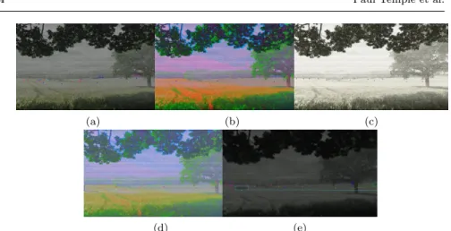
Figure 5 shows some examples of non-acceptable videos that can be gener-ated with MOTIV. On these images, there is noise preventing human beings
(a) (b) (c)
(d) (e)
Fig. 5: Examples of non-acceptable generated videos
to perceive the background and whether a vehicle is present and their identi-fications. In addition, for Figures 5a, 5c and 5e, contrast is poor while Figure 5b and 5d present unrealistic colors.
Non-acceptable videos represent a waste of time and resources: 30 minutes of CPU-intensive computations per video on average, without including the time to run benchmarks related to object tracking (several minutes depend-ing on the computer vision algorithm). We therefore need to constraint our variability model to avoid such cases.
Previous work. We previously used ML classification techniques to predict the acceptability of unseen video variants [86]. We summarise this process in Figure 6. We first sample valid configurations using a random strategy (see Temple et al. [86] for details) and generate the associated video sequences. Our testing oracle labels videos as acceptable (in green) or non-acceptable (in red). This oracle implements image quality assessment [35] defined by the authors via an analysis of frequency distribution given by Fourier transformations. An ML classifier (in the case of [86], a decision tree) can be trained on such labelled videos. “Paths” (traversals from the root to the leaves) leading to non-acceptable videos can easily be transformed into new constraints and injected in the variability model.
AdvML to the rescue. An ML classifier can make errors, preventing accept-able videos (false positives) or allowing non-acceptaccept-able videos (false negatives). Most of these errors can be attributed to the confidence of the classifier com-ing from both its design (i.e., the set of approximations used to build its decision model) and the training set (and more specifically the distribution of the classes). Areas of low confidence exist if configurations are very dissimilar to those already seen or at the frontier between two classes. In the reminder, we investigate the use of advML to quantify these errors and their impact on MOTIV SPL and ML classifier.
Variability model Sampling method Configuration files Generating the training set
…
Derivation (Lua generator)
Oracle (Video Quality Assessment) … Labeling Machine learning J48 tree signal_quality.luminance_dev signal_quality.luminance_dev signal_quality.luminance_dev capture.local_light_change_level 0 (110.0/1.0) 0 (2.0) 1 (27.0) 1 (4.0) 0 (3.0) > 21.3521 <= 21.3521 <= 1.01561> 1.01561 <=18.1437>18.1437 <=0.401449> 0.401449 Variability model + cst1 ^ cst2 ^ … Constraints Constraints extractor
Constraining the original variability model
Testing the training set
Separating model using machine learning
Fig. 6: Refining the variability model of the MOTIV video generator via an ML classifier. In this article and as a follow up of this engineering effort, our goal is to generate adversarial configurations capable of fooling the ML classifier. 4.2 JHipster
JHipster is an open-source generator for developing Web applications [47]. Started in 2013, the JHipster project is popular with more than 15,000 stars on GitHub and gathers a strong community of more than 500 contributors in December 2019. JHipster is used by many companies and governmental or research organisations worldwide, including Google, Ericsson, CERN or the Italian Research Council (CNR).
From a user-specified configuration, JHipster generates a complete tech-nological stack constituted of Java and Spring Boot code (on the server side) and Angular and Bootstrap (on the front-end side). The generator supports several technologies ranging from the database used (e.g., MySQL or Mon-goDB ), the authentication mechanism (e.g., HTTP Session or Oauth2 ), the support for social log-in (via existing social networks accounts), to the use of microservices. Technically, JHipster uses npm and Bower to manage depen-dencies and Yeoman8
(aka yo) tool to scaffold the application [73]. JHipster relies on conditional compilation with EJS9
as a variability realisation mecha-nism. The mechanism is similar to #ifdef with CPP preprocessor and is applied on different files written in different languages: Java, JavaScript, CSS, Docker files, Maven or Gradle files. The build process resolves variability scattered in numerous files and is quite costly (10 minutes on average per configuration).
Previous work. We previously used JHipster as a case study to benchmark sampling techniques and assess their bug-finding effectiveness [45, 69]. Lessons learned from our study are that building a configuration-aware testing infras-tructure for JHipster requires a substantial effort both in terms of human and computational resources. Specifically, we relied on 8 man-months for building the infrastructure and 4376 hours of CPU time as well as 5.2 terabytes of disk
8
http://yeoman.io/
9
space used to build and run all JHipster configurations. Another lesson is that our exhaustive exploration of JHipster variants is not practically viable.
AdvML to the rescue. Instead of deriving all variants, one can use ML and only a sample of configurations to eventually prevent non-acceptable variants and avoid costly build. Such effort can also be exploited as part of the continu-ous integration of JHipster. The process of Figure 6, illustrated for MOTIV, is conceptually similar for JHipster. We have a feature model documenting the possible configurations and materialized as configuration files. The variants (or products) are not videos this time, but variants of source code written in different languages. As an outcome, we can identify features of JHipster that cause non-acceptable variants (i.e., build failures) and re-inject this knowledge into the feature model. Build failures can occur in various circumstances such as: (1) implementation bugs in the artefacts, typically due to a dependency wrongly specified in a Maven file or due to unsafe interactions between fea-tures in the Java source code; (2) un-properly building environments in which some packages or tools are incidentally missing because some combinations of features were not assessed before. Once the learning process of Figure 6 is realized, the question arises as to the quality of the ML classifier and the whole JHipster SPL. Again, we can apply advML.
In this article, we use the version 4.8.2 whose reverse-engineered feature model is available online10
. The feature model allows one to build all JHipster configurations. Yet, in our sampling we made a few restrictions to focus on the most relevant ones. In particular, we selected all the testing frameworks (Gatling, Cucumber, Protractor ) in each sampled configuration and avoided configurations that required Oracle to focus on non-proprietary variants. This feature model allows 90,210 variants in total.
4.3 Cases Synthesis
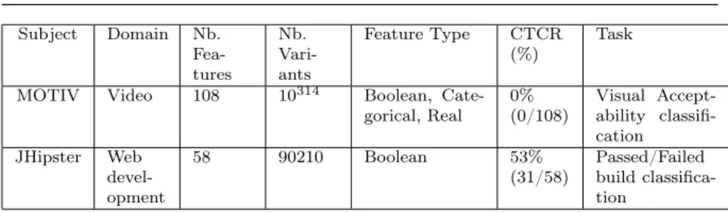
Table 1 summarises the main characteristics of the case studies analysed in this work. We notice that the domain greatly influences constraints stated in the variability model. While JHipster exhibits a high Cross-Tree Constraints Ratio (CTCR), proactively preventing the majority of build failures, MOTIV allows any combination of features, sometimes leading to unacceptable videos (soft constraints). From an adversarial machine learning perspective, MOTIV raises the challenge of navigating in a huge variability space with an imperfect oracle implementing visual perception. JHispter is requiring to handle constraints, specifically when running an evasion attack, since the risk of generating useless adversarial configurations is very high if we ignore them.
10
Subject Domain Nb. Fea-tures Nb. Vari-ants Feature Type CTCR (%) Task
MOTIV Video 108 10314 Boolean,
Cate-gorical, Real 0%(0/108) Visual Accept-ability classifi-cation
JHipster Web devel-opment
58 90210 Boolean 53%
(31/58) Passed/Failedbuild classifica-tion
Table 1: Case studies’ characteristics. We report for each case the domain, number of features and variants, the type of features, the Cross-tree constraints Ratio (CTCR) that is the number of features involved in cross-tree constraints to the total number of features and finally the goal of the classsification task.
5 Evaluation Overview
In this section, we introduce the research questions related to the use of ad-vML attacks for SPLs and present how we implemented them. The last part describes how we preprocessed data and the parameterization of the techniques used to run our experiments.
5.1 Research Questions
We address the following research questions:
RQ1: How effective is our adversarial generator to synthesize adversarial configurations? Effectiveness is measured through the capability of our evasion attack algorithm to generate misclassified configurations:
– RQ1.1: Can we generate adversarial configurations that are wrongly clas-sified?
– RQ1.2: Are all generated adversarial configurations valid w.r.t. constraints in the VM?
– RQ1.3: Is using the evasion algorithm more effective than generating ad-versarial configurations with random modifications?
– RQ1.4: Are attacks effective regardless of the targeted class?
RQ2: What is the impact of adding adversarial configurations to the train-ing set regardtrain-ing the performance of the classifier? The intuition is that addtrain-ing adversarial configurations to the training set could improve the performance of the classifier when evaluated on a test set.
We answer these questions for each case study separately in Sections 6 and 7. First, we state the evaluation protocol and then the results to these an-swers. We answer each question using both techniques presented in Sections 3.2 and 3.3. We also provide statistical evidence on the fact that our results are significantly different from results without using any advML technique. To do so, we performed Mann-Whitney tests as detailed in the evaluation protocol (see Section 5.4)
5.2 Implementation
We implemented the dedicated algorithm in Python 3 (scripts are available on the companion website).
MOTIV’s variability model embeds enumerations which are usually en-coded via integers. The main difference between the two is the logical order that is inherent to integers but not encoded into enumerations. As a result, some ML techniques have difficulties to deal with them. The solution is to “dummify” enumerations into a set of Boolean features, without forgetting to enforce inherent exclusion constraints of literals from the original enumer-ations. Conveniently, Python provides the get_dummies function from the pandas library which takes as input a set of configurations and feature indexes to dummify.
For each feature index, the function creates and returns a set of Boolean features representing the literals’ indexes encountered while running through the set of given configurations: if the get_dummies function detects values in the integer range [0, 9] for a feature associated to an enumeration, it will return a set of 10 Boolean features representing literals’ indexes in that range. The function takes care of preserving the semantics of enumerations. However, dummification is not without consequences for the ML classifier. First, it in-creases the number of dimensions: our 46 initial enumerations would map to 145 features that may expose the ML algorithm to the curse of dimensional-ity [13]; as the number of features increases in the feature space, configurations that look alike (i.e., with close feature values and the same label) tend to go away from each other, making the learning process more complex. This curse has also been recognized to have an impact on SPL activities [31]. Second, dummification implies that we will operate our attacks in a feature space es-sentially different from the one induced by the real SPL. Thus, we need to transpose the generated attacks in the dummified feature space back to the original SPL one, raising one main issue: there is no guarantee that an attack relevant in the dummified space is still efficient in the reduced original space (the separation may simply not be the same). For instance, dummification will break a categorical feature into multiple independent binary features. The attack will process each feature individually, it may result that two binary fea-tures to be activated at the same time as they are considered independently one from another. The original categorical feature implicitly encodes a de-pendency between all the available literals not reported by the dummification procedure and thus both feature space (i.e., before and after the transforma-tion) are not equivalent. Further efforts are required to ensure these implicit constraints.
Additionally, exclusion constraints stated in the FM and enumerations be-come non-correlated after dummification allowing gradient methods to operate on each feature independently. That is, when transposed back to the original configuration space, invalid configurations would need to be “fixed”, potentially putting these adversarial configurations away from the optimum computed by the gradient method. In the following, we will only perform transformations on
the initial feature space that can be reversed (e.g., normalize values between 0 and 1) to conduct our evasion attacks, the transition between the two feature spaces (i.e., initial and after preprocessing) is possible, thus, we do not make any further distinctions between the two terms since we use them without making any transformations.
As mentioned in Section 3.2, we conducted attacks on a SVM with a linear kernel which is a simple classifier (i.e., only linear separation can be created) but that performs already very well on the classification task for both case studies. Scripts as well as data used to compare predictions can be found on the companion webpage.
5.3 Presentation of the results
In sections 6 and 7, we present the results of our experiments for each RQs stated in Section 5.1. We try to keep the same structure for each addressed RQ, except for RQ 1.3 which is the comparison to random perturbations and does not use either of the implementations. First, we describe the preprocessing applied to the data and the parameterization of the two different implementa-tions of the evasion attack. Then we address each RQ by describing the intent and details about how we conducted our experiments and discussing the re-sults that come with an illustration. Finally, we provide some insights based on these results. We repeat the same schema for the second implementation. 5.4 Evaluation protocol
Data collection:Previous work on both case studies [86, 44,70] allowed one to gather a number of configurations (i.e., 90, 210 configurations from JHipster in its version 4.8.2. and 4, 500 randomly sampled and valid video configurations for MOTIV). Configurations were sampled, derived (executed or build), and assessed using a computing grid.
Training and Test sets:In the 4, 500 MOTIV configurations, about 10% are non-acceptable (see Section 4.1). Because of the vast majority of accept-able configurations, we are not accept-able to use common ML practices: usually, the training set is composed of a high percentage (e.g., around 66%) of avail-able data and is used to train the classifier, and, when few configurations are available, k-fold cross-validation is used to mitigate the risk of overfitting (in our case, 4, 500 configurations is an arguably low number to the size of the variant space). Regarding the number of configurations to put in the training set, 66% of 4, 500 configurations would reduce the size of the test set in turns containing very few non-acceptable configurations. In such a setting, because of the approximations explained in Section 3.3, the classifier can easily learn a function that will not separate anything while keeping good classification per-formances since non-acceptable configurations would be considered as “rare events” in numbers. Because of that, we decided to mitigate this risk by train-ing a classifier with even fewer configurations but keeptrain-ing the same ratio of
non-acceptable configurations (i.e., ≈ 10%) leading us to 500 configurations in the training set among which around 50 are non-acceptable. Results from [86] showed good results in terms of classification on both training and test sets which made us keep this setting.
Now, regarding cross-validation, it is used to validate/select a classifier when several are created (e.g., when fine-tuning hyper-parameters) but it requires separating the training set into smaller subsets. With 10% of non-acceptable configurations some subsets will not contain any of them which is counter-productive when assessing the ability of a trained classifier to successfully classify new configurations.
In this setting, the key point is that only about 10% of configurations are non-acceptable. This is a ratio that we cannot control as it depends on the targeted non-functional property. However, to reduce imbalance, several data augmentation techniques exist like SMOTE [27]. Usually, they create artificial configurations while maintaining the configurations’ distribution in the feature space. We decided to follow a similar process by computing the centroid between two configurations (of the same class) and use this point as a new configuration.
Thanks to the centroid method, we can bring a perfect balance between the two classes (i.e., 50% of acceptable configurations and non-acceptable con-figurations). Technically: we compute the number of configurations needed to have perfectly balanced sets (i.e., for both training and test sets); we select randomly two configurations from the less represented class and compute the centroid between them, check that it is a never-seen-before configuration and add it to the available configurations. The process is repeated until the re-quired number of configurations is reached. Once a centroid is added to the set of available configurations, it is available as a configuration to create the next centroid.
In the following, we present results with both original and balanced data sets to assess the impact of class representation on adversarial attacks.
On the other hand, JHipster presents about 20, 000 configurations in the dataset that cannot be built. This represents about nearly 25% of our dataset, which shows an over-representation of the building class. While other problems (described later on under the label Feature space structure) remain, this representation is still an issue and we had to force sets to be perfectly balanced. Thus, we chose to reduce the training set to 400 configurations. In this training set, both classes are represented equally (i.e., 200 configurations for each class). That is, we choose randomly 200 configurations from the ones that build and 200 other configurations from the ones that do not.
Preprocessing:We have applied some preprocessing to both datasets and configurations’ representations to remove unnecessary features gathered from our previous study. For instance, for JHipster, we removed logs that were kept for further studies to retrieve the root causes of bugs. They were stored as free text which prevented us to have an homogeneous representation of the configurations in terms of features. Furthermore, error messages from the logs are not necessary for this study. If a feature only reports one value, it is
discarded since it will only increase the number of dimensions in the feature space without adding any information to the classification problem.
Since we use SVMs to conduct evasion attacks, we need to make our fea-ture space homogeneous in its dimension. Integer values must be scaled-down between 0 and 1. The same applies to floating-point values. The reason be-hind this decision is to avoid unbounded values which in turn can result in bigger importance given to a feature because it is more flexible and can take a broader range of values. To cope with homogeneous feature spaces, we applied dummification (see Section 5.2) to categorical features. This way, every single literal of the feature becomes an independent Boolean feature.
After these preprocessing steps, MOTIV configurations are represented by about 120 features while JHipster’s configurations contain 47.
Feature space structure:Regarding JHipster, our preliminary study, to assess that at least one ML model was able to classify configurations between building or not building, showed that this classification problem is linearly separable. Even with as few as ≈ 18, 000 configurations (about 20% of available configurations) in the training set, the classifier as able to perform more than 99% of correct prediction in the test set. Below this number, our tentatives to learn a classifier with a random selection of configurations have often failed due to the absence of non-building configurations. With more than 99% accurate classifications, adversarial attacks were unable to produce any configurations that were misclassified by the classifier. Besides, unlike the MOTIV case study, after our feature transformation, JHipster presents numerous dependencies between the features (i.e., the choice of using a SQL database force to deselect any other kind of database) making the adversarial attacks unlikely to produce any valid configurations regarding the associated feature model. We add to enforce encoded constraints (choices, dependencies stated as constraints in the FM and upper and lower bounds values) in the FM directly into the attack procedure. That is, after the last displacement has been performed, we check that all the constraints are fulfilled and, if not, modify crafted configurations accordingly. This way, configurations produced by the adversarial procedure are valid by design. This is also known as the “fix operator” in configuration optimization [65].
Parameterization of the techniques: We configured the dedicated at-tack generator with the following settings: i) we set the number of atat-tacks points to generate 4, 000 configurations for RQ1 with MOTIV and 1, 000 when dealing with JHipster and, for RQ2, 25 configurations were used for both case studies; ii) considered step size (t) values are {10−6
; 10−4 ; 10−2 ; 1; 102 ; 104 ; 106
}; iii) the number of iterations is fixed to 20, 50 or 100. To mitigate ran-domness, we repeat ten times the experiments. All results discussed in this paper can also be found on our companion webpage11
.
When using secML, we have parameterized the attack function such that it can change several features at one time (distance norm is set to “l2” also known as Euclidean distance), the maximum perturbation value (called d_max
here-11
after) is set to {0.1; 0.5; 1.0; 5.0; 10.0} and the upper and lower bounds are set respectively to 1 and 0. Also, Gradient Descent uses a search grid to find the best step size as well as the best direction which can be configured by the reso-lution of the grid. In secML, this parameter is called η that we set to 0.01 since the order of magnitude of the number of features is 102
. To remain consistent with our dedicated implementation, we apply the same preprocessing on the configurations (see Section 5.2) and we generate 4000 configurations for RQ1 and 25 configurations when addressing RQ2.
Statistical Evidence: To further support the statistical validity of our conclusions we applied statistical tests for each research question. We focused on Mann-Whitney rank sum test [58], which is non-parametric (i.e., it does not assume a normal distribution for the compared samples) and therefore can han-dle the non-normality of our sometimes small sample sizes. This test computes a statistic U , further decomposed in U1 and U2that intuitively correspond to
the number of wins and losses respectively of all pairwise contests between the two compared samples. Therefore, 0 < Ui < n1× n2, i∈ {1, 2} where n1, n2
are the sizes of each sample and U1+ U2 = n1× n2. We report min(U1, U2)
referred to as “u-stat”. For this test, we formulate two different hypotheses: the null-hypothesis (usually called H0) that supposes the two samples follow the same distributions and the other hypothesis (H1) supposing that they do not. To reject the null-hypothesis, u-stats are compared to a critical value reported in a table12
: if a u-stat is smaller or equal to the one in the table for the given sample sizes and confidence levels (in our case α = 0.05), then we can reject H0, if it is greater then we cannot reject H0. Additionally, two values of u-stat are remarkable: u-stat = 0, meaning that the distributions are totally differ-ent, and u-stat = n
1×n2
2 meaning that the two distributions are equal. In our
setting, we use a two-tailed test and additionally report the computed p-value pfor significant (we consider our results significant if p ≤ 0.05). We computed our statistical results using the R statistical environment [72]. The R script to replicate the analysis can be found on our companion webpage.
6 MOTIV
6.1 RQ1: How effective is our adversarial generator to synthesize adversarial configurations?
To answer this question, we assess the number of wrongly classified ad-versarial configurations over 4000 generations and compare them to a random baseline: to the best of our knowledge, there is no other evasion attack that is based on a different algorithm than the one presented in [16] to compare to.
12 Such tables can be found easily on the Internet: http://ocw.umb.edu/psychology/
(a) Number of misclassified adversarial
con-figurations (20 displacements) (b) Number of misclassified adversarial con-figurations (100 displacements)
Fig. 7: Number of successful attacks on class acceptable; X-axis represents dif-ferent step size values t while Y-axis is the number of misclassified adversarial configurations by the classifier. For each t value, results with balanced and not balanced training set are shown (respectively in blue and orange).
6.1.1 RQ1.1: Can we generate adversarial configurations that are wrongly classified?
Dedicated implementation
For each run, after nb_disp displacements, the newly created adversarial con-figuration is added to the set of initial concon-figurations that can be selected to start an evasion attack. We thus allow previous adversarial configurations to continue their displacements towards the global optimum of the gradient.
Figure 7 shows box-plots resulting from ten runs for each attack setting. Both results, when the training set is not balanced (i.e., using the previous training set containing 500 configurations with about 10% of non-acceptable configurations) and when it is balanced (i.e., increasing the number of non-acceptable configurations using the data augmentation technique described above) are reported.
Both Figure 7a and Figure 7b indicate that we can always achieve 100% of misclassified configurations with our attacks. Regarding Figure 7a, in the case of a not balanced dataset, it is easy to attack the most represented class and the implementation can produce new configurations that are always misclas-sified (regardless of the value assigned to t). The fact that even the smallest value of t with 20 displacements can produce 4000 misclassified configurations suggests that the separation learned by the classifier should be very close to the configurations of class non-acceptable (where the attacks start). With a balanced dataset, more points can be selected as a starting point of the at-tack. Chances to select a starting point that is “far” from the separation are higher and more displacements are needed to cross the function learned by the classifier. Figure 7a shows that the displacement step size is not enough
to produce any misclassified configurations when it is set to a value lower or equal to 10−4
and the number of displacement is set to 20. When set to 0.01, some configurations start to be misclassified but it represents less than 50% of them. With a step size set to 1.0 or above, perturbations are large enough to produce misclassified ones.
Figure 7b shows the same tendency except that the transition from 0 mis-classified generations to 4000 appears earlier (i.e., when t is set to or close to 0.01). It is not surprising since, compared to the previous results, the number of displacements is higher (set to 100).
We do not present figures with the number of displacements set to 50 but the observations are similar to the ones we just described with Figure 7b. However, they can be found on the companion webpage.
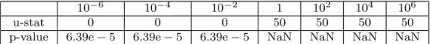
Table 2 shows U (second row) from the Mann-Whitney test and associated p-values (third row) when comparing results from both sets (balanced and unbalanced) for each displacement step size shown in Figure 7a. When the displacement step size is set to 1 or higher, both attack set-ups achieve a 100% success rate with no dispersion (illustrated by 50 and NaN values in the table) and therefore cannot be distinguished. With lower values of displacement step sizes, the p-values are significant (p << 0.05). Based on our results from Figure 7a, we can conclude that attacking when classes are not balanced is easier. Conclusions are similar when considering larger displacement step size (i.e., 50 and 100) available on the companion page.
10−6 10−4 10−2 1 102
104
106
u-stat 0 0 0 50 50 50 50
p-value 6.39e − 5 6.39e − 5 6.39e − 5 NaN NaN NaN NaN
Table 2: u-statistics and p-values associated with measures from Fig. 7a; n1=
n2= 10 for each column, u-statcritical= 23.
Insights: Increasing the number of displacements requires lower step sizes to reach the misclassification goal but it comes at the cost of more computations. However, increasing the number of displacements when the step size is already large ends up in incredibly large displacements which may not be realistic in some applications or when trying to limit changes applied to configurations.
SecML
Similarly to the previous implementation, after the final perturbation is ap-plied to a configuration, it is added to the set of available configurations that may be selected for the next run. The number of displacements is not bounded directly, thus the number of iterations can vary from one run to another.
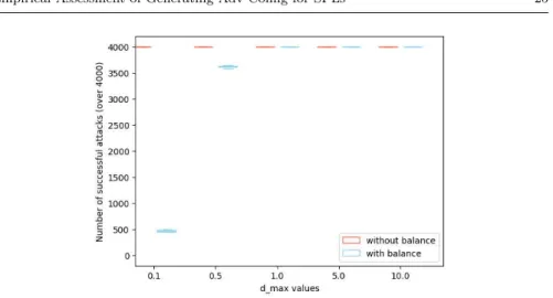
Figure 8 shows box-plots resulting of ten runs for each attack setting (i.e., with varying values set to d_max). We also show results for both balanced and non-balanced data sets.
Fig. 8: Number of successful attacks on class acceptable; X-axis represents different parameter values of d_max of the secML function while Y-axis is the number of misclassified adversarial configurations by the classifier.
When the data set is not balanced, similarly to the previous implemen-tation, all attempts to create a misclassified configuration succeed since the separation is in favor of the most-represented class.
When the data set is balanced, the behavior showed in Figure 8 is similar to the previous one. A transition from 500 misclassified generated configurations to almost 4000 can be seen between d_max set to 0.1 and 0.5. With higher d_max values, all 4000 generated configurations were misclassified.
Our statistics (available on Table 3) shows that our results are significant (p << 0.05). Again, with this implementation, we can conclude that attacking classes is easier when they are imbalanced.
0.1 0.5 1 5 10
u-stat 0 0 12.5 12.5 12.5
p-value 7.49e − 3 7.49e − 3 NaN NaN NaN
Table 3: u-statistics and p-values associated with measures from Fig. 8; n1=
n2= 5 for each column, u-statcritical= 2.
Insights: again tuning d_max increases chances to get misclassified con-figurations when perturbed with evasion attacks. Since d_max represents the maximum distance up to which a feature can be perturbed, setting it a lower value decreases the potential number of iterations to get to the final position. Therefore, to fine-tune this parameter, a good strategy would be to start with lower values.
6.1.2 RQ1.2: Are all generated adversarial configurations valid w.r.t. constraints in the VM?
As discussed in Section 5.2, we have performed some preprocessing on our data to make the learning with an SVM possible and reliable. This ends up with features that are either Boolean, either real but bounded between 0 and 1.
Because we check and force feature values to be inside these boundaries after the last position of a configuration is reached, by design, all the config-urations are valid w.r.t. this aspect. The only aspect left that may make the configurations non-valid is the mutual exclusion constraints inherited from breaking the categories with the dummification process.
Regardless of the implementation that is used or the values given to pa-rameters, all the generated configurations are valid. Results and scripts of this experiment can be found on the companion website.
Insights: We can scope parameters such that adversarial configurations are both successful and valid for either implementations. The way our configu-rations were preprocessed made it possible to enforce boundary constraints directly at the end of displacements. Other ways are possible but might re-quire other mechanisms to check that constraints are verified while allowing configurations to move further away.
6.1.3 RQ1.3: Is using the evasion algorithm more effective than generating adversarial configurations with random displacements?
Previous results of RQ1.1 and RQ1.2 show we can craft valid adversarial con-figurations that can be misclassified by the ML classifier but is our algorithm better than a random baseline?
The baseline algorithm is based on the dedicated implementation and con-sists in: i) for each feature, choose randomly whether to modify it; ii) choose randomly to follow the slope of the gradient or go against it (the role of ‘-’ of line 5 in Algorithm 1 that can be changed into a ‘+’); iii) choose randomly a de-gree of displacement (corresponding to the slope of the gradient (∇F (xm−1
)) of line 5 in Algorithm 1). Both the step size and the number of displacements are the same as in the previous experiments.
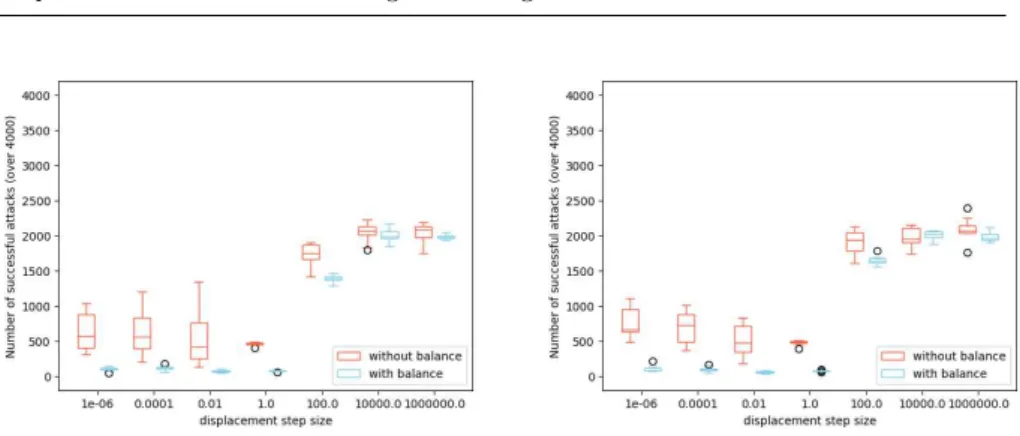
Figure 9 shows the ability of random attacks to successfully mislead the classifier. Random modifications are not able to produce more than 2500 con-figurations that are misclassified (regardless of the number of displacements, the step size, or whether the training set is balanced or not) which corresponds to about 60% of the generated configurations. It is a lower number than the two evasion implementations. The maximum number of misclassified configu-rations after random modifications starts from step size t = 10, 000 regardless of the studied number of displacements.
Regarding the validity of generated configurations, here again, the random version is worse than the other considered implementations. The problem lies
(a) Number of successful random attacks af-ter 20 displacements
(b) Number of successful random attacks af-ter 100 displacements
Fig. 9: Number of successful random attacks on class acceptable; X-axis rep-resents different step size values t while Y-axis is the number of misclassi-fied adversarial configurations by the classifier. In red and blue are respective results with a not balanced and a balanced training set in terms of classes representation.
in the fact that all features are processed independently from the others re-sulting in high chances to set to features which are mutually exclusive to 1; leading to non-valid configurations.
Table 4 shows the u-statistics and p-values when comparing results given from the RQ1.1 (see Figure 7a) and random perturbations (see Figure 9a) with balanced classes. For all reported values, the p-values are significant (p <<0.05) and U-stats are equal to 0. We conclude that advML techniques are more efficient in producing new configurations that will be wrongly classified than using random perturbations. Results are similar when comparing results from Figure 7b and Figure 9b.
10−6 10−4 10−2 1 102
104
106
u-stat 0 0 0 0 0 0 0
p-value 1.82e − 4 1.82e − 4 1.82e − 4 6.34e − 5 6.34e − 5 6.39e − 5 6.39e − 5
Table 4: u-statistics and p-values associated with measures from Fig. 9a com-pared with values given in RQ1.1 when classes are balanced; n1= n2= 10 for
each column, u-statcritical= 23.
Insights: Previous results show that the effectiveness of evasion attacks are superior to random modifications since i) evasion attacks can craft con-figurations that are always misclassified by the ML classifier while less than 2500 over 4000 generations will be misclassified using random modifications; ii) generated evasion attacks support a larger set of parameter values for which generated configurations are valid; iii) we were able to identify sweet spots for
![Fig. 1: Simplified MOTIV feature model [38, 4]](https://thumb-eu.123doks.com/thumbv2/123doknet/14488072.716953/6.892.112.611.116.347/fig-simplified-motiv-feature-model.webp)