HAL Id: tel-00451244
https://tel.archives-ouvertes.fr/tel-00451244
Submitted on 28 Jan 2010
HAL is a multi-disciplinary open access archive for the deposit and dissemination of sci-entific research documents, whether they are pub-lished or not. The documents may come from teaching and research institutions in France or abroad, or from public or private research centers.
L’archive ouverte pluridisciplinaire HAL, est destinée au dépôt et à la diffusion de documents scientifiques de niveau recherche, publiés ou non, émanant des établissements d’enseignement et de recherche français ou étrangers, des laboratoires publics ou privés.
GEOMETRY PROCESSING FOR COORDINATE
METROLOGY
Haibin Zhao
To cite this version:
Haibin Zhao. MULTISENSOR INTEGRATION AND DISCRETE GEOMETRY PROCESSING FOR COORDINATE METROLOGY. Mechanics [physics.medph]. École normale supérieure de Cachan -ENS Cachan, 2010. English. �tel-00451244�
N° ENSC-2010/???
THESE DE DOCTORAT
DE L’ECOLE NORMALE SUPERIEURE DE CACHAN
Présentée par Monsieur ZHAO Haibin
pour obtenir le grade de
DOCTEUR DE L’ECOLE NORMALE SUPERIEURE DE CACHAN
Domaine:
MECANIQUE - GENIE MECANIQUE - GENIE CIVIL
Sujet de la thèse:
MULTISENSOR INTEGRATION AND DISCRETE GEOMETRY
PROCESSING FOR COORDINATE METROLOGY
Thèse présentée et soutenue à Cachan le 18 Janvier devant le jury composé de:
M. J.-F. Fontaine Professeur - Université de Bourgogne Rapporteur M. J.-C. Léon Professeur - Grenoble INP Rapporteur M. P. Bourdet Professeur émérite -ENS Cachan Directeur de thèse M. N. Anwer Maître de conférences- Université Paris Nord Examinateur M. J. M. Linarès Professeur- Université de la Méditerranée Examinateur M. B. Hautbergue Directeur R&D – SPRING Technologies Invité
Laboratoire Universitaire de Recherche en Production Automatisée (ENS CACHAN / EA 1385)
The works proposed in this thesis are the fruits of the research activities in LURPA (Laboratoire Universitaire de Recherche en Production Automatisée) of ENS Cachan (Ecole Normale Supérieure de Cachan).
First of all, I want to give my great acknowledgements to my thesis director, Professor Pierre Bourdet. His profound knowledge and experiences guide my works under the correct direction. And his respectable personality also makes me feel pleasure during the three years when I stay in LURPA.
I address my unstinting appreciations to Nabil Anwer for his high quality supervising. Without him, I can’t reach the fruitful results of my research activities. He searched the opportunities for me to come in France to continue my Ph.D studies. During the whole three years, he gives me his great helps both in my academic research and in my living conditions. He also tried to find work opportunities for me after my graduation. For all of what he has already done for me, Thanks.
A great thankfulness is given to Prof. Jean-Jacque Lessage, who provides the opportunity and great conveniences for me to stay and study in the laboratory. The same thankfulness is also given to Prof. Luc Mathieu.
Thanks to Prof. Bernard Anselmetti and Prof. Claire Lartigue, who provide the opportunity and conveniences for me to stay and study in the team of Geo3D.
I want to thank Prof. Jean-Claude Paul and Prof. Wang Junying for their agreeable receptions during the ten months when I stayed in Tsinghua University, China. The same thankfulness is also given to Mr. Li and Mrs. Yang who work in CAD Teaching Center in Tsinghua University.
Thanks to the office of SRI (Service des Relations Internationales) of the ENS Cachan who provides the financial support to my first year staying in France. Thanks to the Sino-French Laboratory PLMIC (PLM Innovation Center) who finances me the second year of my research works in China. And thanks to LURPA, who supports me the finances needed for my third year in France.
Thanks to all the members in LURPA. They give me their sincere assistances which make feel comfortable during the periods I spend in LURPA. The periods I stayed in France are amazing and very important for me. Great thanks to Nicolas Audfray who assists me to do the experiments. Great thanks also to Laurant Tappie, Charyar Mehdi-Souzani, Renaud Costadoat, et al. who provide the testing models and contributions to the thesis. My great thankfulness is also given to Labib Daoud, who provides his kind helps to solve my academic and living difficulties during my staying in France.
Thanks to Dr Yang Jianxin who is now working in LURPA. As one of my senior fellow apprentice in Tsinghua University, He gives me his sincere helps both in research and in living. Thanks. I also want to thank my Chinese friends living in ENS Cachan and living in Paris, who provide their helps for me. It is pleasure to share my time with them.
Finally, I prefer to give my heartfelt appreciations to ZHANG Min, and also to my parents, my sisters and my other kindred. Thanks for their selfless supports and encouragements in my life.
Introduction...1
Chapter 1: Multisensor Integration in Coordinate Metrology ...7
1.1. Introduction...8
1.2. Sensing techniques for coordinate metrology ...9
1.2.1. Contact probing...9
1.2.2. Laser range triangulation...13
1.2.3. Chromatic confocal imaging ...17
1.3. Multisensor integration in coordinate metrology ...22
1.3.1. Multisensor configuration ...22
1.3.2. Multisensor data fusion ...23
1.3.3. Related works in multisensor integration...24
1.4. Development of an integrated multisensor system for coordinate metrology...32
1.5. Conclusion ...33
Chapter 2: Function and Data Modeling for Multisensor Integration ...35
2.1. Introduction...36
2.2. Functional analysis of the system...36
2.2.1. Function modeling using IDEF0 ...36
2.2.2. Function models ...38
2.2.3. Conclusion...51
2.3. Ontology-based data modeling...52
2.3.1. Introduction to ontology modeling...52
2.3.2. Data modeling ...55
2.3.3. Ontology development ...61
2.3.4. Conclusion...63
2.4. Conclusion ...64
Chapter 3: Discrete Differential Geometry ...65
3.1. Introduction...66
3.2. Polyhedral surface approximation...67
3.2.1. Approximation method and mesh data generation...67
3.2.2. File formats for mesh data representation and exchange ...70
3.3. Differential geometry properties Estimation ...72
3.3.1. Differential geometry of smooth surface...72
3.3.2. Normal vector estimation ...76
3.3.3. Discrete curvature estimation methods ...79
3.3.4. Our estimation method ...85
3.3.5. Shape index and curvedness...86
3.5. Conclusion ...94
Chapter 4:Registration of Discrete Shapes...95
4.1. Introduction...96
4.2. Literature review ...96
4.3. Method overview ...98
4.4. Coarse registration ...100
4.4.1. Principal pose estimation ...100
4.4.2. Transformation calculation...102
4.4.3. Overlapping alignment...104
4.5. Fine registration ...108
4.5.1. Flow chart of the CFR method...108
4.5.2. Geometric distance definition ...110
4.5.3. Corresponding point pairs searching... 111
4.5.4. Corresponding point pairs registration ...112
4.5.5. Convergence condition...115 4.6. Testing results...116 4.6.1. Full-full overlapping ...116 4.6.2. Full-partial overlapping...117 4.6.3. Partial-partial overlapping...118 4.6.4. Performance analysis...120 4.7. Conclusion ...127
Chapter 5:Discrete shape recognition and segmentation ...129
5.1. Introduction...130
5.2. Literature review ...130
5.3. Method overview ...134
5.4. Local surface type recognition ...137
5.4.1. Surface types based on Gaussian and mean curvatures...137
5.4.2. Surface type definition based on shape index ...137
5.5. Vertex clustering...141
5.5.1. Sharp edges and high curvature regions detection ...141
5.5.2. Vertex clustering and cluster refining...143
5.6. Connected region generation...148
5.6.1. Connected region labeling...149
5.6.2. Region visualization...151
5.6.3. Region merging and refining...153
5.7. Experiments and Results ...156
5.7.1. Testing cases...157
5.7.2. Noise effect ...161
5.7.3. Time performance ...163
Chapter 6: A Case Study ...171
6.1 Introduction...172
6.2. Multidata acquisition...172
6.2.1. Multisensor system configuration ...172
6.2.2. Data acquisition...179
6.3. DSP-COMS platform overview ...180
6.3.1. Main interface ...181
6.3.2. Menu specification ...182
6.4. Discrete geometry processing ...184
6.4.1. Registration ...184
6.3.2. Segmentation...188
6.5. Conclusion ...191
Conclusion ...193
Figure 1-1: Classification of the sensing techniques for coordinate metrology...9
Figure 1-2: Limitations of the touch probing system with considering the tip size ...10
Figure 1-3: Coordinate systems in contact probing systems...11
Figure 1-4: Triangulation principles of laser scanning...13
Figure 1-5: Modeling of the laser scanning system on CMM platform...15
Figure 1-6: Working principle of chromatic confocal imaging system...19
Figure 1-7: Modeling of the STIL sensor mounted on CMM platform ...20
Figure 1-8: Calibration of the STIL sensor ...22
Figure 1-9: Three sensors configurations in multisensor systems...23
Figure 1-10: Interface standards in dimensional metrology systems [Hor05] ...30
Figure 1-11: The constructed system layout of the multisensor system...32
Figure 2-1: Graphic format of IDEF0 ...37
Figure 2-2: Hierarchical decomposition of IDEF0 diagrams...38
Figure 2-3: Top-layer IDEF0 diagram of the system – A-0 diagram ...39
Figure 2-4: A0 diagram – the first layer of the hierarchical structure...41
Figure 2-5: A2 diagram for measurement strategies planning ...44
Figure 2-6: Two trajectory generation methods ...47
Figure 2-7: A4 diagram for discrete geometry processing ...48
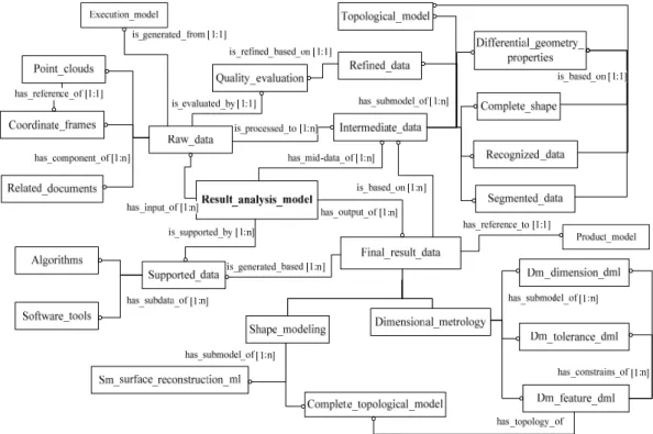
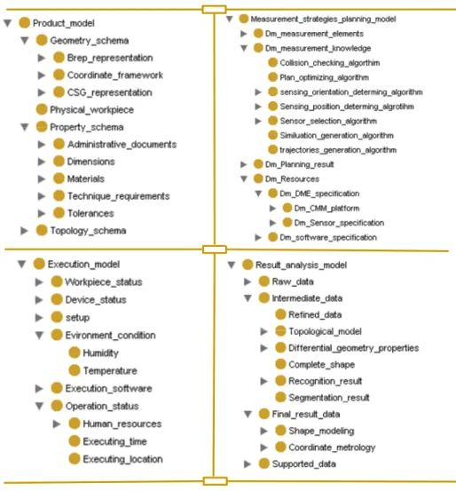
Figure 2-8: Product model ...57
Figure 2-9: Measurement strategies planning model (MSP model)...58
Figure 2-10: Execution model...59
Figure 2-11: Result analysis model...61
Figure 2-12: Top hierarchical structure of ontologies built on Protégé-OWL ...62
Figure 2-13: Ontology editing...63
Figure 3-1: Examples of the triangle mesh generation ...68
Figure 3-2: Schematic diagram of the half-edge data structure ...69
Figure 3-3: STL file format and a typical STL model...70
Figure 3-4: OFF file format and an example of OFF model...72
Figure 3-5: Normal and principal curvature directions of a smooth surface at point p ...75
Figure 3-6: The notations mentioned in normal estimation ...78
Figure 3-7: Two main types of local regions...81
Figure 3-8: The notations in the method of Cohen-Steiner and Morvan...85
Figure 3-9: The notations in our proposed method ...86
Figure 3-10: Three examples of the Normal estimation...88
Figure 3-11: The maximum and minimum principal curvature fields ...93
Figure 3-12: Time performance of our curvature estimation method ...94
Figure 4-1: Procedures of the proposed registration method ...99
Figure 4-2: Principal coordinate systems of two discrete shapes...102
Figure 4-3: Notations for coordinate system transformation calculation...103
Figure 4-4: Full overlapping alignment based on principal poses ...105
Figure 4-8: General registration flow of the CFR method ...109
Figure 4-9: Full-full overlapping registration of the armadillo data ...117
Figure 4-10: Full-partial overlapping registration of the Chinese dragon data (Dragon 1) ...118
Figure 4-11: Partial-partial overlapping registration of the Chinese dragon data (Dragon 2)...119
Figure 4-12: Partial-partial overlapping registration of the Stanford bunny data ...120
Figure 4-13: Partial-partial overlapping registration of the future Buddha data ...120
Figure 4-14: The two data used to test the influence of λ on registration performance...124
Figure 4-15: Registration of unitary shapes ...125
Figure 4-16: Registration of the data without sufficient correspondences...125
Figure 5-1: Procedures overview of shape recognition and segmentation...135
Figure 5-2: The locations of the surface types on shape index scales and their color scales ...139
Figure 5-3: Representative shapes of the 10 defined surface types based on shape index...139
Figure 5-4: Discrete shapes and their local surface types’ visualization...140
Figure 5-5: Example of mislabeling of sharp edge and high curvature region ...141
Figure 5-6: Curvedness maps of two discrete shapes ...142
Figure 5-7: Detection of the points in sharp edges and high curvature regions ...143
Figure 5-8: General flow of the proposed clustering algorithm...145
Figure 5-9: The defined surface types on the κ κ1− 2 plane...146
Figure 5-10: Examples of vertex clustering and cluster refining ...148
Figure 5-11: Studied cases for the connected region labeling...150
Figure 5-12: Four conditions a triangle possibly encountered for visualization ...152
Figure 5-13: Region label adjusting for visualization...153
Figure 5-14: Connected region merging and refining ...156
Figure 5-15: Boundary types in continuous and discrete shapes ...158
Figure 5-16: Segmentation of regions surrounded by sharp edges ...159
Figure 5-17: Segmentation of regions surrounded by tangent edges ...160
Figure 5-18: Segmentation of regions surrounded by curvature edges...161
Figure 5-19: Segmentation of complex shapes ...162
Figure 5-20: Segmentation of a discrete shape with noise...163
Figure 5-21: The tested discrete shapes in table 5-3 ...164
Figure 5-22: Shape used for testing the time performance ...165
Figure 5-23: Time performance of the testing case with different tessellations...166
Figure 5-24: Characteristic points identification from complex shapes...167
Figure 5-25: Limitations to the measured noisy point data...167
Figure 5-26: Segmentation with different sizes of vertices...168
Figure 6-1: The multisensor measurement system in LURPA ...173
Figure 6-2: The component to install the STIL pen on CMM arm ...177
Figure 6-3: Two configurations of the sensor physical integration...177
Figure 6-4: Automotive water pump cover ...179
Figure 6-5: Measurement system configuration and examples of the acquired data ...180
Figure 6-9: Coarse registration results in case 1 ...185
Figure 6-10: Fine registration results in case 1 ...185
Figure 6-11: The scene data and the model data in case 2 ...186
Figure 6-12: Coarse registration results in case 2 ...186
Figure 6-13: Fine registration results in case 2 ...186
Figure 6-14: The scene data and the model data in case 3 ...187
Figure 6-15: Coarse registration results in case 3 ...187
Figure 6-16: Fine registration results in case 2 ...188
Figure 6-17: Final discrete shape of the workpiece ...188
Figure 6-18: The maximum principal curvature map of the workpiece...189
Figure 6-19: The minimum principal curvature map of the workpiece ...189
Figure 6-20: The shape index map of the workpiece ...190
Figure 6-21: The curvedness map of the workpiece ...190
Figure 6-22: Recognition results of the high curvature points...191
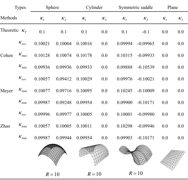
Table 3-1: Surface types specified by shape index intervals and their type labels...87
Table 3-2: Estimation of curvature values by the three methods on different surface types...90
Table 3-3: Estimation errors of the three methods on different surface types...91
Table 3-4: Sorting the methods based on the relative average error ...91
Table 3-5: Sorting the methods based on the relative maximum error...91
Table 3-6: Sorting the methods based on the relative minimum error ...92
Table 3-7: Time performances for the mentioned models...93
Table 4-1: Computational costs in coarse registration ...121
Table 4-2: Time performances of the tested cases in coarse registration ...122
Table 4-3: Time complexities of the two compared methods ...123
Table 4-4: Performances of the two compared algorithms...123
Table 4-5: The performances of the proposed method with different values of λ...126
Table 5-1: Surface types specified by signs of Gaussian and mean curvatures ...137
Table 5-2: The denotations used in connected region labeling ...149
Table 5-3: Computing times for the tested cases...164
Table 5-4: Computing times for the same shape with different tessellations...166
Table 6-1: Specifications of the Kreon Zephyr KZ25 laser scanner ...174
Table 6-2: Specifications of the Renishaw TP2 touch trigger probe...174
Table 6-3: Specifications of the STIL CL2 optical pen with CHR150 controller ...175
Acquiring 3D point data from physical objects is increasingly being adopted in a variety of product development processes, such as quality control and inspection [WRS00], reverse engineering [VMC97], etc. In coordinate metrology, many sensing technologies are available for data acquisition, such as tactile probing, laser scanning, confocal imaging, etc. In general, different sensors capture the information with different details. The complex design specifications are increasingly required to embed them in the mechanical parts such as shapes and surfaces description, dimensions, macro and micro geometrical tolerances, material characteristics for either functional or aesthetical reasons. It becomes difficult to satisfy all the measurement requirements with only a single sensor in coordinate metrology. An individual sensor can get neither holistic information of a workpiece accurately, nor spatial and temporal coverage with small measurement uncertainties in such measurement. Multiple sensors are hence employed to achieve both holistic geometrical measurement information and improved reliability or reduced uncertainty of measurement data [WJS09].
A multisensor integration system provides efficient solutions and better performances than the single sensor based system. Significant efforts are being devoted to the development of multisensor integration system in coordinate metrology. Different information sources (sensors) should be integrated in one common system. This makes complex system development to achieve the multisensor integration. Another fundamental question is how to merge the data provided by multiple sensors together and process them to extract meaningful geometric information.
In this dissertation, we investigate the multisensor integration and discrete geometry processing for coordinate metrology from two main parts: function and data modeling, and discrete geometry processing.
In order to achieve the multisensor integration, a comprehensive function and data modeling of the system are necessary to obtain clear and unambiguous understanding of the whole system. The system can be developed with the guidelines of the consistent function models and unambiguous data representation.
In multisensor integration system, the multiple sensors should be configured properly to fulfill the measurement. The specifications of the integrated sensors are usually different. The products measured by multisensor integration system usually
comprise complex specifications. The discrete geometry processing methods are also required for the achievement of multisensor integration.
A multisensor integration system contains various information and data. They should be described and managed unambiguously. The system should be also integrated with a PLM (Product Lifecycle Management) context, which also requires a unified and consistent data representation. Ontology development provides an effective way to represent and manage the data and the knowledge of multisensor integration system in coordinate metrology.
Multisensor integration requires suitable methods and algorithms of discrete geometry processing to process the multiple data acquired from different sensors. The methods in the three important phases of discrete geometry processing are investigated in this dissertation: normal and discrete curvature estimation; registration; shape recognition and segmentation.
Reliable estimation of normal and discrete curvatures is often required in many applications when the surface is defined by a set of discrete points rather than by mathematical formulae [MW00]. It is an essential task for discrete shape modeling and processing. Reliable estimation of discrete curvatures is also the basis of discrete shape registration and segmentation.
Registration is one of the most important and decisive steps of multisensor integration. The point data acquired by multiple views/sensors are usually represented in their own coordinate systems. During the registration process, the measurement data captured in the respective sensor’s coordinate system are aligned and transformed to one common coordinate system. The complete shape of the measured workpiece is generated after the registration process.
Recovering and extracting the useful information from discrete shapes play critical roles in discrete shape modeling domain. Generally, the shape recognition and understanding processes are based on the decomposition of the data into smaller parts [She08]. The shape recognition and segmentation are the most critical parts of discrete shape processing [VMC97]. Many applications including classification [JM07], object recognition [DGG04, SP08], reverse engineering [AMF00, BV04, DVV07, WKW02 YL99], and dimensional metrology [LX08, SHM01] need to solve the shape recognition and segmentation problem.
Contributions
The goal of this thesis is to investigate the multisensor integration and geometry processing in the context of coordinate metrology. The main contributions of the thesis are:
y A set of function models to analyze the functional requirements of multisensor integration system in coordinate metrology
y A Structured data modeling method based on ontologies for data representation and sharing.
y A set of methods to estimate the normal and the discrete curvatures of polygon mesh
y A set of methods for registration of multidata represented by respective sensors’ coordinate systems.
y A set of methods for discrete shape recognition and segmentation. y A developed software framework for discrete geometry processing.
Outline
The thesis is organized as follows:
Chapter 1 introduces three sensing techniques commonly used in coordinate metrology. The multisensor configurations and multidata fusion procedures, as well as the related works in multisensor integration for coordinate metrology are discussed. The layout of the developed multisensor measurement system is also presented.
Chapter 2 presents the detailed function model and data model of the developed multisensor integration system in coordinate metrology. The hierarchical decomposition of the function model is specified in details. An ontology based data model is developed to manage the various data in the developed system according to the different measurement stages defined by function model.
Chapter 3 proposes the methods to estimate normal vectors and curvatures of discrete shapes. The normal vector at each vertex is estimated from the normal vectors of the triangle facets in its neighbor region. A tensor based method is used to estimate the principal curvatures of discrete shapes. Two surface descriptors, shape index and
curvedness, are also introduced.
Chapter 4 presents a method to register the discrete shapes with unknown correspondences. The method uses the combination of the curvatures’ information and Euclidean distance to help the corresponding point searching. The method can provide accurate registration results with fast convergence. A comparative analysis of the proposed method and the initial ICP (Iterative Closest Point) algorithm is discussed in this chapter.
Chapter 5 presents new methods for discrete shape recognition and segmentation. Finally, several contributions are made in local surface type recognition based on shape index; vertex clustering and connected region partition. The methods provide satisfying results for segmentation of discrete shapes. The time performances of the proposed methods are also analyzed.
Chapter 6 presents a detailed case study of an industrial workpiece -automotive water pump cover. The multisensor integration platform and the measurement strategies of the workpiece are described. The developed software DSP-COMS, which serves as the test platform for the algorithms developed in this thesis. The detailed processing results of the studied workpiece are presented.
In conclusion, we summarize the thesis and propose some promising directions for the future research.
Chapter 1
Multisensor Integration in
Coordinate Metrology
1.1. Introduction
Acquiring 3D point data from physical objects is increasingly being adopted in a variety of product development processes, such as quality control and inspection [WRS00], reverse engineering [VMC97], etc. Complex shaped parts and tighter tolerances are increasingly required in modern engineering applications, either for functional or aesthetical reasons. The geometric specifications embedded in these parts such as shapes and surfaces, dimensions, macro and micro geometrical tolerances, material characteristics make it difficult to satisfy all the measurement requirements with only a single sensor in coordinate metrology. An individual sensor can get neither holistic information of a workpiece accurately, nor spatial and temporal coverage with small measurement uncertainties. Multiple sensors are hence employed to achieve both holistic geometrical measurement information and improved reliability or reduced uncertainty of measurement data [WJS09].
A multisensor integration system in coordinate metrology is a measurement system which combines several different sensors so that the measurement result can benefit from all available sensor information and data. With multisensor integration system, particular features of a workpiece can be measured with the most suitable sensor, and the measurement with small uncertainty can be used to correct data from other sensors which exhibit relevant systematic errors but have a wider field of view or application range.
This chapter introduces different sensing techniques commonly used in coordinate metrology and surveys the related work in multisensor integration. The integrated multisensor measurement system developed in our laboratory is also presented.
This chapter is organized as follows:
Section 1.2 introduces the different sensing techniques for surface digitizing in coordinate metrology. Section 1.3 discusses the multisensor configuration and data fusion process in multisensor methods. A comprehensive survey of related work in multisensor integration is presented in section 1.3. Section 1.4 describes the layout of the developed multisensor system for coordinate metrology.
1.2. Sensing techniques for coordinate metrology
Different sensor technologies are available for surface digitizing in coordinate metrology. According to their working principles, the sensing techniques for data acquisition in coordinate metrology can be classified into two categories: contact and non-contact [VMC99, CN04]. Figure 1-1 gives an overview of this classification..Figure 1-1: Classification of the sensing techniques for coordinate metrology
In the following sections, three data acquisition techniques that are widely used and cover different measurement scales are presented. Their working principles coordinate frames and calibrations are discussed below.
1.2.1. Contact probing
(1). Probing
principle
Contact probing systems are usually applied in cases where surface measurements allow or require lower point data density, such as the inspection of prismatic objects, known surfaces. The measuring ranges span from about a micrometer to several millimeters in one, two or three dimensions [WJS09]. The contact probing sensors are usually slow (1~2 point per second). Other limitations of the probing system are that the regions will be inaccessible if the sizes of these regions are smaller than the
diameter of the tip ball or that the peaks might lead to smoothed approximation of the surface (see the blue regions in figure 1-2 (1)). Moreover, the different sizes of the stylus tips also influence the measurement results (see figure 1-2(2)) [WJS09].
(1) Inaccessible regions (2) Influence of the different tip sizes Figure 1-2: Limitations of the touch probing system with considering the tip size
However, the accuracy of contact probing sensor is higher. The contact probing sensor is more adaptive to the environment and simple.
The working principle of contact probe is based on a mechanical interaction. There are two models: touch trigger and scanning.
The touch trigger mechanism will generate a trigger signal when the stylus is deflected away from its fixed seated position. The trigger signal generated by the probe in real time will be processed to record the position of the contact point in the three axes. Hence, the touch trigger probing contains two basic steps. The first one is approaching the measuring point on the surface to generate the trigger signal. And then followed by a withdrawing procedure in which the probe is back off the surface, the stylus returns to its initial position and is ready for next point probing. According to different sensor structures, this mechanism can be decomposed into three types: Kinematic resistive probing (i.e. Renishaw TP20 stylus), Stain-gauge probing (i.e. Renishaw TP7M stylus), and Piezo shock sensing (i.e. Renishaw TP800 stylus) [Ren].
On contrast, in scanning mechanism, the probe tip is always in contact with the surface during the measurement process. The touching element is guided on a curve along the surface while a set of coordinates are sampled in a time sequence [WSJ09]. The scanning mechanism works based on passive sensing (i.e. Renishaw SP600) or active sensing (i.e. Zeiss VAST system) technologies [Ren, WEP04].
In general, the scanning sensors are more complex in structure, data analysis and monitor control than the touch trigger sensors. The points acquired by scanning sensors (up to 500 points per second) are much more than the trigger sensors, but with
more uncertainty [WJS09]. Accordingly, the scanning sensors are suitable to perform the measurement of size, position and profile of precise geometric features, while the touch trigger sensors can be employed for prismatic parts without significant variations.
(2).
Modeling of the contact probing system
A contact probing system is a 3D data acquisition system in general, which means that the initial acquired data are 3D with (x, y, z) coordinates along the axes. The geometrical information can be derived from these 3D data. Most often, the functional characteristics of the contact probing systems can be derived from a Cartesian cylindrical or a spherical coordinate system. The probing process requires the definition of the coordinate systems for data acquisition. There are three coordinate systems in a 3D contact probing system [LG04, Ren] as shown in figure 1-3.
PCS MCS m O w O p O A r r A r b w r c r p r WCS PCS MCS m O w O p O A r r A r b w r c r p r WCS
Figure 1-3: Coordinate systems in contact probing systems
When a workpiece coordinate system (WCS) is defined on a workpiece, all the measured points can be output as rA after transformation from the machine
coordinate system (MCS) into WCS. From the relationships described in figure 1-3, the final result of rA can be derived as follows.
The coordinates of the point A in MCS is represented as:
A r p b
r = + + r r (1-1)
w
r can be represented as:
w c A
A r p c
r = + + − r r b r (1-3)
Where, rA is the position vector of the probed point A in workpiece
coordinate system. rr is the position vector of the origin of the probe coordinate
system in machine coordinate system. rc denotes the position vector of the origin of
the workpiece coordinates system in machine coordinate system. rw stands for the
point vector of the probed point in machine coordinate system. rp is the position
vector of the center of the probe tip in the probe coordinate system. and b denotes the radius vector which starts from the center of the tip and ends at the contact point.
(3).
Calibration of the probing system
Before inspection, the position of the center point of the probe tip related to the reference point (rpin figure 1-3) and also the radius of the tip ( b in figure 1-3)
should be known first for a correct measurement [EW96]. This is the main purpose of a calibration process. Many factors influence these parameters, such as probing force, pre-traveling of the probe, elastic attribute of the probing system, temperature and other parameters [Ren].
The calibration can be done by experiments with a calibrated artifact to determine the compensations for each influencing factor in the probing system. The most common used calibrated artifact is a sphere [WEP04]. Because the great varieties of the different probing systems, the calibration process is also done in different strategies. However, for each stylus needed to be calibrated in the system, the general calibration strategy is composed of the following steps:
(a) Selecting the calibrated artifact (with the same condition).
(b) Choosing the location and orientation of the artifact.
(c) Determining the number, location and sequence of the probing points on the artifact.
With the probed points, the experimental position and the tip ball size can be derived by surface fitting and the parameters can be compensated for the final data acquisition from the workpiece.
1.2.2. Laser range triangulation
(1).
Principles of laser scanning
The laser scanner can acquire a high density of point data from the surface with high speed. Its non-contact nature makes it suitable to measure the surfaces with flexible or soft materials [SNK02]. Even the laser scanner has its own demerits, such as limited viewpoint, occlusion, and sensitiveness to the surface optical conditions (specular for example), noise and redundancy in the acquired data, the laser scanners are frequently employed in coordinate metrology [NYH97].
The laser scanner works based on optical triangulation. With the triangulation principle, a point on the measured object can be determined by the trigonometric relations between the projector, the camera, and the object itself [WRS00]. The basic spot triangulation principle in 1D is shown in figure 1-4 (1). The depth distance d can be calculated as the formula (1-4):
sin sin sin( ) d b α β α β ⋅ = ⋅ + (1-4)
Where, b is the basic distance between the projector and the camera, which is a known physical parameter with a given laser scanner. α and β are the angles of the projector and the camera respectively.
Projector Camera Workpiece b d β α (1) Triangulation in 1D (2) Triangulation in 2D Figure 1-4: Triangulation principles of laser scanning
The spot scanner only captures the depth information of a single point each time. it needs to move in two directions for whole surface measurement. The point scanning in 1D is limited in accuracy and efficiency. Hence, the laser range scanner in 2D is
to intersect the object and so a profile stripe can be acquired in each time, as shown in figure 1-4 (2). The calculation of each point on the scan line is similar as the spot triangulation. However, a whole line or profile is measured in each time rather than only a single point. The accuracy and efficiency are both improved greatly.
The accuracy of a laser scanner is usually related to many factors, such as the relative position of the scanner and the object, the view angle, the condition of the measured surfaces, etc.. Some authors have already done some research works on that domain [GCB07, ML08].
(2).
Modeling of the laser scanning system on CMM platform
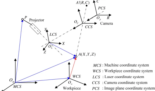
The laser range scanner is a 2D sensor. In each scanning, the scanner acquires a line image (represented by two dimensional parameters, such as (R, C)). Each point on the scanner line may correspond to a series of points on the object. An extrinsic calibration is therefore necessary to transform the 2D image data into 3D spatial data to represent the object naturally.The laser scanner is usually mounted on a CMM platform or on a robotic arm when doing the data acquisition. In our research, we consider the Laser scanning system integrated on CMM platform. There are five basic coordinate systems in the scanning system [LBM04] as shown in the figure 1-5.
(a) Machine coordinate system (MCS) is associated with the CMM.
(b) Workpiece coordinate system (WCS) is the reference coordinate system of the workpiece when the workpiece is in the design stage.
(c) Laser coordinate system (LCS) is constructed on the laser light plane virtually during the scanning. The origin of LCS is the intersection point between the optical axis of the camera lens and the laser light plane. The z-direction is along the normal of the laser light plane. And the x-, y-directions are the projections of the two perpendicular directions of the imaging plane of the camera, see the figure 1-5.
(d) Camera coordinate system (CCS) is the coordinate system associate with the camera lens. The origin of CCS is the center of the lens and z-direction is along the optical axis of the lens. The x-, y-directions are the projections of image plane matrix.
(e) Image plane coordinate system (PCS) is the coordinate system of the camera on the image plane. The z-direction is along the optical axis. and the x-, y- directions
are represented as (R, C). R and C denote the lines and the columns of the CCD matrix respectively. Hence, the coordinates of a point on image plane can be referred as ( ,R Ci i). MCS WCS LCS CCS PCS m O w O L O C O p O MCS WCS LCS CCS PCS ( , , ) A X Y Z '( , ) A R C P R C Z X Y
Figure 1-5: Modeling of the laser scanning system on CMM platform
Considering a point A on the surface, the three coordinates of A can be represented with WCS. The point A can also be represented with LCS. Therefore, we can get:
w w m m L L
O A=O O +O P+PO +O A (1-5)
Where, the point P in formula (1-5) and in figure 1-5 is the reference point of the laser scanner fixed on the CMM arm. The coordinates of P are represented in MCS as O Pm . O Ow m and POL generate the translation vectors. O AL represents
the position vector of A in the coordinate system LCS.
Considering the coordinates transformation between the two systems, WCS and LCS, we can obtain the following equations:
w lw L lw
O A=R O A T+ (1-6)
Where, Rlw is the 3 3× rotation matrix from LCS to WCS while Tlw is the
3 1× translation matrix.
systems LCS, CCS and PCS should be formulized. According to [LBM04], the final relationship between LCS and PCS can be expressed as:
' ( )
p L
O A =G O A (1-7)
Where, A denotes the imaging point corresponding to A . And so ' O Ap '
represents the position vector of A in PCS, which can be specified as (' R CA, A).
Considering the coordinates on the three axes of A in LCS, The equation (1-2-7) can be represented as:
1 1 ( , ) ( , ) 0 L A X A A L A Y A A L A X G R C Y G R C Z − − ⎧ = ⎪ = ⎨ ⎪ = ⎩ (1-8) Where, 1()
G− is the inverse function of G().
Finally, the coordinates of the point A represented in WCS which can be viewed the measured point data can be obtained from the following formula:
1 1 ( , ) ( , ) 0 1 0 1 1 W A X A A W lw lw A Y A A W A X G R C R T Y G R C Z − − ⎡ ⎤ ⎡ ⎤ ⎢ ⎥ ⎡ ⎤⎢ ⎥ ⎢ ⎥ = ⎢ ⎥⎢ ⎥ ⎢ ⎥ ⎣ ⎦⎢ ⎥ ⎢ ⎥ ⎢ ⎥ ⎣ ⎦ ⎣ ⎦ (1-9)
The method to calculate the parameters mentioned in formula (1-9) can be found in a calibration process.
(3).
Calibration of the laser range scanning system
The calibration considered here is the extrinsic calibration which is mainly used to determine the transformation relationships between the 2D image data in CCD space and the 3D spatial coordinates.
Considering the laser range sensor implemented in our experiments, which is a Kreon Zephyr KZ25 laser scanner [Kre], the laser beam is assumed as a plane. According to [BCD93], the formula (1-8) can be constructed as:
1 2 3 1 2 4 5 6 1 2 1 1 0 L A A A A A L A A A A A L A b R b C b X d R d C b R b C b Y d R d C Z ⋅ + ⋅ + ⎧ = ⎪ ⋅ + ⋅ + ⎪ ⋅ + ⋅ + ⎪ = ⎨ ⋅ + ⋅ + ⎪ ⎪ = ⎪ ⎩ (1-10)
Formula (1-10) brings out 8 additional parameters. These intrinsic parameters are linked to the sensor architecture and correspond to the model of the scanning system. According to formula (1-10), the global transformation of formula (1-9) can be represented as: 1 2 3 1 2 11 12 13 1 4 5 6 21 22 23 2 1 2 31 32 33 3 1 1 0 1 0 1 1 A A M W A A P A M W A A P A M W A A P A b R b C b d R d C r r r X t X b R b C b r r r Y t Y d R d C r r r Z t Z ⋅ + ⋅ + ⎡ ⎤ ⎢ ⋅ + ⋅ + ⎥ ⎡ ⎤ ⎡ ⎤ + ⎢ ⎥ ⎢ ⎥ ⎢ ⎥ + ⎢ ⋅ + ⋅ + ⎥ ⎢ ⎥ ⎢ ⎥ = ⎢ ⎥ ⎢ ⎥ ⎢ ⎥ + ⎢ ⋅ + ⋅ + ⎥ ⎢ ⎥ ⎢ ⎥ ⎢ ⎥ ⎢ ⎥ ⎣ ⎦ ⎣ ⎦ ⎢ ⎥ ⎣ ⎦ (1-11)
The final transformation relationship can be derived as:
1 2 3 10 11 4 5 6 10 11 7 8 9 10 11 1 1 1 A A W M A A A P W M A A A P A A W M A P A A A A a R a C a a R a C X X a R a C a Y Y a R a C Z Z a R a C a a R a C ⎡ ⋅ + ⋅ + ⎤ ⎢ ⋅ + ⋅ + ⎥ ⎢ ⎥ ⎡ ⎤ ⎡ ⎤ ⎢ ⋅ + ⋅ + ⎥ ⎢ ⎥ ⎢= ⎥ + ⎢ ⎥ ⎢ ⎥ ⎢ ⎥ ⋅ + ⋅ + ⎢ ⎥ ⎢ ⎥ ⎢ ⎥ ⎣ ⎦ ⎣ ⎦ ⎢ ⋅ + ⋅ + ⎥ ⎢ ⎥ ⋅ + ⋅ + ⎣ ⎦ (1-12) Where, T M M M P P P X Y Z ⎡ ⎤ ⎣ ⎦ is the coordinates of P in MCS. a ii ( =1, 2,...,11)
are the 11 global parameters need to be determined in the calibration process.
The strategy of the calibration is quite similar as the calibration for contact probing system. We have to note that at least 11 points on the selected artifact need to be captured in order to identify the 11 unknown parameters in formula (1-12).
1.2.3. Chromatic confocal imaging
(1).
Principle of chromatic confocal imaging
micro-domains, such as micro-metrology, micro-topography, etc. The measurement range of sensors belonging to this category is from several nanometers to several millimeters with high resolution.
The work principle of chromatic confocal imaging [Sti] is based on a quasi confocal configuration with extended z-axis field. The field extension is obtained by spectral coding of the z-axis. The confocal microscopy images only one object point at a time. The field of view must be reconstructed by (x, y) scanning.
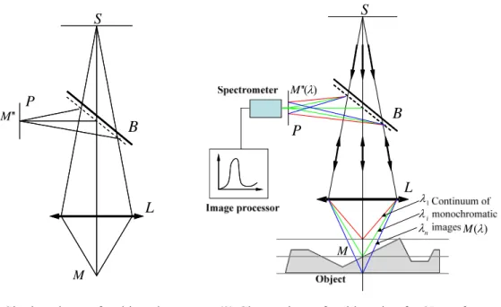
Figure 1-6 (1) describes a basic confocal imaging configuration as a single point viewing system. The point source S is imaged by the objective lens L on the object point M .The retro-diffused light passes back through L and is then directed towards the detector by a beam splitter B . The diaphragm P located at the image of M given by L stops light coming from all points except M .
The altitude (z coordinate) of each point of the surface can be acquired by dynamic focusing, in other terms, by moving some mechanical part along z axis. This operation is very inconvenient in practices. An alternative approach is to extend the z axis by stretching the axial chromatism and working with a polychromatic point source (the most used, for example a white light source). With a univocal color coding to index the different wavelengths, the confocal system turns to a single segment view system, which is the basic idea of the chromatic confocal imaging system. The setup of a classical chromatic confocal imaging system is shown in figure 1-6 (2).
Practically, a white source is imaged by an objective lens with extended axial chromatism on a series of monochromatic point images in the measurement space. When the measured sample intercepts the measurement space at point M , a single of the monochromatic point images is focalized at M . Due to the confocal configuration, only the wavelength λM will pass through the spatial filter with high efficiency, all other wavelength will be out of focus.
'' M M S P L B S L B M P ''( ) M λ 1 λ i λ n λ M( )λ
(1) Single point confocal imaging (2) Chromatic confocal imaging for 3D surface Figure 1-6: Working principle of chromatic confocal imaging system
In general, the confocal imaging principle yields an excellent spatial resolution regardless of ambient illumination. The chromatic coding ensures that measurement is insensitive to reflectivity variations in the sample and allows working with all types of materials. The chromatic confocal imaging sensor can provide high performance in micro-measurement domains.
(2).
Modeling of the chromatic confocal imaging system
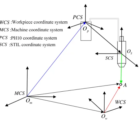
The sensor based on chromatic confocal imaging system implemented in our research works are STIL sensor [Sti], The STIL sensor is composed of a CHR controller with an optical pen. The STIL sensor is a 1D sensor. It can only capture the altitude information (z coordinate) of each point. It hence needs (x, y) scanning to reconstruct its view field. Generally, this operation is achieved by mounting the STIL sensor onto the CMM platform. The x-, y-coordinates are acquired by CMM system. Figure 1-7 specifies the model of the STIL sensing system based on CMM platform.
There are four coordinate systems in the sensing system, as shown in figure 1-7. Machine coordinate system (MCS) is associated with the CMM machine. PH10 coordinate system (PCS) is the coordinate system attached with the PH10 header by which the STIL sensor is mounted on the CMM arm. The STIL coordinate system (SCS) is the coordinate system of the STIL sensor and the workpiece coordinate system (WCS) is the part design coordinate system. The SCS and PCS conform the
same three axes directions. m O p O S O w O A WCS MCS PCS SCS WCS MCS PCS SCS
Figure 1-7: Modeling of the STIL sensor mounted on CMM platform
Considering a point A on object surface, the position vector of A can be represented in WCS, and also can be represented in SCS, Therefore, we can get the following equations:
w m m w
O A=O A O O− (1-13)
m m p p s s
O A=O O +O O +O A (1-14)
Where, O Om p is a translation vector between the PCS and MCS. O Op s is a
vector to record the position of the sensor in PCS. When the sensor is fixed on the PH10, O Op s should be known. O As is the coordinates of A in SCS. The z
coordinate of O As can be acquired by the sensor and the coordinates along x and y
axes can be acquired from the CMM. O Om w is the translation vector between MCS
and WCS.
Combining the equations (1-10) and (1-11), we can finally obtain:
w m p p s s m w
O A=O O +O O +O A O O− (1-15)
From the view of coordinate transformation, the equation (1-15) can be represented as:
w s
O A= ⋅R O A T+ (1-16)
Where, R and T are the rotation matrix and translation matrix from the SCS to the WCS. When the system is setup, all the parameters can be acquired by a calibration process.
(3).
Calibration of the chromatic confocal imaging system
The chromatic confocal imaging sensor used in our experiments is STIL sensor, which is a 1D sensor used in micro-domain with very high resolution (about 0.06 μm). However, the resolution of the CMM on z-axis is only 0.5μm, which is much higher than the STIL resolution. Therefore, during each measurement process, the x-y plane of the CMM has to be fixed to an unchangeable z-value. Otherwise, the resolution of the results will lose greatly.
The calibration process is used to calculate the rotation matrix and translation matrix in equation (1-16). Unlike the contact probing or laser scanning system, the STIL sensor does its position and orientation calibration in two separate ways [Cos07].
The position calibration has the similar strategy with the probing sensors. an artifact should be selected properly considering the micro application nature of the STIL sensor. If the classical sphere is used, the measurement of a small region of the sphere may be not interesting enough to evaluate the spherical center. Instead, we use a facet sphere (shown as figure 1-8 (1)) by measuring the three planar facets to determine the center position of the sphere for the position calibration.
The orientation calibration is used to determine the orientation of the STIL sensor when doing the measurement tasks. For this purpose, two thin films with pre-known thickness values are used as shown in figure 1-8 (2). Assuming the STIL measurement orientation is along the direction z (also 21 z ), the orientation angle between the
measurement orientation and the plummet line can be computed as: arccos( ) 1 2 b a z z θ = − − (1-17)
Where, a and b are the thickness of the two films, which are known before calibration.
Here, we must note that when the orientation of the STIL sensor changes, the orientation calibration has to be done again for correct measurement.
θ z1 θ z2
a b
(1) Facet sphere for position calibration (2) Sketch for orientation calibration Figure 1-8: Calibration of the STIL sensor
1.3. Multisensor integration in coordinate metrology
Besides the mentioned three data acquisition techniques, there are also many methods widely employed for surface digitizing, some of them are represented in figure 1-1. These methods have distinct merits and demerits [NYH97] and hence have their special application ranges. With only one sensor, it could be very difficult to satisfy all the requirements of the ever-increasing complexities of modern data acquisition. The multisensor data fusion methods provide effective solutions to that problem. With multisensor methods, the particular features of a workpiece can be digitized by the most suitable sensor and the small uncertainty can be used to correct data from other sensors which exhibit relevant systematic error but have a wider field of view or application range [WJS09]. Thereby, the merits of each integrated sensor can be fully utilized and their demerits can also be avoided to improve the acquisition performance of the whole system.1.3.1. Multisensor configuration
An important issue for multisensor measurement is how to integrate the multiple sensors onto a common measurement platform (e.g. CMM). The physical sensor configurations can be roughly classified into three categories [Dur88, WJS09] as shown in figure 1-9.
acquired data can be combined to give more complete information of the measured object. An example of this configuration is the fusion of images captured with different illumination series to achieve images with higher contrast [HL03].
Competitive system is that when the sensors are configured as independent to measure the same feature in order to reduce the measurement uncertainty.
Cooperative configuration uses the information provided by two or more independent inhomogeneous sensors to derive data that would not be available from the sensor individually. The particular examples mentioned this kind of sensors configuration are related to multisensor integrated on the CMM platform and use the data acquired by an optical sensor to guide the tactile probing measurement [CBV01, NYH97].
Sensor 3 Sensor 4 Data Fusion
(1) Complementary (2) Competitive (3) Cooperative Figure 1-9: Three sensors configurations in multisensor systems
1.3.2. Multisensor data fusion
In applications, a particular multisensor measurement system may be configured as the combination of the two or more models to fulfill the complete measurement tasks. The data acquired by the multiple sensors, dependently or independently, are
other. Thereby, how to merge the multiple data models and process to extract the geometrical features should be one of the most important stages for multisensor measurement. There is a great deal of issues that should be considered properly for data processing in order to achieve the multisensor integration. Generally, the process of the multisensor data fusion should comprise the following procedures:
(a) Pre-processing: the raw data acquired from multiple sensors are typically preprocessed to improve their qualities, such as denoising, filtering, etc. After pre processing, the data are more reliable for further processing. The pre-processing in multisensor data fusion should also include the data format conversion when it is necessary.
(b) Registration: every employed sensor has its own coordinate system which is usually different from each other. The measured data captured by respective sensor represented in its own coordinate system should be aligned and merged into a common coordinate system so as to represent the model completely. Moreover, in the recognition and position stages prior to the shape inspection, the digitized data from unfixed rigid objects also need to be registered with an idealized geometric model [BM92]. Therefore, registration is one of the most critical issues and decisive phases for data fusion and data processing and it hence should be taken into account.
(c) Fusion: data fusion procedure is performed to decide which data should be merged into the final data set, how to extract the useful information and how to handle the redundant data. The methods for data fusion should belong to one the following three clusters: estimation, inference, fuzzy or neural methods [WJS09]. Estimation methods, which include least square analysis [BRM92], weighted average [TGC04], Kalman filtering based methods [HQC09], etc., are suitable to analyze the measurement systems in which various results are acquired for the same measurand or for a regression plot are combined. Inference methods, like Bayesian probability theory [Pun99] are usually used to evaluate the measurement uncertainty.
1.3.3. Related works in multisensor integration
Comprehensive research activities have been addressed in multisensor based data acquisition. Multisensor fusion technique is an active issue in many applications, e.g. Robotics [ATS04], pattern recognition [GAG09], medicine [DVD02], non-destructive testing [KZD05], geo-sciences [MWW09], military reconnaissance and surveillance
[GPL04], etc. In the following sections, comprehensive research activities related to dimensional metrology and reverse engineering are surveyed.
(1).
Homogeneous optical sensors integration
Measurement tasks in many applications require high quality data. The necessary quality is often achieved by applying data fusion methods across sensors, which is also called multi-model analysis. The integrated homogeneous sensors in such systems usually are cameras, laser scanners, or other optical sensors. Moreover, a series of images captured by the same sensor (named virtual sensors [WJS09]) also can be classified into this category.
One classical example of this integration setup is when applying the shape from shading technique. The setup consists of different illumination sources and a fixed camera. The camera captures a series of grayscale images with different illuminations. With the gradients analysis in these images, the height map of the object can be derived [Fra08, SRM06].
Another typical example is the multi-station photogrammetry network which integrated with several homogenous cameras. After calibration process [BA00] of each camera, each observation can be captured with several images simultaneously. These images finally can be registered to obtain a final global point cloud of the objects. Similar systems can be referred in [ALT05, SNK02, LPZ06].
For the shape measurement with complex structures, because the high accuracy of fringe projection systems [LLZ07], some researchers used the fringe projection sensor to replace the camera and constructed the measurement setup integrated with multi fringe projection sensors. Examples can be found in [WWH08, PZT02].
Some researchers, however, don’t combine multiple sensors to capture multiple data. Instead, they use a single optical sensor to digitize the object several times to obtain a series of point data with different positions, focus depths or view orientations. More detail information of the object can then be extracted from these point data. Due to its economic cost cheap (only one sensor is required) and flexibility, these systems are quite widely researched and implemented.
C. Souzani, et al. [MTL06] developed a laser scanner self-guidance measurement system. In their system, the object is first scanned to generate the initial point data
using the same scanner.
For the objects which are beyond the measurement area of the sensor or too complex to be captured in one single measurement, Using one sensor to capture a series of partial views from different sensor positions and fusing them together is an effective solution. Similar systems are also mentioned in [Wil01, PZT02, XZJ06]. The methods in which the same feature is captured by a single camera from different positions to enhance the image quality are also discussed in [PK06, Pie03].
(2).
Contact and optical multisensor integration
In modern dimensional metrology or reverse engineering, the increasing requirements in terms of flexibility and automation of the whole digitization process result in a great deal of research efforts on cooperative integration of inhomogeneous sensors. The sensors implemented in such systems mostly are mechanical probes and optical sensors [WJS09].
The optical sensors can be a simple video-camera, or a laser scanner, which acquires the global shape information and provides the guidance information to drive the CMM execute the local exploration with a more precise tactile probe [ZAB09]. In such systems, the strengths of the two kinds of sensors, i.e. the ability of an optical sensor to quickly generate the global information and the ability of a contact probe to obtain higher accurate measurement data, can be ensured at the same time. There have been considerable researches on the cooperative sensor integration.
Chan, et al. [CBV01] developed a multisensor system integrating a CCD camera and a tactile probe on CMM platform for reverse engineering. The two sensors are fixed on the CMM arm together. The images captured by the CCD camera are processed by neural network based method to provide the geometric data which can be used for planning the probing path of the tactile sensor. The CCD images play the role of the CAD model like in CAD model based inspection planning systems [ZWW06].
Similarly, Carbone, et al. [CCS01] proposed a method to combine a stereo vision system and a scanning touch probe. In their method, the 3D vision system is performed to acquire a number of clouds of points which are fused to approximate the initial CAD model and to guide the CMM programming of the touch probe. The touch points data are then import to the CAD environment to produce the final, accurate
CAD model. The approach mentioned in [CL97] uses the similar way for reverse engineering.
Nashman et al [NYH97] integrated a vision system and a touch probe for dimensional metrology purpose. In their method, The Vision camera is fixed on the CMM table and the touch probe is mounted on the CMM arm with three translation degree-of-freedom. The workpiece is located in the view field of the camera. The images captured by vision camera are used for the workpiece positioning. With comparison of the image data and the data generated by the machine scales and the probe, the position of the probe to the interested features are computed to guide the path generation of the tactile probe. The tactile measurement can provide the final inspection data.
Menq, et al. [SHM00, SHM01] presented a cooperative sensor integration system that fused a vision system and a touch probe for coordinate metrology. The objects are first scanned by the vision system to recognize the global information. Due to the occlusion of the vision system, some regions may be not able to be digitized. In their method, they estimated the unknown regions from the vision data to guide the touch probe to supplement the missing data. The regions that require higher accuracy are also probed again by the touch sensor. The multisensor based inspection planning algorithms were researched based on information integration.
More recently, Huang and Qian [HQ07] developed an approach to combine a laser scanner and a touch probe dynamically. A workpiece is first scanned by the laser scanner to capture the overall shape. It is the probed by a touch sensor where the probing positions are determined dynamically to reduce the measurement uncertainty according to the scanning data. They use the Kalman filtering to fuse the data together and to incrementally update the surface model based on the dynamic probed points.
In the methods demonstrated in [ASG04, EC01, JOM06], a laser scanner is used to detect the large point cloud data files required to define freeform surfaces, whereas a CMM touch probe is used to precisely define the boundary of bounding contours. Both sensors are mounted on the CMM arm. Generally, the objects need several scans with different views by the laser scanner to acquire complete point data. Multisensor systems in which, other sensors, like conoprobe [CWL03] or construct lighting sensor [XWZ05] are also mentioned in literatures. The digitizing errors are also analyzed in [EC01]. In some papers, the multisensor calibration problem has been researched to
reduce the measurement uncertainties [HQ07, HQC09 and SHM00].
(3).
Inhomogeneous optical sensors integration
Like the optical/contact sensors integration, the multiple optical sensors with different principles can be well combined by cooperative integration. Hence the different resolutions and multi-scales measurement can be ensured in a single system with the inhomogeneous sensors integration.
In such systems, the lower resolution sensors (e.g. conventional camera) are usually used to capture the global information. Then, a data analysis phase follows to evaluate the integrity of the measurement data. If there is not enough information, further local measurements with higher resolution sensors are required in which the position of the local measurement regions, the configuration of the sensors are often derived from the global information. The final result data are updated after combining each additional measurement datum until the measurement tasks are fulfilled [WJS09]. The system developed by SoKolov, et al. [SKT05] combined a confocal sensor and a scanning probe sensor for nano coordinate metrology. The feasibility of combining an SPM (Scanning Probe Microscope) with an optical interference microscope in a single measurement is demonstrated in [TDK04]. Weckenmann, et al [WN03] combined a white light interferometer sensor and a fringe projection sensor to measure the wear of cutting tools.
Some systems have also mentioned the integration methods to combine several optical sensors for the complementary configuration [RRT01, SPM03].
Other multisensor systems applied to different purposes in dimensional metrology and reverse engineering are surveyed in [WJS09] and dimensional metrology for freeform shape measurements are well surveyed in [SDS07].
(4). Commercial
Systems
Multisensor CMMs use a combination of several sensors to provide higher precise or larger ranges of the measurements. Many CMM manufacturers, like, Mahr, Hexagon, Werth Messtechnik, Zeiss, etc. [CN04], can provide the multisensor solutions. Most of these solutions combine the optical sensors with a tactile probe in a cooperative configuration, which yield the following advantages.
can guide the more precise sensors automatically.
(b) The inhomogeneous sensors capture the information that would be not available from a single sensor, which provides more details about the object. The holistic measurements can be achieved.
Some commercial systems integrate the measurement vision system, different optical and contact sensors, but also can include the sensors based on computed tomography, fiber probe [CN04, CZ08, Myc08]. However, the methods combining the different sensors in these systems are usually not published due to commercial purposes. Additionally, multisensor systems based on tracker sensors [Met08], inerferometry or photogrammetry [GFM08] etc. are also available.
(5).
Integration within a PLM context
The measurement system is not isolated and should be integrated with other activities in the context of PLM (Product Lifecycle Management). It is also an important issue to embed the measurement activity into the integrated manufacturing process. The reverse engineering should also consider the integration problem because the point data should reconstruct the CAD model which needs to satisfy the design intention and specifications. There are also considerable research works trying to achieve the system integration of measurement systems with CAD/CAM systems or measurement execution systems. We will survey the related research literature in this section.
The most common solution for the system integration is based on interface standards in which the data in each respective system which would be exchanged with other systems are specified with standard file formats. The systems parse and derive the useful information from these standard data. Many standards and neutral files are published for these purposes, like STEP (Standard for the Exchange of Product Model Data) [Step], DMIS (Dimensional Measuring Interface Standard) [Dmis], DML (Dimensional Markup Language) [Dml], I++DME (Inspection plus plus Dimensional Measurement Equipments) [Nist] etc. The figure 1-10 shows the general interfaces in the dimensional metrology systems proposed by NIST [Hor05].
![Figure 1-10: Interface standards in dimensional metrology systems [Hor05]](https://thumb-eu.123doks.com/thumbv2/123doknet/14528079.723160/43.892.179.714.112.474/figure-interface-standards-dimensional-metrology-systems-hor.webp)