ttH, H en WW avec analysis at ATLAS, LHC and very low energy electron studies of 2004 combined test beam

HAL Id: tel-00366852

https://tel.archives-ouvertes.fr/tel-00366852

Submitted on 9 Mar 2009

HAL is a multi-disciplinary open access archive for the deposit and dissemination of sci-entific research documents, whether they are pub-lished or not. The documents may come from teaching and research institutions in France or abroad, or from public or private research centers.

L’archive ouverte pluridisciplinaire HAL, est destinée au dépôt et à la diffusion de documents scientifiques de niveau recherche, publiés ou non, émanant des établissements d’enseignement et de recherche français ou étrangers, des laboratoires publics ou privés.

H. Zhang

To cite this version:

H. Zhang. ttH, H en WW avec analysis at ATLAS, LHC and very low energy electron studies of 2004 combined test beam. Physics [physics]. Université de la Méditerranée - Aix-Marseille II, 2008. English. �tel-00366852�

UNIVERSIT´E DE LA M´EDITERRAN´EE AIX-MARSEILLE II

FACULT´E DES SCIENCES DE LUMINY

163 Avenue de Luminy 13288 MARSEILLE Cedex 09

TH`ESE DE DOCTORAT

Sp´ecialit´e : Physique math´ematique, physique des particules et mod´elisation dans le cadre d’une co-tutelle de th`ese entre:

Institute of High Energy Physics, Chinese Academy of Sciences, China Centre de Physique des Particules de Marseille, France

pr´esent´ee par Huaqiao ZHANG

en vue d’obtenir le grade de docteur de l’Universit´e de la M´editerran´ee

Analyse ttH, H → W W

(∗)

avec ATLAS au LHC et

´

Etude des ´

Electron `

a Tr`

es Basses ´

Energie dans le

Test Faisceau Combin´

e 2004

ttH, H → W W(∗) _{analysis at ATLAS, LHC}

and Very Low Energy electron studies of 2004 combined test beam

Soutenue le 10 Juin 2008 devant le jury compos´e de : M. GuoMing Chen

M. YuanNing Gao Pr´esident

M. Liang Han M. Yi Jiang

M. Shan Jin Directeur de th`ese IHEP

M. YaJun Mao

M. Emmanuel Monnier Directeur de th`ese CPPM M. Qun OuYang

1 Preface 1

1.1 Standard Model and Higgs . . . 1

1.1.1 Symmetry in particle physics . . . 3

1.1.2 Higgs mechanism . . . 4

1.1.3 Yukawa Coupling of top quark and Higgs . . . 7

1.1.4 Quantum Chromo Dynamics(QCD) . . . 7

1.1.5 Challenge of the Standard Model . . . 8

1.2 Physics at TeV proton-proton collision . . . 10

1.2.1 QCD processes . . . 10

1.2.2 Physics of electroweak gauge bosons . . . 10

1.2.3 B physics . . . 10

1.2.4 Heavy quarks and leptons . . . 11

1.2.5 Higgs Physics . . . 11

1.2.6 SUSY and Physics beyond Standard Model . . . 12

1.3 Motivations of thesis . . . 12

1.3.1 Research background . . . 12

1.3.2 Historical status of the study . . . 13

1.3.3 Motivation of the study . . . 15

1.3.4 Structure of this thesis . . . 18

2 Introduction of LHC and ATLAS 21 2.1 The Large Hardron Collider(LHC) . . . 21

2.2 The ATLAS detector . . . 24

2.2.1 ATLAS detector requirements to fulfill the physics goals . . . 24

2.2.2 ATLAS designed performance . . . 25

2.2.3 ATLAS overview . . . 26

2.3 Data transportation, storage and analysis of ATLAS . . . 48

3 Analysis of t¯_{tH(H → W W}(∗)_{) production channel 53} 3.1 Introduction . . . 54

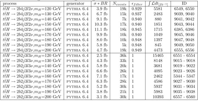
3.2 Generation of Monte Carlo Sample . . . 57

3.2.1 Signal Generation . . . 57

3.2.2 Generation of Background Samples . . . 58

3.2.3 Monte Carlo simulation and reconstruction . . . 59

3.3 Trigger study . . . 60 i

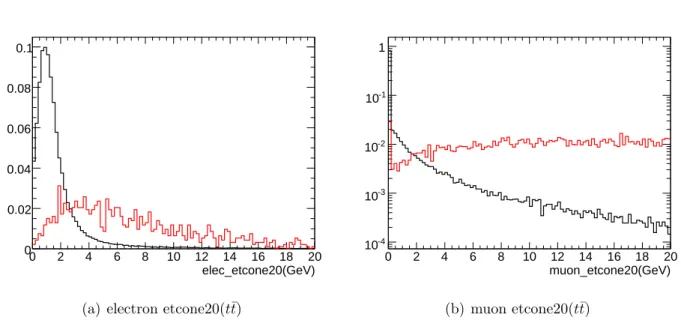
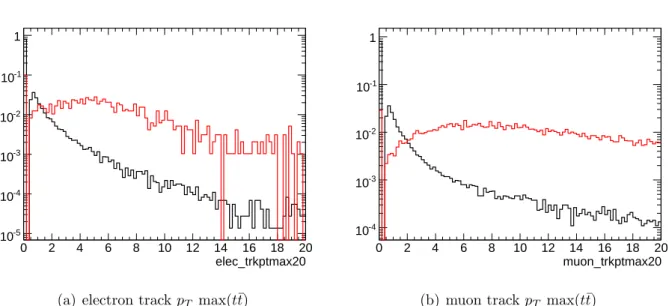
3.5 Lepton Isolation . . . 68

3.6 t¯_{tH, H → W W}(∗) _{two lepton final states analysis . . . 70}

3.6.1 Event selection and background suppression . . . 72

3.6.2 Optimization of isolation . . . 74

3.7 t¯_{tH, H → W W}(∗) _{three leptons final state analysis . . . 75}

3.7.1 Event selection and background suppression . . . 76

3.8 Pileup study . . . 77

3.8.1 Pileup impact on lepton ID efficiency . . . 77

3.8.2 Pileup impact on jets . . . 78

3.8.3 Pileup impact on lepton isolation . . . 78

3.8.4 Pileup impact on signal and background . . . 79

3.9 Systematic uncertainties . . . 80

3.9.1 Luminosity . . . 81

3.9.2 Theoretical uncertainties . . . 81

3.9.3 Detector performance uncertainties . . . 83

3.9.4 Systematic uncertainty on Monte Carlo based predictions . . . 87

3.10 Top quark and Higgs boson Yukawa Coupling measurement . . . 88

3.10.1 Significance of signal . . . 88

3.10.2 Precision of σt¯tH ∗ BrH→W W measurement at 30 fb−1 . . . 88

3.10.3 Precision of gt measurement at 30 fb−1 . . . 89

3.11 Conclusion and discussion . . . 90

4 Combined Test Beam description 93 4.1 Introduction . . . 93

4.2 ATLAS Test Beam detector setup . . . 94

4.3 The test beam line . . . 96

4.4 Beamline instrumentation . . . 96

4.4.1 Cerenkov counters . . . 96ˇ 4.4.2 Beam Chambers . . . 99

4.4.3 Scintillators . . . 99

4.4.4 Trigger and readout . . . 100

4.5 Energy Reconstruction in Liquid Argon . . . 100

4.5.1 Energy reconstruction of single cell . . . 101

4.5.2 Performance of electron energy reconstruction in EM calorimeter . . 107

5 Combined Test Beam data analysis 111 5.1 CTB VLE electron energy linearity studies . . . 112

5.1.1 VLE electron selection criteria . . . 112

5.1.2 Reconstruction of single VLE electron true energy . . . 114

5.1.3 Calculation of VLE electron EBCmeasured/Ereco . . . 122

5.1.4 Linearity of VLE electron LAr measured energy . . . 122

5.2.4 Electron energy calibration . . . 127 5.3 Conclusion and discussion . . . 132

6 Summary and prospects 135

bibliography 137

Preface

Contents

1.1 Standard Model and Higgs . . . 1

1.1.1 Symmetry in particle physics . . . 3

1.1.2 Higgs mechanism . . . 4

1.1.3 Yukawa Coupling of top quark and Higgs . . . 7

1.1.4 Quantum Chromo Dynamics(QCD) . . . 7

1.1.5 Challenge of the Standard Model . . . 8

1.2 Physics at TeV proton-proton collision . . . 10

1.2.1 QCD processes . . . 10

1.2.2 Physics of electroweak gauge bosons . . . 10

1.2.3 B physics . . . 10

1.2.4 Heavy quarks and leptons . . . 11

1.2.5 Higgs Physics . . . 11

1.2.6 SUSY and Physics beyond Standard Model . . . 12

1.3 Motivations of thesis . . . 12

1.3.1 Research background . . . 12

1.3.2 Historical status of the study . . . 13

1.3.3 Motivation of the study . . . 15

1.3.4 Structure of this thesis . . . 18

1.1

Standard Model and Higgs

The Standard Model is the most accurate theory that describe the fundamental structure of mater and interactions. In this model, the fundamental constituents of mater are quarks and leptons, and the interaction are linked to carrier particles called bosons. Quarks and

present knowledge, all of them are point like particles. No experimental evidence of finer structure was found. These leptons and quarks are divided into three generations, each generation has four members, each member of same generation has different charge and mass. For these leptons and quarks, there are corresponding particles. These anti-particles have same masses, but opposite sign of all other quantum numbers compared to the corresponding particles [1, 2]. There are upper, charm and top quarks, whose charges

are (−23). There are also down, strange and bottom quarks, whose charges are (−

1

3).

Leptons are of two kinds. One set of them like electron, muon and tau particles, with a charge (−1), while the other set of them are neutral neutrinos, corresponding to each type of lepton. Figure 1.1 is the schematic plots of the fundamental particle classification.

Z

Z 0 91187 0 ₀ 8 Gluon Name # of color charges Mass in MeV 0 _ + _ 0

g

0 0 Photon 0

γ

Symbol 3 ~5 3 3 Down

d

-1/3 Strange -1/3 -1/3 Electric charge

s

+ ~175 ~4500 +2/3 3

t

Top

u

3 Up ~5 +2/3 3

c

Charm ~1350 ~180000 Bottom 0 0 0 -1 -1 -1 Electron neutrino Muon neutrino neutrino Tau

Electron Muon Tau

e

ν

0 0 0 0 0 0

e

<10

ν

µ

<0.27

ν

τ

µ

τ

< 23 0.51 105.7 Leptons -6 1777.0

b

+2/3 Electromagnetic

The Three Generations of Matter Force Carriers

Interactions Strong Interactions Interactions Weak Vector Bosons Fermions Quarks 0

W

W 1 80360

Figure 1.1: Categories of fundamental particles

There are four different interactions in nature: Strong force, Electromagnetism, Weak force and Gravity. The propagators of these interactions are the names of force

carrier particles. They are Gluon for strong force, photon for electromagnetism, W±_{, Z}0

for weak force and graviton for gravity. The first three kinds of force carriers all have spin one bosons and have been found experimentally, while the fourth has not been found until now and the theoretical prediction is spin two. The unique particle, Higgs, which give masses to these fundamental particles, does not belong to any category of particles described above. The properties of the four force carriers are listed in table 1.1.

electromagnetism weak interaction strong interaction gravity

Sources charge weak charge color mass

Intensity e2 ~c≃ 1 137 ( mpc ~ )2 G~c∼ 10 −5 g2 ~c ≃ 10 Gm2 p ~c ∼ 10 −38

Force range Long range short range short range long range

(m) ∞ ∼ 10−18 ₁₀−15 _∞

photon W±_{, Z}0 _{Gluon Graviton(in theory)}

propagator γ W± ,Z0 _{g G} JP ₁− 1? ₁− 2+ MW± = 80.4 Mass(GeV) Mγ= 0 MZ0= 91.2 Mg= 0 MG= 0

Electro-Weak Dynamics Quantum Chromodynamics Geometric Dynamics

Theories

(EW) (QCD) (General relativity)

Table 1.1: Properties of four interactions

Since the last 70 years, physicists are trying to unify these four interactions. Varies attempts have been tried in different directions. But the most successful ones belong to

Gauge Theory. Electro-Weak theory is SU (2)L×U(1)Y Gauge Theory. Quantum Chromo

Dynamics is SUc(3) Gauge Theory. These two theories constitute the Standard Model,

which is a SUc(3) × SU(2)L× U(1)Y Gauge Theory. Higgs particle is a scalar which

gives masses to gauge bosons through the Higgs mechanism and gives mass to fermions by Yukawa Coupling [3].

1.1.1

Symmetry in particle physics

The phenomena of symmetry have existed since time begins. Such as day after day, year after year. Also phenomena of symmetry are very common in our lives. Such as sun in the sky, Si He Yuan in Beijing, the rolling wheel. Symmetry picture is popular. Such as most people prefer symmetrical plots, symmetrical face. So, in our lives, people are likely using symmetry approach to describe things.

Although the symmetry is beautiful, the symmetry breaking makes people more profound understand the nature of things. Like the symmetry of sunrise, let people believe that the earth is the center of the universe, because it is in people’s love of symmetry, but those strange tracks and movements of planets and stars destroy the symmetry of Earth as the center, so that people come to the awareness of sun as the center, and now the knowledge of galaxies and even the knowledge of the entire universe.

In particle physics, symmetry and symmetry breaking are also ubiquitous. Field theories are used to describe the dynamics of particle physics. According to Noether’s theorem, any differentiable symmetry of the action of a physical system has a corre-sponding conservation law. The action of a physical system is an integral of a so-called Lagrangian function, from which the system’s behavior can be determined by the principle of least action. Thus, the invariance of time-space transformation accounts for energy and linear momentum conservation of this system. The invariance of Lorentz transformation accounts for angular conservation. Gauge transformation invariance is one of the basic transformations of field.

compo-nent of φσ(x) with the transformation of:

φσ(x) → φ′σ(x) = exp[−iθαTσρα]φρ(x) . (1.1)

of which Tα _{matrices are the generators of gauge group G. There is one conserved current}

for every generator. This group is non Abelian. Their commutation relations are:

[Tα_{, T}β_{] = if}αβγ_Tγ _(1.2)

Where fαβγ _{are the group structure constants of SU(3). The transformation satisfy}

the form described above is called gauge transformation. If the Group Parameters θα _is

time-space independent constant, it is a global gauge transformation. If θα _{is time-space}

dependent function of θα_{(x), it is a local gauge transformation.}

Gauge Field: Unfortunately, the transformations of normal Lagrangian can not

pass the derivatives of gauge invariance if θα_{(x) is time-space dependent. In order to get}

a local gauge invariant symmetry, the gauge transformation Lagrangian density can be written as: L = −1 4F α µ,νFµ,ν,α . (1.3) Of witch Fα

µ,ν is the strength of gauge field, and it is defined as:

F_µ,να = ∂µAαν − ∂νAαµ+ gfαβγAβµAγν , (1.4)

This Lagrangian describes particles of spin 1, such as photon, intermediate bosons, gluons. And g is the coupling constant - a quantity defining the strength of an interaction.

However, If mass term of 1

2M

2

AAµAµ added in this Lagrangian, it is not invariant with

the gauge transformation of equation 1.1. Since there is no way to add the square term

of field Aα

µ(x), it means that all the gauge bosons that described by this Lagrangian are

massless. While in fact, W±_{, Z}0 _{intermediate bosons have masses ∼ 80 − 90GeV . So, the}

Higgs mechanism described in the following section was introduced to solve this problem.

1.1.2

Higgs mechanism

Due to the constraint of gauge invariance, the Lagrangian of gauge field can not contain square term of the field. It results that gauge particles are massless in this theory. Therefor this Gauge Theory is not the exact description of intermediate bosons since they have masses. To solve this problem, the Higgs mechanism has been introduced.

1.1.2.1 Spontaneous symmetry breaking and Goldstone particles

Consider a simple real scaler field φ(x) with a usual Lagrangian:

L = 1₂∂µφ∂µ_{φ − V (φ), V (φ) =} 1

2µ

2_φ2₊ 1

4λφ

4 _{, (1.5)}

It is invariant under the internal space reflection transformation of φ(x) → −φ(x)

it is the the Higgs field. Due to the potential bound condition, the self coupling coefficient λ must be greater than zero. So, the potential V (φ) is symmetrical of its internal space. But the minimum V (φ) is not any more at φ(x)=0(see figure 1.2).

Figure 1.2: The potential V of the Higgs field φ

The vacuum expectation value (vev) of φ2 _{is defined as < 0|φ}2_{|0 >≡ φ}2

0 = −µ

2

λ ≡ v

2_. In order to interpret correctly the theory, we expand the Lagrangian around one of the minimal v by a translation transformation of φ(x):

φ(x) = φ′(x) + v , (1.6)

Then, the Lagrangian of Higgs field becomes:

Lφ′ = 1 2∂µφ′∂ µ φ′ + µ2φ′2− λvφ′3− 1 4φ′ 4 _{, (1.7)}

This is a scalar field with a real mass of p−2µ2 _{instead of virtual mass i}p−µ2

before transformation. And it has cubic and fourth order self coupling terms. So, this Lagrangian is not invariant under the reflection transformation of its internal space. Gold-stone theorem indicates that: for each generator of the symmetry that is broken, there is one massless(light if the symmetry was not exact) scalar particle - called a Goldstone

boson. For O(N ) rotation group, there are 1_{2n(n − 1) generators, of which} 1_{2(n − 1)(n − 2)}

generators are vacuum invariant transformations, and (n − 1) generators of the symmetry that is broken. So, there exist (n − 1) massless Goldstone particles. In gauge theory, the Goldstone bosons are ”eaten” by the gauge bosons. The latter become massive and their new, longitudinal polarization is provided by the Goldstone boson.

1.1.2.2 Higgs mechanism

In Electro-Weak theory, the Lagrangian of free boson can be written as:

Lboson = − 1 4W α µνWαµν− 1 4BµνB µν _{, (1.8)} of which: W_µ,να = ∂µWνα− ∂νWµα+ gfαβγWµβWνγ , (1.9) Bµ,ν = ∂µBν − ∂νBµ , (1.10) Wα

µ,ν,α = 1, 2, 3 are the field strength of SU (2)L vector bosons. Bµ,ν is the field

strength of U (1)Y vector boson. Together with the Lagrangian of Higgs scalar:

LS = (Dµφ)†(Dµφ) − µ2φ†φ − λ(φ†φ)2 , (1.11) of which Dµ = ∂µ− ig2 τα 2 W α µ − ig1 1 2Bµ , (1.12)

It already includes the interaction term between Higgs field and SU (2)L,U (1)Y vector

field. Expand Higgs field according to its four compartments, after the vev calculation and local gauge transformation, we define:

W± = _√1 2(W 1 ∓ iW2) (1.13) Zµ = g2Wµ3− g1Bµ pg2 1 + g22 (1.14) Aµ = g2Wµ3+ g1Bµ pg2 1 + g22 (1.15)

After these calculation of Lboson+ LS, and from the square terms of W±, Z, A fields,

one can obtain the mass term for each particle as:

M_W± = 1 2vg2, MZ = 1 2v q g2 1 + g22, MA= 0 , (1.16)

Now, in SU (2)L+ U (1)Y → U(1)Q spontaneous symmetry breaking gauge theory,

the Goldstone bosons are ”eaten” by the gauge bosons W± _{and Z. The gauge bosons}

longitudinal polarization is provided by the Goldstone bosons, corresponding to the bro-ken generators, which gives the gauge bosons masses and the associated necessary third

polarization degree of freedom. Since U (1)Q does not break its symmetry, photon remains

1.1.3

Yukawa Coupling of top quark and Higgs

Under the framework of Standard Model, fermions obtain masses from Yukawa Coupling with Higgs. The Lagrangian of fermions can be written as:

LF ermion = − X F,σ gF,σ √ 2 ³ ψL FφψRF,σ+ ψF,σR φψfL ´ (1.17) of which g is the Yukawa Coupling constant. L and R denote left hand and right hand Dirac wave function respectively. F denotes the generations of fermions and σ denotes the spin. After similar transformations and simplifications as section 1.1.2.2, one gets: LY ukawa = −(1 + h v) X F ¡mFψFψF ¢ (1.18) So, the mass term of fermions are:

mF =

vgF

√

2 (1.19)

of which, gF is the corresponding fermion to Higgs Yukawa Coupling constant. v is

the Higgs field vacuum expectation value, which is about 246 GeV. Equation 1.19 shows

that gF is independent of Higgs mass, and proportional to the mass of its corresponding

fermion. In Standard Model. The heaviest quark is top, with a mass about 172 GeV. Which means that top Yukawa Coupling constant is the largest one, about one, and therefor will be most probably the first Yukawa Coupling constant that could be measured experimentally.

1.1.4

Quantum Chromo Dynamics(QCD)

Quantum Chromo Dynamics is a non-abelian gauge field theory of the strong interaction compartment of SU (3) × SU(2) × U(1) Standard Model. It describes the dynamics of colored quarks and gluons. A quark of special flavor has three different color states, while gluons have 8 possible color states. Hadrons are colorless combination of quarks, anti-quarks and gluons. The dynamics of the anti-quarks and gluons are controlled by the quantum chromo dynamics Lagrangian. The gauge invariant QCD Lagrangian can be written up to the gauge fixing terms as:

LQCD = − 1 4F (a) µν F(a)µν+ i X q ¯ ψ_qiγµ(Dµ)ijψjq− X q mqψ¯qiψqi , (1.20) F_µν(a) = ∂µAaν − ∂νAµa− gsfabcAbµAcν , (1.21) (Dµ)ij = δij∂µ+ igs X a λa i,j 2 A a µ , (1.22)

where gs is the QCD coupling constant, fabc are the structure constants of SU(3),

The ψi

q(x) are the 4-component Dirac spinors of each quarks of color i and flavor q. And

Aa

µ(x) are the Yang-Mills gluon fields. QCD has two peculiar properties:

ˆ Asymptotic freedom: which means that in very high-energy reactions, quarks and gluons interact very weakly. This prediction of QCD was first discovered in the early 1970s by David Politzer and by Frank Wilczek and David Gross. For this work they were awarded the 2004 Nobel Prize in Physics.

ˆ Confinement: which means that the force between quarks does not diminish as they are separated. Because of this, it would take an infinite amount of energy to separate two quarks; they are forever bound into hadrons such as the proton and the neutron. Although analytically unproven, confinement is widely believed to be true because it explains the consistent failure of free quark searches, and it is easy to demonstrate in lattice QCD.

There are several methods in QCD calculations, one of them is Perturbative QCD, which is based on the Asymptotic freedom and could be accurate at very high energies. This can be tested with a certain accuracy at TeV energy scale.

1.1.5

Challenge of the Standard Model

The Standard Model is based on quark model and gauge theory. It successes in describing strong interactions, weak interactions and electromagnetism, which provides an internally consistent theory describing interactions between all experimentally observed particles, only the predicted Higgs particle has not yet been found experimentally. SM is one of the greatest achievements of physics in 20th century, and proved to be correct in the recent 30 years of precision experimental tests:

ˆ In 1973, neutral current was predicted and confirmed shortly thereafter, in a neutrino experiment in the Gargamelle bubble chamber at CERN.

ˆ In 1974, the fourth quark -Charm quark- was discovered by Ting and Richter. Which was highlighted by the rapid changes in high-energy physics at that time.

ˆ In 1975, tau lepton was discovered by Perl, which extend leptons to be three gener-ations.

ˆ In 1979, three-jet events were observed at the electron-positron collider at DESY by X.L. Wu and Ting. Which gives the evidence of gluons.

ˆ In 1983, W± _{and Z}0 _{were discovered by Rubbia at SPS, which are the intermediate}

bosons that carrying weak forces.

ˆ During 1990 to 2000, LEP experiments performed precision tests on Standard Model,

including the running αs coupling constant, which proves the asymptotic freedom

predicted by the Standard Model.

Although the Standard Model gives answers to many questions raised in particle physics, and predicts many particles confirmed by experiment. It is still not a complete theory of fundamental interactions and still raised unanswered questions.

ˆ The Standard Model can not be a complete theory, primarily because of its lack of inclusion of the gravity, the fourth known fundamental interaction, but also because of the eighteen numerical parameters (such as masses and coupling constants) that must be put ”by experimental measurement” into the theory rather than being derived from first principles. Of these 18 parameters, a small fraction of them comes from gauge theory, relevant to the symmetry of physics. It needs deeper understanding of these possible symmetries. Other free parameters come from the Higgs field and breaking of symmetry, also need more studies. Higgs particles has not yet been found experimentally, Higgs searching is one of the direct tests of Standard Model.

ˆ Similar as the periodic table of the chemical elements, leptons and quarks have some properties in common. They may have more fundamental bases and structures. High energy physics are approaching a finer structure of mater: the structure of quarks and leptons. Also, the possible structure of force carriers are important research area.

ˆ How to understand the properties of leptons, quarks, force carriers of photon, inter-mediate bosons, gluons, graviton, Higgs and the interactions between them, How to develop a fundamental theory, which can unifies the experimental results and take the Standard Model as proximation. These questions still need a long way to be answered.

ˆ Three generations of leptons and quarks have different properties, but they also have same quantum numbers such as hyper charge and isospin. How to understand the ”generations”, why there are 2 generations of unstable particles. Is there new generations other than these three? All these need further experimental evidence and studies.

ˆ the asymmetry of mater and anti-mater in universe. Scientists predicts that about 14 billion years ago, when universe was born, the mater and anti-mater were gen-erated equally. But now, the observed universe are mostly composed of mater, the missing anti-mater need more studies.

There are great efforts of both theoretical and experimental researches exploring whether the Standard Model could be extended into a complete theory of everything, at

grand energy range. This area of research is often described by the term ”Beyond the Standard Model”. Maybe one day, there will be a ”super standard model” that could solve all these problems of Standard Model, from first principles.

1.2

Physics at TeV proton-proton collision

The Large Hadron Collider (LHC) is a particle accelerator located at CERN. It is a proton proton collider at the designed center of mass energy of 14 TeV. The designed luminosity

is 1034_cm−2_s−1_{. The total reaction cross section at LHC is about 100mb, and the inelastic}

reaction is about 109 _{per second [4]. Under such extreme hard environment, the Higgs}

signal that we are most interested in only has about 10−10 _{of the total production cross}

section. At this new experimental energy scale, there are many interesting physics that can be studied.

1.2.1

QCD processes

QCD processes have the largest production cross section at LHC. There are two main goals of QCD processes studies. One is precision measurement and tests of QCD predictions. Additional constraints to be established by these tests. Such as parton density function in

the proton, or the running strong coupling constant αstested at various energy scales. The

other main goal is that since QCD processes represent a major part of the backgrounds to all other Standard Model processes or new physics, they need to be known precisely to verify the deviations from QCD expectations.

1.2.2

Physics of electroweak gauge bosons

There will be abundant gauge bosons and gauge-boson pairs produced at LHC. Thanks to the high statistics and center of mass energy, we can perform several precision measure-ments at LHC, which will significantly improve the precision achieved at present machines.

Such as the W± _{bosons masses, and the measurement of Triple Gauge Couplings (TGCs).}

Meanwhile, the measurement of these gauge boson production will be important to un-derstand the underlying physics and the background prediction in new physics analysis. In addition, these gauge bosons processes also be used to calibrate detector, such as using Z → ee for the in situ calibration of the detector mass scale.

1.2.3

B physics

Under the energy scale of LHC, B quark pairs have a production cross section about 1% of the total reaction. B physics are focused on Standard Model precision testing by measuring B-hadron decays, CKM matrix elements measurement(CP violation in B-meson decays) and giving indirect evidence for new physics. There are many studies that can be made of B-hadron production, such as b-jet differential sections, differential cross-sections of single particles in b-jets, production asymmetries, production polarisation,

b-b correlations, bbg final states, doubly-heavy-flavoured hadrons, double b-quark-pair production, and prompt J/P si production.

1.2.4

Heavy quarks and leptons

The production cross section of top at LHC is about 833 pb [5]. Study of the top quark may provide an excellent probe of the sector of electroweak symmetry breaking (EWSB), and new physics hunting in either its production or decay. A large variety of top physics studies will be possible once large statistics of top samples is accumulated: top mass precision

measurement, which will provide constraint on Higgs mass; top-antitop resonance; t¯t

spin correlations; the W → jj decay in top quark events provides an important in situ calibration source for calorimetry at the LHC, and the b quark in top pair events provides a possible b-jets ID and calibration source. Since top quark events will be the dominant background in many searches for new physics at the TeV scale, precision understanding its production rates and properties will be essential in new physics searching.

Searches for fourth generation of heavy quarks and leptons are also important at LHC. The fourth generation of up and down quarks may appear in bound states produced and decay similarly to top quarks.

1.2.5

Higgs Physics

One of the primary goals of LHC is Higgs particle hunting. And its properties mea-surement once the Higgs was found. At LHC proton-proton collision, There are four production mechanisms of Higgs:

ˆ Associate production with W/Z: q¯q → V + H

ˆ Vector boson fusion: qq → V∗_V∗ _{→ qq + H}

ˆ Gluon-gluon fusion: gg → H

ˆ Associated production with heavy quarks: gg, q¯q → Q ¯Q + H

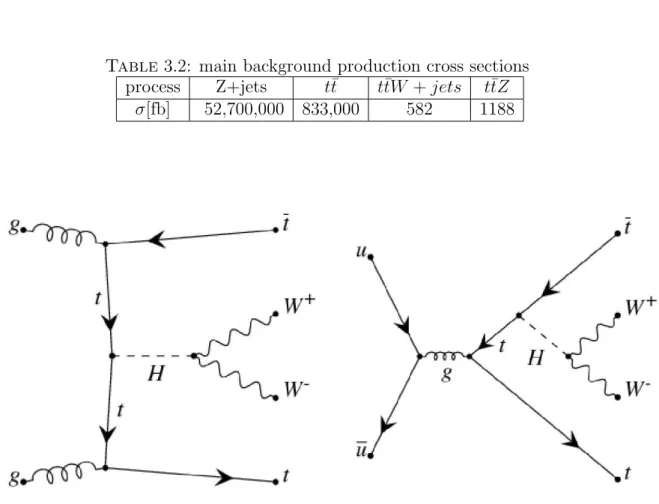
Figure 1.2.5 shows the Feymann diagrams of the four Higgs production mechanisms. The theoretical decay models of Higgs are H → γγ, H → b¯b, H → W W, H → 4leptons, H → t¯t. These channels could be discovery channels at different Higgs mass range. From 100 GeV to 1 TeV, at early integral luminosity. Once Higgs is found, LHC will perform Higgs properties measurements, such as the mass, width, Yukawa Couplings.

t¯_{tH, H → W W}(∗) _{is one of the possible best channels that can measure top quark Yukawa}

Figure 1.3: Higgs production Feyman diagrams at hadron collider

1.2.6

SUSY and Physics beyond Standard Model

Supersymmetry(SUSY) is one of the best extensions of the Standard Model, and SUSY particles hunting is one of the primary physics goals of LHC. SUSY is a theory that introduce the symmetry between bosons and fermions, it predicts that for every particle, there is a particle of same properties except the spin is 1/2 different, which is called its super partner(Nevertheless, SUSY cannot be an exact symmetry since there are no fundamental scalar particles having the same mass as the known fermions). That means for each bosons, there exist a corresponding fermion, and vice-versa. SUSY solves several puzzles compared to Standard Model, such as the calculation of radiative corrections to the SM Higgs boson mass encounters divergences, which are quadratic in the cut-off scale Λ at which the theory stops to be valid and New Physics should appear. It is the so-called hierarchy problem. The Minimal Supersymmetric Standard Model(MSSM) predicts two doublets of Higgs fields, which leads to five Higgs particles. Two CP-even h,H bosons, a

pseudoscalar A boson and two charged H± _{bosons. Of which the lightest Higgs mass is}

less than MZ [6].

Other theories predictions beyond standard model, such as Technicolor theory, can be discovered at LHC. It predicts that the high mass of top quark, partly due to kinematics reason, which could be checked by direct measurement of the Yukawa Coupling between

top quark and Higgs in channel t¯_{tH, H → W W}(∗) _[7].

1.3

Motivations of thesis

1.3.1

Research background

Standard Model has been tested and proved to be correct in the recent decades. While the most important particle -Higgs- that predicted in SM has not yet been found ex-perimentally. Higgs searching and Higgs properties measurements are the physics goals

of recent experiments. LEP experiments performed the precision tests of SM electro-weak parameters(Figure 1.4), and gave the constrains on Higgs mass(Figure 1.5 shows

the constraints on Higgs mass of effective weak mixing angle sin2θlep_{ef f} and MW). All

these constraints come to a upper limit of Higgs mass less than 207 GeV. Meanwhile, the direct searching at LEP gives the Higgs mass lower limit is 114.4 GeV [8]. Further more, due to triviality bound and the vacuum stability bound, Higgs mass constraints

dependent on the new physics energy scale Λc. If Λc ∼TeV, then, Higgs mass should be

in the range of 50GeV ≤ MH ≤ 800GeV . If Λc ∼ ΛGU T, Higgs mass is constrained to

130GeV ≤ MH ≤ 180GeV (figure 1.7). So, a Higgs of intermediate mass is favored.

No Higgs signal has been found in all the experiments until now. The primary goal of LHC is Higgs searching and precision tests of electro-weak theory. It allows Higgs searching from the energy range of ∼100 GeV to 1 TeV(Figure 1.8). LHC will take data in summer of 2008. Once Higgs is discovered at LHC, the properties measurement will became an important goal of experiment. As one of the fundamental properties of Higgs, Yukawa Coupling can give the information of fermions mass origin. In the framework

of Standard Model, from equation 1.19, one can get that gt ≈ 1, It is the biggest one of

fermion Higgs Yukawa Coupling constants. And it is likely to be the first Yukawa Coupling

that could be measured experimentally. Further more, gtis an important parameters that

can distinguish SM Higgs and Multi-Higgs bosons of other model. The TechniColor theory predicts that high top quark mass is partly due to dynamics. Direct measurement of Higgs to Top quark Yukawa Coupling will give important information to distinguish this.

1.3.2

Historical status of the study

As early as 2000, in a Higgs Working Group Summary Report, D. Zeppenfeld et al stud-ied the feasibilities of measuring Higgs Yukawa Couplings at LHC. They proposed the method of combining the results of different Higgs decay channels to measure Higgs to top quark Yukawa Coupling [10, 11, 12, 13, 14]. After that, studies of parton level and

fast simulation were performed, focusing on the feasibility of measuring gt through the

channel of t¯tH [15, 16]. In the work of J. Leveque et al in 2002, based on ATLAS detector

fast simulation(Atlfast), t¯_{tH, H → W W channel is studied in the Higgs mass between 120}

and 200 GeV, and an accuracy of gtthat can reach a maximum of 13% for mH = 160GeV .

However, the fast simulation base on random sampling quantifies is a very crude simula-tion of the ATLAS detector that can not be used for refined analysis. It did not include trigger and pileup effects, and isolation effects are not accurately accounted which

re-sults in the underestimation of t¯t background. Moreover, all these studies did not include

systematics.

The ATLAS full simulation software has recently provide with an accurate

descrip-tion of the real detector behavior. A study of gtmeasurement based on full simulation was

needed before data taking in 2008 with t¯_{tH, H → W W channel. This thesis work based}

on Computing System Commissioning(CSC) full simulation Monte Calor data, fulfill this need. It includes full trigger, pileup and systematics uncertainties studies. However, these studies especially the systematics are relevant to the performance of real detector. The study presented in chapter 5 of 2004 ATLAS detector Combined Test Beam data

pro-Measurement

Fit

|O

meas

O

fit

|/!

meas

0

1

2

3

0

1

2

3

"#

_had

(m

_Z

)

"#

(5)

0.02758 $ 0.00035 0.02767

m

_Z

%GeV&

m

_Z

%GeV&

91.1875 $ 0.0021

91.1875

'

_Z

%GeV&

'

_Z

%GeV&

2.4952 $ 0.0023

2.4958

!

_had

%nb&

!

0

41.540 $ 0.037

41.478

R

_l

R

_l

20.767 $ 0.025

20.743

A

_fb

A

0,l

0.01714 $ 0.00095 0.01644

A

_l

(P

₍

)

A

_l

(P

₍

)

0.1465 $ 0.0032

0.1481

R

_b

R

_b

0.21629 $ 0.00066 0.21582

R

_c

R

_c

0.1721 $ 0.0030

0.1722

A

_fb

A

0,b

0.0992 $ 0.0016

0.1038

A

_fb

A

0,c

0.0707 $ 0.0035

0.0742

A

_b

A

_b

0.923 $ 0.020

0.935

A

_c

A

_c

0.670 $ 0.027

0.668

A

_l

(SLD)

A

_l

(SLD)

0.1513 $ 0.0021

0.1481

sin

2

)

_eff

sin

2

)

lept

(Q

_fb

) 0.2324 $ 0.0012

0.2314

m

_W

%GeV&

m

_W

%GeV&

80.399 $ 0.025

80.376

'

_W

%GeV&

'

_W

%GeV&

2.098 $ 0.048

2.092

m

_t

%GeV&

m

_t

%GeV&

172.4 $ 1.2

172.5

July 2008

Figure 1.4: Summary of electroweak precision measurements at LEP1, LEP2, SLC and the Tevatron; The SM fit results, which have been derived including all radiative correc-tions, and the standard deviations are also shown [9]

Figure 1.5: The measurement [vertical band] and the theoretical prediction [the hatched

bands] for sin2θlep_{ef f} and MW as a function of the Higgs boson mass [9]

vides a unique window to understand the real detector performance with a real detector configuration.

1.3.3

Motivation of the study

Once Higgs is found, the properties measurements of Higgs will become important. gt is

one of Higgs most important properties, which can tell whether it is a SM like Higgs or not.

t¯tH is the best physics channel of gt measurement. According to SM. At the intermediate

Higgs mass range of 120 and 200 GeV, Higgs mainly decays to W W, ZZ, τ τ, γγ, b¯b. And the branching ratio of Higgs decays is dominated by H → W W [17]. So, ttH, H → W W

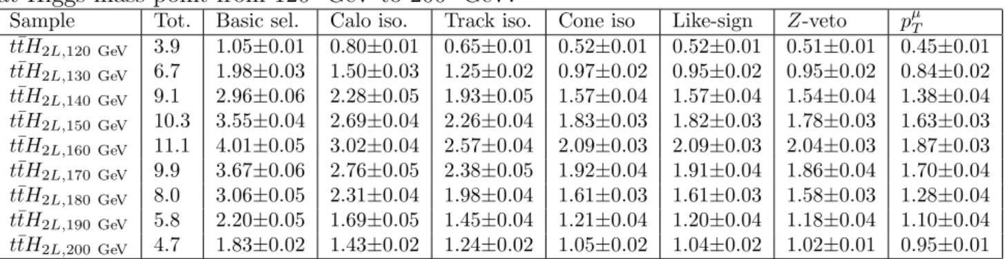
is the most promising channel for gt measurement. In the Higgs mass range of 130 to 200

GeV, ttH, H → W W will gives an accuracy of ∼25% for gtmeasurement(see Chapter 3).

For Higgs mass less than 130 GeV, ttH, H → W W combined with ttH, H → b¯b studies,

give an accurate gt measurement. Furthermore, ttH, H → W W results can be combined

with other channels like H → γγ. It can give the ratios of different Higgs decay model partial width, which are important input for Higgs properties study and new physics searching.

Systematics uncertainties are the dominant error in gt measurement at t¯tH, H →

0

1

2

3

4

5

6

100

30

300

m

_H

GeV!

"

#

2

Excluded

Preliminary

"$

_had

=

"$

(5)

0.02758%0.00035

0.02749%0.00012

incl. low Q

2

data

Theory uncertainty

July 2008 mLimit = 154 GeV

Figure 1.6: The ∆χ2 _{of the fit to the electroweak precision data as a function of M}

H. The

solid line results when all data are included and the blue/shaded band is the estimated theoretical error from unknown higher order corrections. The effect of including the low

Q2 _{data and the use of a different value for ∆α}

Figure 1.7: The triviality (upper) bound and the vacuum stability (lower) bound on the

Higgs boson mass as a function of the New Physics or cut off scale Λc for a top quark

mass mt = 175±6 GeV and αs(MZ) = 0.118±0.002; the allowed region lies between the

bands and the colored/shaded bands illustrate the impact of various uncertainties [3] electron identification efficiency, are important systematics uncertainties sources. The knowledge about the performance of calorimeter, especially the electromagnetic calorime-ter, are essential in this analysis. In the second half of this thesis, analysis of Combined test beam very low energy electron is presented, to understand the energy reconstruction and linearity of electron.

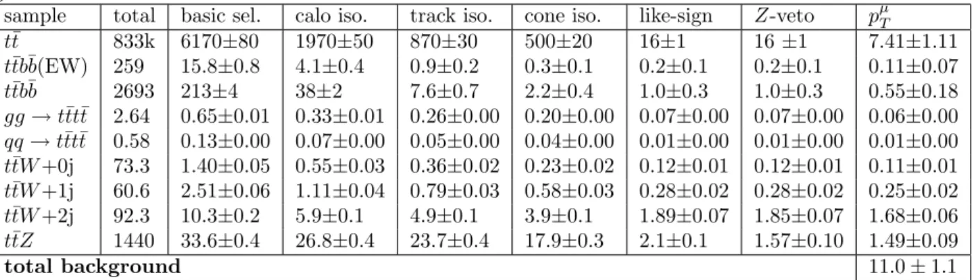
This thesis is the first study using ATLAS full simulation MC data, of the t¯_{tH, H →}

W W(∗) _{with two leptons and three leptons final states. A special Cone isolation is}

pro-posed and developed to suppress background. This analysis on t¯_{tH, H → W W}(∗) _also

includes a detailed studies on systematics uncertainties.

Toward a better understanding of the detector performance and to compare them to full simulation, 2004 ATLAS detector Combined Test Beam data have been analyzed. The chapter 5 present the full analysis of the linearity of VLE electrons using Beam Chamber information and the default calculation. Then, a 5 × 5 multiple seeding clustering method is studied, and given the calibration constants obtained to simulated data. It show that this calibration method may improve the energy linearity in the reconstruction of electrons.

Figure 1.8: ATLAS discovery potential for a Higgs mass range in [100, 1000]GeV [7]

1.3.4

Structure of this thesis

This thesis include the work of my doctoral studies of 2005 to 2008. The contents of each chapter is:

ˆ Chapter one: Introduction of the Higgs searching and gt measurements in particle

physics. Including theoretical motivations and historical status.

ˆ Chapter two: Introduction of Large Hadron Collider and ATLAS detector equip-ments.

ˆ Chapter three: The studies of ttH, H → WW .

ˆ Chapter five: Very Low Energy(VLE) electron linearity studies by using beam cham-ber at single electron level and one possible improvement of the calibration proce-dure.

Introduction of LHC and ATLAS

Contents

2.1 The Large Hardron Collider(LHC) . . . 21 2.2 The ATLAS detector . . . 24 2.2.1 ATLAS detector requirements to fulfill the physics goals . . . . 24 2.2.2 ATLAS designed performance . . . 25 2.2.3 ATLAS overview . . . 26 2.3 Data transportation, storage and analysis of ATLAS . . . 48

2.1

The Large Hardron Collider(LHC)

The Large Hadron Collider(LHC) is an accelerator located at CERN, at the boundaries of France and Switzerland, 20 kilometers from the center of Geneva. The concept of this machine was started in the meddle of the 80s. Before LEP start taking data, scientists already thought of a machine at a high center of mass energy and luminosity that no machine had ever explored, to uncover the structure of mater to a deeper understanding. This project was approved by CERN Council in December 1994 and started its construc-tion from then. Now, this miracle has almost become true and will start running this summer.

The LHC is a proton-proton collider. Its center of mass energy is 14 TeV, hosted in circle tunnel of about 27 km, 100 meters underground(Figure 2.1). In order to keep the 7 TeV proton beam in track, there are about 1232 superconducting dipole magnets in the tunnel. Each of them is 14.2 meters long, and the magnetic field at its maximum is 8.4 tesla [4].

The luminosity of collider can be calculated from:

L = _4π1 N_σ1· N2 · f

x· σy· t

Where N1, N2 are the protons numbers in the two crossing bunches. σx, σy are the transverse sizes of the bunches, f is the fraction of effective bunches, t is the time between

two neighboring collisions. The design luminosity of LHC is 1034 _cm−2_s−1_{. There are}

abundant physics at the energy scale of LHC. Each cross of two bunches will have an average of 23 inelastic interactions of proton to proton. All these reactions in one bunch crossing is defined as one event. Figure 2.2 shows the production cross section of possible physics channels as a function of the center of mass energy at proton-proton collision. Under the center of mass energy of LHC, the total production cross section is about 100mb. Table 2.1 lists the main design parameters of LHC.

LHC parameters value LHC parameters value

Center mass energy 14 TeV Dipole field 8.4 T

Luminosity 1034_cm−2_s−1 _{Beam-Beam parameter 0.0034}

Injection energy 450 GeV circulating current 0.53 A

number of bunchs 2835 Particles per bunch 1.051011

stored energy 334MJ bunch space 25ns

Beam Lifetime 22h Luminorsity Lifetime 10h

Table 2.1: part of LHC important design parameters

The main physics goals of LHC are Higgs searching and precision tests of electro-weak theory. There are four detectors at LHC: ATLAS, CMS, ALICE and LHC-b, of which ATLAS and CMS are general purpose detectors. ALICE is a special purpose detector for heavy ion collision physics. LHC-b is a B physics dedicated detector.

2.2

The ATLAS detector

2.2.1

ATLAS detector requirements to fulfill the physics goals

The ATLAS(A Toroidal ApparatuS) detector is a general purpose detector at LHC. The primary physics goals of this experiment are Higgs searching and electro-weak precision tests, and possible new physics searching. Due to the high luminosity, extreme center of mass energy, and high background over signal ratio at LHC, ATLAS must satisfy the constrains as following:

ˆ Due to the extreme experimental conditions at LHC, ATLAS detector must uses very fast and radiation-hard electronics and sensors. In order to reduce the overlap at high particle fluxes, all sub detectors need fine granularity.

ˆ Large acceptance of pseudorapidity and azimuthal angle coverage are required, to tag and reconstruct physics events of particular interest.

ˆ Good charge particle identification and momentum resolution are required. Mean-while, in order to reconstruct and identify τ lepton and b − jets, good vertexing

ability is needed for vertex detector near the interaction point, to precisely measure the secondary vertexes.

ˆ Good energy measurement and resolution are needed in the electromagnetic calorime-ter, in order to identify photon, electron. And almost full azimuthal coverage of hadron calorimeters is needed, in order to give the precise measurement of missing transverse energy.

ˆ High muon identification efficiency and good muon momentum resolution, of a wide range for both coverage and energy are essential in physics with final states that include muons. Good charge determination even for very high energy muons is also needed.

ˆ Heavy gauge bosons W′ _{and Z}′ _{may be produced at LHC. Considering their leptonic}

decays, ATLAS needs good identification, energy resolution and charge separation power at the level of several TeV.

ˆ In order to reduce the events rates to an acceptable level, and keep as much as pos-sible interesting physics events, a high efficiency trigger system is needed to handle the 40 MHz input to an output of about 200Hz.

2.2.2

ATLAS designed performance

To fulfill the above requirements, the designed ATLAS performance are list in table 2.2:

Detector Component Required Resolution η Coverage

Measurement Trigger Tracking σpT/pT = 0.05%pT ⊕ 1% ±2.5 EM calorimetry σE/E = 10%/ √ E ⊕ 0.7% ±3.2 ±2.5 Hadronic calorimetry

barrel and end-cap σE/E = 50%/

√

E ⊕ 3% ±3.2 ±3.2

forward σE/E = 100%/

√

E ⊕ 10% 3.1 < |η| < 4.9 3.1 < |η| < 4.9

Muon spectrometer σpT/pT = 10% at pT=1TeV ±2.7 ±2.4

Table 2.2: General performance goals of the ATLAS detector. Note that, for high − pT

muons, the muon-spectrometer performance is independent of the inner-detector system. The units for E and pT are in GeV [20].

2.2.3

ATLAS overview

The ATLAS detector is composed of an Inner Detector(ID), a calorimeter system, a muons spectrometer, a trigger and Data Acquisition(DAQ) system. Its dimension are 44 meters long and 25 meters high, for a total of about 7000 tons. The ATLAS detector is located at the IP1(impact point 1) of the tunnel of LHC, about 100 meters underground. Figure 2.4 and 2.3 show the overview of the ATLAS detector and the schematic of its components. The function of the Inner Detector is for vertexing, charge particles tracking and identi-fication. And the Calorimeter system is used for photon, electron, jets identification and energy measurements, the Muon spectrometer is used to track and measure the energy of muons. Magnet system that provides the bending power on charged particles. The coordinate system of ATLAS is defined as following: the beam direction defines the z-axis and the x − y plane is transverse to the beam direction. The positive x − axis is defined as pointing from the interaction point to the center of the LHC ring and the positive y-axis is defined as pointing upwards. The side − A of the detector is corresponding to positive z and side − C to negative z. The azimuthal angle φ is measured around the beam axis, and the polar angle θ is the angle from the beam axis. The pseudorapidity

is defined as η ≡ − ln (tan (θ/2)). The transverse momentum pT , the transverse energy

ET , and the missing transverse energy ET are defined in the x-y plane unless stated otherwise. The distance ∆R in the pseudorapidity-azimuthal angle space is defined as

∆R ≡ p∆η2_{+ ∆φ}2 _{[20]. The following sections will introduce each component of the}

ATLAS detector.

2.2.3.1 Inner Detector

The design goals of ATLAS ID are: Large coverage in azimuthal and pseudorapidity. robust pattern recognizability. Good momentum resolution and secondary vertexing for

charged particles in the acceptance of |η| < 2.5 and above a pT threshold(the threshold

is usually 0.5 GeV, while it is possible to have 0.1 GeV at early stages for some minimal deviation events measurements). Meanwhile, it can provide electron identification of |η| < 2.0 and energy between 0.5 GeV and 150 GeV, even at high luminosity runs of LHC [21] [22]. Its construction reaches the utmost of the modern technics.

ID hosts inside one cylinder of dimension ±3512 mm long, semidiameter of 1150 mm. It is in a solenoid of magnet 2 tesla field (Figure 2.5). The parameters are shown in table 2.3, and the plan view are shown in figure 2.6. Figure 2.7 and figure 2.8 demonstrate a 10 GeV track travels through the barrel and end cap ID sensors separately.

The ID consists of three independent but complementary sub-detectors. At small radii region, there are silicon pixel layers and solid stereo pairs silicon microstrip layers to achieve a robust pattern recognition. At larger radii region, there are Transition Radiation Tracker(TRT), which is composed of multi-layers, up to 73 layers of straws interleaved with fibres (barrel) and 160 straw planes interleaved with foils (end-cap). All charged tracks

with pT > 0.5 GeV and |η| < 2.0 will traverse at least 36 straws of the most regions,

which provide a continuous track and therefore enhance the pattern recognition as well as improve the electron identification performance. Table 2.4 lists the track parameters resolution of each ID sub-detector.

Figure 2.4: Overview of ATLAS detector

Item Radial extension(mm) Length(mm)

Overall ID envelope 0 < R < 1150 _{0 < |z| < 3512}

Beam-pipe 29 < R < 36

Pixel Overall envelope 45.5 < R < 242 _{0 < |z| < 3092}

3 cylindrical layers Sensitive barrel 50.5 < R < 122.5 _{0 < |z| < 400.5}

2 x 3 disks Sensitive end-cap 88.8 < R < 149.6 _{495 < |z| < 650}

SCT Overall envelope 255 < R < 549(barrel) _{0 < |z| < 805}

251 < R < 610(endcap) _{810 < |z| < 2797}

4 cylindrical layers Sensitive barrel 299 < R < 514 _{0 < |z| < 749}

2 x 9 disks Sensitive end-cap 275 < R < 560 _{839 < |z| < 2735}

TRT Overall envelope 554 < R < 1082(barrel) _{0 < |z| < 780}

617 < R < 1106(endcap) _{827 < |z| < 2744}

73 straw planes Sensitive barrel 563 < R < 1066 _{0 < |z| < 712}

160 straw planes Sensitive end-cap 644 < R < 1004 _{848 < |z| < 2710}

Table 2.3: Main parameters of inner detector

Figure 2.6: Plan view of a quarter-section of the ATLAS inner detector showing each of the major detector elements with its active dimensions and envelopes. The labels PP1, PPB1 and PPF1 indicate the patch-panels for the ID services.

Figure 2.7: Drawing showing the sensors and structural elements traversed by a charged

track of 10 GeV pT in the barrel inner detector (η = 0.3). The track traverses successively

the beryllium beam-pipe, the three cylindrical silicon pixel layers with individual sensor

elements of 50 × 400µm2_{, the four cylindrical double layers (one axial and one with}

a stereo angle of 40 mrad) of barrel silicon microstrip sensors (SCT) of pitch 80 µm and approximately 36 axial straws of 4 mm diameter contained in the barrel transition radiation tracker modules within their support structure.

Figure 2.8: Drawing showing the sensors and structural elements traversed by two

charged tracks of 10 GeV pT in the end-cap inner detector (η = 1.4 and 2.2). The

end-cap track at η = 1.4 traverses successively the beryllium beam-pipe, the three

cylin-drical silicon pixel layers with individual sensor elements of 50 × 400µm2_{, four of the}

disks with double layers (one radial and one with a stereo angle of 40 mrad) of end-cap silicon microstrip sensors (SCT) of pitch ∼ 80µm and approximately 40 straws of 4 mm diameter contained in the end-cap transition radiation tracker wheels. In contrast, the end-cap track at η = 2.2 traverses successively the beryllium beam-pipe, only the first of the cylindrical silicon pixel layers, two end-cap pixel disks and the last four disks of the end-cap SCT. The coverage of the end-cap TRT does not extend beyond |η| = 2

Track Parameter _{0.25 < |η| < 0.5 1.50 < |η| < 1.75} σx(∞) pX (GeV) σx(∞) pX (GeV)

Inverse transverse momentum(1/pT) 0.34 T eV−1 44 0.41 T eV−1 80

Azimuthal angle (φ) 70 µ rad 39 92 µ rad 49

Polar angle(cot θ) _{0.7 ×10}−3 5.0 _{1.2 ×10}−3 10

Transverse impact parameter(d0) 10 µ m 14 12 µ m 20

Longitudinal impact parameter(z0× sin θ) 91 µ m 2.3 71 µ m 3.7 Table 2.4: Expected track-parameter resolutions (RMS) at infinite transverse

momen-tum, σx(∞), and transverse momentum, pX, at which the multiple-scattering

contribu-tion equals that from the detector resolucontribu-tion. The momentum and angular resolucontribu-tions are shown for muons, whereas the impact-parameter resolutions are shown for pions. The values are shown for two η-regions, one is in the barrel inner detector where the amount of material is close to its minimum and one is in the end-cap where the amount of material is close to its maximum.

The high radiation environment is a challenge for inner detector sensors, the elec-tronics, and the mechanical structure. Over the life time of 10 years of the designed detector, pixel inner vertexing layer must be replaced after approximately three years of operation at design luminosity. The other pixel layers and the pixel disks must withstand

up to ∼ 8 × 1014_cm−2 _{1MeV neutron equivalent fluency(F}

neq, the equivalent radiation of

1 MeV neutron). While the innermost parts of the SCT must withstand ∼ 2 × 1014_cm−2

Fneq. In order to maintain an adequate noise performance after radiation damage, the

silicon sensors must be kept at low temperature of −5◦_{C ∼ −10}◦_{C by a cooling material}

of −25◦_{C. In contrast, the TRT is designed to operate at room temperature.}

The above operating specifications imply requirements on the alignment precision which are summarized in table 2.5 and which serve as stringent upper limits on the silicon-module build precision, the TRT straw-tube position, and the measured silicon-module placement accuracy and stability.

ˆ Pixel

The pixel modules are 2715 arranged in three barrel layers and two end-caps each with three disk layers. A total of 112 barrel staves and 48 end-cap sectors (8 sectors per disk) form the barrel and disk layers. The minimum pixel module(innermost)

size is 50×400 mm2_{, dictated by the readout pitch of the front-end electronics. There}

are 47232 pixels on each sensor, but for reasons of space there are four ganged pix-els in each column of the front-end chip, thus leading to a total of 46080 readout channels. Each pixel of a sensor is bump-bonded through a hole in the passivation layer to an element of the front-end readout integrated circuit as part of the module. ˆ SCT

SCT consists of 4088 modules tiling four coaxial cylindrical layers in the barrel region and two end-caps each containing nine disk layers. The modules cover a surface of

63m2 _{of silicon and provide almost hermetic coverage with at least four precision}

space-point measurements over the fiducial coverage of the inner detector.

The 2112 barrel SCT modules use 80 µm pitch micro-strip sensors, The sensors are connected to binary signal readout chips. The main parameter of SCT are listed in table 2.6.

ˆ TRT

The TRT contains up to 73 layers of straws interleaved with fibres (barrel) and 160 straw planes interleaved with foils (end-cap), which provide transition radiation for

electron identification. All charged tracks with pT > 0.5GeV, |η| < 2.0 will traverse

at least 36 straws, except in the barrel-end-cap transition region(0.8 < η < 1.0). where this number decreases to a minimum of 22 crossed straws. Typically, seven

Item Intrinsic accuracy Alignment tolerances

(µ m) (µ m)

Radial(R) Axial(z) AZIMUTH(R-φ) Pixel Layer-0 10(R-φ) 115(Z) 10 20 7 Layer-1 and -2 10(R-φ) 115(Z) 20 20 7 Disks 10(R-φ) 115(R) 20 100 7 SCT Barrel 17(R-φ) 580(Z)1 100 50 12 Disks 17(R-φ) 580(R)1 _{50 200 12} TRT 130 302

1. Arises from the 40 mrad stereo angle between back-to-back sensors on the SCT modules with axial (barrel) or radial (end cap) alignment of one side of the structure

The z-resolution results from two axial-stereo points with opposite stereo directions The result is pitch-dependent for end cap SCT modules

2. The quoted alignment accuracy is related to the TRT drift-time accuracy

Table 2.5: Intrinsic measurement accuracies and mechanical alignment tolerances for the inner-detector sub-systems, as defined by the performance requirements of the ATLAS experiment.

to ten high-threshold hits from transition radiation are expected for electrons with energies above 2 GeV.

The barrel TRT is divided into three rings of 32 modules each, supported at each end by a space frame, which is the main component of the barrel support struc-ture. Each module consists of a carbon-fibre laminate shell and an internal array of straws embedded in a matrix of 19 µm-diameter polypropylene fibres serving as the transition radiation material. The straws, form a uniform axial array with a mean spacing of ∼7 mm. The module shells are non projective to reduce the dead region

for high pT tracks

The dimensional specifications are set by the intrinsic straw R − φ resolution of 130 µm. implying that each wire position is constrained to within ±50µm. The module shell, made of 400 µm thick carbon fibre with high thermal conductivity and flat to within 250 µm, is measured to satisfy maximum distortions of < 40µm under full load.

Parameter Description

Strips _{2 × 768 active strips, ± 20 mrad stereo rotation} Nominal resolution 17 µ m in-plane lateral(R-φ)

580 µ m in-plane longitudinal(z or R) Mudule dimensions

-barrel Active length 126.09 mm + 2.09 mm dead space between sensors

-outer end-cap Active length 119.14 mm + 2.09 mm dead space, radius 438.77 - 560.00 mm -middle end-cap Active length 115.61 mm + 2.09 mm dead space, radius 337.60 - 455.30 mm -short-middle end-cap Active length 52.48 mm, radius 402.82 - 455.30 mm

-inner end-cap Active length 59.1 mm, radius 275.00 - 334.10 mm

Specified build Barrel back-to-back in plane: < 8 µ m(lateral) < 20 µ m(longitudinal) tolerance End-cap back-to-back in plane: < 5 µ m(lateral) < 10 µ m(longitudinal)

Barrel out-of-plane(module thickness and sensor bowing): < 70 µ m Barrel envelope: < 200 µ m

End-cap envelope: < 115 µ m

Barrel module fixation points with respect to module center: < 40 µ m End-cap module fixation points with respect to module center: < 20 µ m Build accuracy _{Barrel back-to-back in plane: ± 2.1 µ m(lateral) ± 2.7 µ m(longitudinal)} of accepted _{End-cap back-to-back in plane: ± 1.6 µ m(lateral) ± 1.3 µ m(longitudinal)} modules(RMS) _{Barrel module thickness: ± 33 µ m}

Barrel out-of-plane(sensor bowing): ± 9 µ m End-cap module thickness: ± 15 µ m

End-cap out-of-plane(sensor bowing): ± 20 µ m

Barrel module fixation points with respect to module center ± 10 µ m End-cap module fixation points with respect to module center ± 6 µ m Hybrid power 5.5 - 7.5 W

consumption

Sensor power Up to 460 V bias, < 1W at -7◦_C

consumption

Table 2.6: SCT barrel and end-cap module specifications and the RMS build accuracy for accepted modules. The barrel out-of-plane bowing specifications and the measured results are with respect to an average module shape.

2.2.3.2 Calorimeter system

The ATLAS calorimeters consist of a number of sampling detectors with full φ-symmetry and coverage around the beam axis. The calorimeters closest to the beam-line are housed in three cryostats, one barrel and two end-caps. The barrel cryostat contains the magnetic barrel calorimeter, whereas the two end-cap cryostats each contains an electro-magnetic end-cap calorimeter (EMEC), a hadronic end-cap calorimeter (HEC), located behind the EMEC, and a forward calorimeter (FCal) to cover the region closest to the beam. All these calorimeters use liquid argon as the active detector medium; liquid argon has been chosen for its intrinsic linear behavior, its stability of response over time and its intrinsic radiation-hardness [23] [24].

Figure 2.9: The Cut-away view of ATLAS calorimeter

The precision electromagnetic calorimeters are lead-liquid argon detectors with ac-cordion shape absorbers and electrodes. This geometry allows to have several active layers in depth, three in the precision-measurement region(0 < |η| < 2.5) and two in the 2.5 < |η| < 3.2 region and in the overlap region between the barrel and the EMEC. In the precision-measurement region, an accurate position measurement is obtained by finely segmenting the first compartment in η. The η-direction of photons is determined by the position of the photon cluster in the first and the second compartments. in the region (0 < |η| < 1.8) the electromagnetic calorimeters are complemented by presamplers, an instrumented argon layer, which provides a measurement of the energy lost in front of the electromagnetic calorimeters.

For the outer hadronic calorimeter, the sampling medium consists of scintillator tiles and the absorber medium is steel. The tile calorimeter is composed of three parts,

Barrel End-cap EM calorimeter

Number of layers and |η| coverage

presampler 1 |η| < 1.52 1 1.5 < |η| < 1.8 Calorimeter 3 |η| < 1.35 2 1.375 < |η| < 1.5 2 1.35 < |η| < 1.475 3 1.5 < |η| < 2.5 2 2.5 < |η| < 3.2 Granularity_{∆η × ∆φversus|η|} presampler 0.025 × 0.1 |η| < 1.52 0.025 × 0.1 1.5 < |η| < 1.8 Calorimeter 1st layer 0.025/8 × 0.1 |η| < 1.40 0.050 × 0.1 1.375 < |η| < 1.425 0.025 × 0.025 1.40 < |η| < 1.475 0.025 × 0.1 1.425 < |η| < 1.5 0.025/8 × 0.1 1.5 < |η| < 1.8 0.025/6 × 0.1 1.8 < |η| < 2.0 0.025/4 × 0.1 2.0 < |η| < 2.4 0.025 × 0.1 2.4 < |η| < 2.5 0.1 × 0.1 2.5 < |η| < 3.2 Calorimeter 2nd layer 0.025 × 0.025 |η| < 1.40 0.05 × 0.025 1.375 < |η| < 1.425 0.075 × 0.025 1.40 < |η| < 1.475 0.025 × 0.025 1.425 < |η| < 2.5 0.1 × 0.1 2.5 < |η| < 3.2 Calorimeter 3rd layer 0.05 × 0.025 |η| < 1.35 0.05 × 0.025 1.5 < |η| < 2.5

Number of readout channels

Presampler 7808 1536(both sides)

Calorimeter 101760 62208(both sides)

LAr hadronic end-cap

|η|coverage 1.5 < |η| < 3.2

Number of layers 4

Granularity ∆η × ∆φ 0.1 × 0.1 1.5 < |η| < 2.5

0.2 × 0.2 2.5 < |η| < 3.2

Readout channels 5632(both sides)

LAr forward calorimeter

|η|coverage 3.1 < |η| < 4.9

Number of layers 3

Granularity ∆x × ∆y(cm) F Cal1 : 3.0 × 2.6 3.15 < |η| < 4.30

F Cal1 :∼ 4xfiner 3.10 < |η| < 3.15 4.30 < |η| < 4.83 F Cal2 : 3.3 × 4.2 3.24 < |η| < 4.50 F Cal2 :∼ 4xfiner 3.20 < |η| < 3.24 4.50 < |η| < 4.81 F Cal3 : 3.3 × 4.2 3.32 < |η| < 4.60 F Cal3 :∼ 4xfiner 3.29 < |η| < 3.32 4.60 < |η| < 4.75

Readout channels 3524(both sides)

Scintillator tile calorimeter

Barrel Extended barrel

|η|coverage |η| < 1.0 0.8 < |η| < 1.7

Number of layers 3 3

Granularity ∆η × ∆φ 0.1 × 0.1 0.1 × 0.1

last layer 0.2 × 0.1 0.2 × 0.1

Readout channels 5760 4092(both sides)

Figure 2.10: Cumulative amount of material, in units of interaction length, as a function of |η|, in front of the electromagnetic calorimeters, in the electromagnetic calorimeters themselves, in each hadronic compartment, and the total amount at the end of the active calorimetry. Also shown for completeness is the total amount of material in front of the first active layer of the muon spectrometer (up to |η| < 3.0).

one central barrel and two extended barrels. The choice of this technology provides maximum radial depth for the least cost for ATLAS. The tile calorimeter covers the range of 0 < |η| < 1.7. The hadronic calorimetry is extended to larger pseudorapidity by the HEC, a copper/liquid-argon detector, and the FCal, a copper-tungsten/liquid-argon detector. The hadronic calorimetry thus reaches one of its main design goals, namely coverage 3850 over |η| < 4.9. Figure 2.9 shows the schematic drawing of the calorimeter system. Table 2.7 show the main design parameters of the calorimeter. Figure 2.10 show the mater distribution before and in the calorimeter. The structure of the calorimeter will be introduced in the following section.

ˆ Electromagnetic Calorimeter:

An accordion geometry has been chosen for the absorbers and the electrodes of the barrel and end cap electromagnetic calorimeters. Such a geometry provides naturally a full coverage in φ without any cracks, and a fast extraction of the signal at the rear or at the front of the electrodes. In the barrel, the accordion waves are axial and run in φ, and the folding angles of the waves vary with radius to keep the liquid-argon gap constant. In the end-caps, the waves are parallel to the radial direction and run

axially. Since the liquid-argon gap increases with radius in the end-caps, the wave amplitude and the folding angle of the absorbers and electrodes vary with radius. All these features of the accordion geometry lead to a very uniform performance in terms of linearity and resolution as a function of φ.

Figure 2.11: Sketch of a barrel module where the different layers are clearly visible with the ganging of electrodes in φ . The granularity in η and φ of the cells of each of the three layers and of the trigger towers is also shown.

The barrel electromagnetic calorimeter is made of two half-barrels [25], centered around the z-axis. One half-barrel covers the region with z > 0(0 < η < 1.475) and the other one the region with z < 0(−1.475 < η < 0). The length of each half-barrel is 3.2 m, their inner and outer diameters are 2.8 m and 4 m respectively, and each half-barrel weighs 57 tonnes. One of the module is shown as figure 2.11.

The EMEC calorimeters consist of two wheels, on each side of the electromagnetic barrel. Each wheel is 63 cm thick and weighs 27 tonnes, with external and internal radii at ambient temperature of 2098 mm and 330 mm, respectively. It covers the